The Thirty-Third AAAI Conference on Artificial Intelligence (AAAI-19)
Large-Scale Interactive
Recommendation with Tree-Structured Policy Gradient
Haokun Chen,
1Xinyi Dai,
1Han Cai,
1Weinan Zhang,
1Xuejian Wang,
1Ruiming Tang,
2Yuzhou Zhang,
2Yong Yu
11Shanghai Jiao Tong University
2Huawei Noah’s Ark Lab
{chenhaokun,xydai,hcai,wnzhang,xjwang,yyu}@apex.sjtu.edu.cn {tangruiming,zhangyuzhou3}@huawei.com
Abstract
Reinforcement learning (RL) has recently been introduced to interactive recommender systems (IRS) because of its nature of learning from dynamic interactions and planning for long-run performance. As IRS is always with thousands of items to recommend (i.e., thousands of actions), most existing RL-based methods, however, fail to handle such a large discrete action space problem and thus become inefficient. The ex-isting work that tries to deal with the large discrete action space problem by utilizing the deep deterministic policy gra-dient framework suffers from the inconsistency between the continuous action representation (the output of the actor net-work) and the real discrete action. To avoid such inconsis-tency and achieve high efficiency and recommendation ef-fectiveness, in this paper, we propose a Tree-structured Pol-icy Gradient Recommendation (TPGR) framework, where a balanced hierarchical clustering tree is built over the items and picking an item is formulated as seeking a path from the root to a certain leaf of the tree. Extensive experiments on carefully-designed environments based on two real-world datasets demonstrate that our model provides superior recom-mendation performance and significant efficiency improve-ment over state-of-the-art methods.
Introduction
Interactive recommender systems (IRS) (Zhao, Zhang, and Wang 2013) play a key role in most personalized services, such as Pandora, Musical.ly and YouTube, etc. Different from the conventional recommendation settings (Mooney and Roy 2000; Koren, Bell, and Volinsky 2009), where the recommendation process is regarded as a static one, an IRS consecutively recommends items to individual users and re-ceives their feedbacks which makes it possible to refine its recommendation policy during such interactive processes.
To handle the interactive nature, some efforts have been made by modeling the recommendation process as a multi-armed bandit (MAB) problem (Li et al. 2010; Zhao, Zhang, and Wang 2013). However, these works pre-assume that the underlying user preference remains unchanged during the recommendation process (Zhao, Zhang, and Wang 2013) and do not plan for long-run performance explicitly.
Recently, reinforcement learning (RL) (Sutton and Barto 1998), which has achieved remarkable success in various
Copyright c2019, Association for the Advancement of Artificial Intelligence (www.aaai.org). All rights reserved.
challenging scenarios that require both dynamic interac-tion and long-run planning such as playing games (Mnih et al. 2015; Silver et al. 2016) and regulating ad bidding (Cai et al. 2017; Jin et al. 2018), has been introduced to model the recommendation process and shows its potential to handle the interactive nature in IRS (Zheng et al. 2018; Zhao et al. 2018b; 2018a).
However, most existing RL techniques cannot handle the large discrete action space problem in IRS as the time com-plexity of making a decision is linear to the size of the ac-tion space. Specifically, all Deep Q-Network (DQN) based methods (Zheng et al. 2018; Zhao et al. 2018b) involve a maximization operation taken over the action space to make a decision, which becomes intractable when the size of the action space, i.e., the number of available items, is large (Dulac-Arnold et al. 2015), which is very common in IRS. Most Deep Deterministic Policy Gradient (DDPG) based methods (Zhao et al. 2018a; Hu et al. 2018) also suffer from the same problem as a specific ranking function is applied over all items to pick the one with highest score when mak-ing a decision. To reduce the time complexity, Dulac-Arnold et al. (2015) propose to select the proto-action in a continu-ous hidden space and then pick the valid item via a nearest-neighbor method. However, such a method suffers from the inconsistency between the learned continuous action and the actually desired discrete action, and thereby may lead to un-satisfied results (Tavakoli, Pardo, and Kormushev 2018).
In this paper, we propose a Tree-structured Policy Gra-dient Recommendation (TPGR) framework which achieves high efficiency and high effectiveness at the same time. In the TPGR framework, a balanced hierarchical clustering tree is built over the items and picking an item is thus formulated as seeking a path from the root to a certain leaf of the tree, which dramatically reduces the time complexity in both the training and the decision making stages. We utilize policy gradient technique (Sutton et al. 2000) to learn how to make recommendation decisions so as to maximize long-run re-wards. To the best of our knowledge, this is the first work of building tree-structured stochastic policy for large-scale interactive recommendation.
real-world datasets with different settings show superior per-formance and significant efficiency improvement of the pro-posed TPGR over state-of-the-art methods.
Related Work and Background
Advanced Recommendation Algorithms for IRS
MAB-based Recommendation A group of works (Li et al. 2010; Chapelle and Li 2011; Zhao, Zhang, and Wang 2013; Zeng et al. 2016; Wang, Wu, and Wang 2016) try to model the interactive recommendation as a MAB prob-lem. Li et al. (2010) adopt a linear model to estimate the Upper Confidence Bound (UCB) for each arm. Chapelle and Li (2011) utilize the Thompson sampling technique to address the trade-off between exploration and exploitation. Besides, some researchers try to combine MAB with ma-trix factorization technique (Zhao, Zhang, and Wang 2013; Kawale et al. 2015; Wang, Wu, and Wang 2017).
RL-based Recommendation RL-based recommendation methods (Tan, Lu, and Li 2017; Zheng et al. 2018; Zhao et al. 2018b; 2018a), which formulate the recommendation procedure as a Markov Decision Process (MDP), explicitly model the dynamic user status and plan for long-run perfor-mance. Zhao et al. (2018b) incorporate negative as well as positive feedbacks into a DQN framework (Mnih et al. 2015) and propose to maximize the difference of Q-values between the target and the competitor items. Zheng et al. (2018) com-bine DQN and Dueling Bandit Gradient Decent (DBGD) (Grotov and de Rijke 2016) to conduct online news recom-mendation. Zhao et al. (2018a) propose to utilize a DDPG framework (Lillicrap et al. 2015) with a page-display ap-proach for page-wise recommendation.
Large Discrete Action Space Problem in RL-based
Recommendation
Most RL-based models become unacceptably inefficient for IRS with large discrete action space as the time complexity of making a decision is linear to the size of the action space. For all DQN-based solutions (Zhao et al. 2018b; Zheng et al. 2018), a value functionQ(s, a), which estimates the ex-pected discounted cumulative reward when taking the action aat the states, is learned and the policy’s decision is:
πQ(s) = argmax
a∈A
Q(s, a). (1)
As shown in Eq. (1), to make a decision,|A|(Adenotes the item set) evaluations are required, which makes both learning and utilization intractable for tasks where the size of the action space is large, which is common for IRS.
Similar problem exists in most DDPG-based solutions (Zhao et al. 2018a; Hu et al. 2018) where some ranking pa-rameters are learned and a specific ranking function is ap-plied over all items to pick the one with highest ranking score. Thus, the complexity of sampling an action for these methods also grows linearly with respect to|A|.
Dulac-Arnold et al. (2015) attempt to address the large discrete action space problem based on the DDPG frame-work by mapping each discrete action to a low-dimensional continuous vector in a hidden space while maintaining an
actor network to generate a continuous vectoravin the
hid-den space which is later mapped to a specific valid action aamong thek-nearest neighbors ofav. Meanwhile, a value
networkQ(s, a)is learned using transitions collected by ex-ecuting the valid actionaand the actor network is updated according to ∂Q∂(s,ˆaaˆ)aˆ=a
v following the DDPG framework.
Though such a method can reduce the time complexity of making a decision from O(|A|) toO(log(|A|))when the value ofk(i.e., the number of nearest neighbors to find) is small, there is no guarantee that the actor network is learned in a correct direction as in the original DDPG. The reason is that the value networkQ(s, a)may behave differently on the output of the actor network av (when training the
ac-tor network) and the actually executed actiona(when train-ing the value network). Besides, the utilized approximate k-nearest neighbors (KNN) method may also cause trouble as the found neighbors may not be exactly the nearest ones.
In this paper, we propose a novel solution to address the large discrete action space problem. Instead of using the continuous hidden space, we build a balanced tree to rep-resent the discrete action space where each leaf node corre-sponds to an action and top-down decisions are made from the root to a specific leaf node to take an action, which re-duces the time complexity of making a decision fromO(|A|)
toO(d×|A|1/d), whereddenotes the depth of the tree. Since
such a method does not involve a mapping from the continu-ous space to the discrete space, it avoids the gap between the continuous vector given by the actor network and the actu-ally executed discrete action in (Dulac-Arnold et al. 2015), which could lead to incorrect updates.
Proposed Model
Problem Definition
We use an MDP to model the recommendation process, where the key components are defined as follows.
• State. A state sis defined as the historical interactions between a user and the recommender system, which can be encoded as a low-dimensional vector via a recurrent neural network (RNN) (see Figure 2).
• Action.An actionais to pick an item for recommenda-tion, such as a song or a video, etc.
• Reward.In our formulation, all users interacting with the recommender system form the environment that returns a rewardrafter receiving an actionaat the states, which reflects the user’s feedback to the recommended item. • Transition.As the state is the historical interactions, once
a new item is recommended and the corresponding user’s feedback is given, the state transition is determined. An episode in the above defined MDP corresponds to one recommendation process, which is a sequence of user states, recommendation actions and user’s feedbacks, e.g.,
(s1, a1, r1, s2, a2, r2,· · · , sn, an, rn, sn+1). In this case,
the sequence starts with user state s1 and then transits to
s2 after a recommendation action a1 is carried out by the
recommender system and a reward r1 is given by the
sn+1when some pre-defined conditions are satisfied.
With-out loss of generality, we set the length of an episodento a fixed number (Cai et al. 2017; Zhao et al. 2018b).
Tree-structured Policy Gradient Recommendation
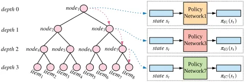
Intuition for TPGR To handle the large discrete action space problem and achieve high recommendation effective-ness, we propose to build up a balanced hierarchical cluster-ing tree over items (Figure 1 left) and then utilize the policy gradient technique to learn the strategy of choosing the op-timal subclass at each non-leaf node of the constructed tree (Figure 1 right). Specifically, in the clustering tree, each leaf node is mapped to a certain item (Figure 1 left) and each non-leaf node is associated with a policy network (note that only three but not all policy networks are shown in the right part of Figure 1 for the ease of presentation). As such, given a state and guided by the policy networks, a top-down mov-ing is performed from the root to a leaf node and the corre-sponding item is recommended to the user.
Balanced Hierarchical Clustering over Items Hierar-chical clustering seeks to build a hierarchy of clusters, i.e., a clustering tree. One popular method is the divisive approach where the original data points are divided into several clus-ters, and each cluster is further divided into smaller sub-clusters. The division is repeated until each sub-cluster is associated with only one point.
In this paper, we aim to conduct balanced hierarchical clustering over items, where the constructed clustering tree is supposed to be balanced, i.e., for each node, the heights of its subtrees differ by at most one and the subtrees are also balanced. For the ease of presentation and implementation, it is also required that each non-leaf node has the same num-ber of child nodes, denoted asc, except for parents of leaf nodes, whose numbers of child nodes are at mostc.
We can perform balanced hierarchical clustering over items following a clustering algorithm which takes a group of vectors and an integercas input and divides the vectors intocbalanced clusters (i.e., the item number of each clus-ter differs from each other by at most one). In this paper, we consider two kinds of clustering algorithms, i.e., PCA-based and K-means-PCA-based clustering algorithms whose de-tailed procedures are provided in the appendices. By repeat-edly applying the clustering algorithm until each sub-cluster is associated with only one item, a balanced clustering tree is constructed. As such, denoting the item set and the depth of the balanced clustering tree asAanddrespectively, we have:
cd−1<|A| ≤cd. (2) Thus, givenA andd, we can setc = ceil(|A|d1)where
ceil(x)returns the smallest integer which is no less thanx. The balanced hierarchical clustering over items is nor-mally performed on the (vector) representation of the items, which may largely affect the quality of the attained balanced clustering tree. In this work we consider three approaches for producing such representation:
• Rating-based.An item is represented as the correspond-ing column of the user-item ratcorrespond-ing matrix, where the value of each element(i, j)is the rating of userito itemj.
Figure 1: Architecture of TPGR.
• VAE-based.Low-dimensional representation of the rat-ing vector for each item can be learned by utilizrat-ing a vari-ational auto-encoder (VAE) (Kingma and Welling 2013). • MF-based.The matrix factorization (MF) technique
(Ko-ren, Bell, and Volinsky 2009) can also be utilized to learn a representation vector for each item.
Architecture of TPGR The architecture of the Tree-structured Policy Gradient Recommendation (TPGR) is based on the constructed clustering tree. To ease the illustra-tion, we assume that there is a status point to indicate which node is currently located. Thus, picking an item is to move the status point from the root to a certain leaf. Each non-leaf node of the tree is associated with a policy network which is implemented as a fully-connected neural network with a softmax activation function on the output layer. Considering nodevwhere the status point is located, the policy network associated withvtakes the current state as input and outputs a probability distribution over all child nodes of v, which indicates the probability of moving to each child node ofv.
Using a recommendation scenario with 8 items for illus-tration, the constructed balanced clustering tree with the tree depth set to 3 is shown in Figure 1 (left). For a given state st, the status point is initially located at the root (node1)
and moves to one of its child nodes (node3) according to
the probability distribution given by the policy network cor-responding to the root (node1). And the status point keeps
moving until reaching a leaf node and the corresponding item (item8in Figure 1) is recommended to the user.
We use the REINFORCE algorithm (Williams 1992) to train the model while other policy gradient algorithms can be utilized analogously. The objective is to maximize the expected discounted cumulative rewards, i.e.,
J(πθ) =Eπθ hXn
i=1
γi−1ri i
, (3)
and one of its approximate gradient with respect to the pa-rameters is:
∇θJ(πθ)≈Eπθ[∇θlogπθ(a|s)Q
πθ(s, a)], (4)
where πθ(a|s)is the probability of taking the action a at
the states, andQπθ(s, a)denotes the expected discounted
cumulative rewards starting withsanda, which can be es-timated empirically by sampling trajectories following the policyπθ.
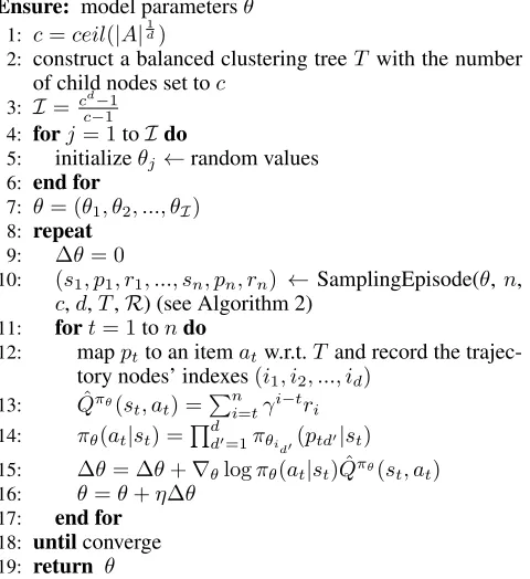
Algorithm 1Learning TPGR
Require: episode lengthn, tree depthd, discount factorγ, learning rateη, reward functionR, item setAwith rep-resentation vectors
Ensure: model parametersθ
1: c=ceil(|A|1d)
2: construct a balanced clustering treeT with the number of child nodes set toc
3: I =ccd−−11
4: forj= 1toIdo
5: initializeθj ←random values 6: end for
7: θ= (θ1, θ2, ..., θI) 8: repeat
9: ∆θ= 0
10: (s1, p1, r1, ..., sn, pn, rn) ←SamplingEpisode(θ,n,
c,d,T,R) (see Algorithm 2)
11: fort= 1tondo
12: mapptto an itematw.r.t.T and record the
trajec-tory nodes’ indexes(i1, i2, ..., id) 13: Qˆπθ(s
t, at) =P n
i=tγi−tri 14: πθ(at|st) =Q
d
d0=1πθid0(ptd0|st)
15: ∆θ= ∆θ+∇θlogπθ(at|st) ˆQπθ(st, at)
16: θ=θ+η∆θ
17: end for
18: untilconverge
19: return θ
(as shown in Algorithm 2),ptdenotes the path from the root
to a leaf at timestept, which consists ofdchoices, and each choice is represented as an integer between1andcdenoting the corresponding child node to move. Making the consec-utive choices corresponding toptfrom the root, we traverse
the nodes alongptand finally reach a leaf node. As such, a
pathptis mapped to a recommended itemat, thus the
prob-ability of choosing at given statest is the product of the
probability of making each choice (to reachat) alongpt.
Time and Space Complexity Analysis Empirically, the value of the tree depthdis set to a small constant (typically set to 2 in our experiments). Thus, both the time (for making a decision) and the space complexity of each policy network isO(c)(see more details in the appendices).
Considering the time spent on sampling an action given a specific state in Algorithm 2, the TPGR makesdchoices, each of which is based on a policy network with at mostc output units. Therefore, the time complexity of sampling one item in the TPGR isO(d×c)' O(d× |A|d1). Compared
to the normal RL-based methods whose time complexity of sampling an action isO(|A|), our proposed TPGR can sig-nificantly reduce the time complexity.
The space complexity of each policy network isO(c)and the number of non-leaf nodes (i.e., the number of policy net-works) of the constructed clustering tree is:
I= 1 +c+c2+· · ·+cd−1= c
d−1
c−1 . (5)
Algorithm 2Sampling Episode for TPGR
Require: parametersθ, episode lengthn, maximum child numberc, tree depthd, balanced clustering treeT, re-ward functionR
Ensure: an episodeE
1: Initializes1←[0]
2: fort= 1tondo
3: node index= 1
4: ford0= 1toddo
5: samplecd0 ∼πθ
node index(st)
6: node index= (node index−1)×c+cd0+ 1
7: end for
8: pt= (c1, c2, ..., cd)
9: mapptto an itematw.r.t.T 10: rt=R(st, at)
11: ift < nthen
12: calculatest+1as described in Figure 2
13: end if
14: end for
15: return E= (s1, p1, r1, ..., sn, pn, rn)
Therefore, the space complexity of the TPGR isO(I × c)' O(ccd−−11×c) ' O(cd) ' O(|A|), which is the same
as that of normal RL-based methods.
State Representation
In this section, we present the state representation scheme adopted in this work, whose details are shown in Figure 2.
Figure 2: State representation.
In Figure 2, we assume that the recommender system is performing the t-th recommendation. The input is a se-quence of recommended item IDs and the corresponding re-wards (user’s feedbacks) before timestept. Each item ID is mapped to an embedding vector which can be learned to-gether with the policy networks in an end-to-end manner, or can be pre-trained by some supervised learning models such as matrix factorization and is fixed while training. Each re-ward is mapped to a one-hot vector with a simple rere-ward mapping function (see more details in the appendices).
For encoding the historical interactions, we adopt a sim-ple recurrent unit (SRU) (Lei and Zhang 2017), an RNN model that is fast to train, to learn the hidden representation. Besides, to further integrate more feedback information, we construct a vector, denoted asuser statust−1 in Figure 2,
concate-nated with the hidden vector generated by the SRU to gain the state representation at timestept.
Experiments and Results
Datasets
We adopt the following two datasets in our experiments. • MovieLens (10M).1A dataset consists of 10 million
rat-ings from users to movies in MovieLens website. • Netflix.2A dataset contains 100 million ratings from
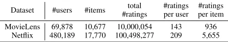
Net-flix’s competition to improve their recommender systems. Detailed statistic information, including the number of users, items and ratings, of these datasets is given in Table 1.
Table 1: Statistic information of the datasets.
Dataset #users #items #ratingstotal #ratingsper user #ratingsper item
MovieLens 69,878 10,677 10,000,054 143 936
Netflix 480,189 17,770 100,498,277 209 5,655
Data Analysis
To demonstrate the existence of hidden sequential patterns in the recommendation process, we empirically analyze the aforementioned two datasets where each rating is attached with a timestamp. Each dataset comprises numerous user sessions and each session contains the ratings from one spe-cific user to various items along timestamps.
Without loss of generality, we regard the ratings higher than 3 as positive ratings (noticed that the highest rating is 5) and the others as negative ratings. For a rating with at most bconsecutive positive (negative) ratings before it, we define its consecutive positive (negative) count asb. As such, each rating can be associated with a specific consecutive positive (negative) count and we can calculate the average rating for ratings with the same consecutive positive (negative) count. We present the corresponding average ratings w.r.t. the consecutive positive (negative) counts in Figure 3, where we can clearly observe the sequential patterns in the user’s rat-ing behavior: a user tends to give a linearly higher ratrat-ing for an item with larger consecutive positive count (green line) and vice versa (red line). The reason may be that the more satisfying (disappointing) items a user has consumed before, the more pleasure (displeasure) she gains and as a result, she tends to give a higher (lower) rating to the current item.
Environment Simulator and Reward Function
To train and test RL-based recommendation algorithms, a straightforward way is to conduct online experiments where the recommender system can directly interact with real users, which, however, could be too expensive and commer-cially risky for the platform (Zhang, Paquet, and Hofmann 2016). Thus, in this paper, we focus on evaluating our pro-posed model on public available offline datasets by building up an environment simulator to mimic online environments.
1
http://files.grouplens.org/datasets/movielens/ml-10m.zip 2
https://www.kaggle.com/netflix-inc/netflix-prize-data
1 2 3 4 5
consecutive count 3.0
3.2 3.4 3.6 3.8 4.0
average rating
MovieLens positive
negative overall
1 2 3 4 5
consecutive count 3.3
3.4 3.5 3.6 3.7 3.8
average rating
Netflix positive negative overall
Figure 3: Average ratings for different consecutive counts.
Specifically, we normalize the ratings of a dataset into range [−1,1]and use the normalized value as the empiri-cal reward of the corresponding recommendation. To take the sequential patterns into account, we combine a sequen-tial reward with the empirical reward to construct the final reward function. Within each episode, the environment sim-ulator randomly samples a useriand the recommender sys-tem starts to interact with the sampled useriuntil the end of the episode, and the reward of recommending itemjto user i, denoted as actiona, at statesis given as:
R(s, a) =rij+α×(cp−cn), (6)
whererij is the corresponding normalized rating and is set
to0if useridoes not rate itemj in the dataset,cp andcn
denote the consecutive positive and negative counts respec-tively;αis a non-negative parameter to control the trade-off between the empirical reward and the sequential reward.
Main Experiments
Compared Methods We compare our TPGR model with 7 methods in our experiments where Popularity and GreedySVD are conventional recommendation methods; LinearUCB and HLinearUCB are MAB-based methods; DDPG-KNN, DDPG-R and DQN-R are RL-based methods. • Popularityrecommends the most popular item (i.e., the item with highest average rating) from current available items to the user at each timestep.
• GreedySVD trains the singular value decomposition (SVD) model after each interaction and picks the item with highest rating predicted by the SVD model.
• LinearUCBis a contextual-bandit recommendation ap-proach (Li et al. 2010) which adopts a linear model to es-timate the upper confidence bound (UCB) for each arm. • HLinearUCB is also a contextual-bandit
recommenda-tion approach (Wang, Wu, and Wang 2016) which learns extra hidden features for each arm to model the reward. • DDPG-KNN denotes the method (Dulac-Arnold et al.
2015) addressing the large discrete action space problem by combining DDPG with an approximate KNN method. • DDPG-R denotes the DDPG-based recommendation method (Zhao et al. 2018a) which learns a ranking vec-tor and picks the item with highest ranking score. • DQN-R denotes the DQN-based recommendation
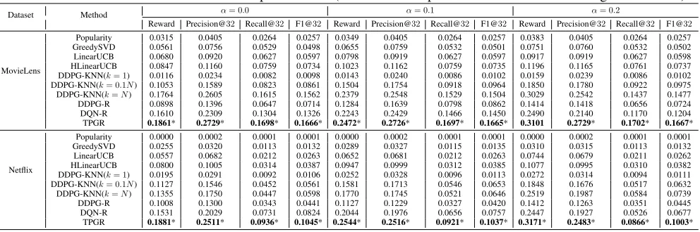
Table 2: Overall interactive recommendation performance (* indicates that p-value is less than10−6for significance test).
Dataset Method α= 0.0 α= 0.1 α= 0.2
Reward Precision@32 Recall@32 F1@32 Reward Precision@32 Recall@32 F1@32 Reward Precision@32 Recall@32 F1@32
MovieLens
Popularity 0.0315 0.0405 0.0264 0.0257 0.0349 0.0405 0.0264 0.0257 0.0383 0.0405 0.0264 0.0257 GreedySVD 0.0561 0.0756 0.0529 0.0498 0.0655 0.0759 0.0532 0.0501 0.0751 0.0760 0.0532 0.0502 LinearUCB 0.0680 0.0920 0.0627 0.0597 0.0798 0.0919 0.0627 0.0597 0.0917 0.0919 0.0627 0.0598 HLinearUCB 0.0847 0.1160 0.0759 0.0734 0.1023 0.1162 0.0759 0.0735 0.1196 0.1165 0.0761 0.0737 DDPG-KNN(k= 1) 0.0116 0.0234 0.0082 0.0098 0.0143 0.0240 0.0086 0.0102 0.0159 0.0239 0.0086 0.0102 DDPG-KNN(k= 0.1N) 0.1053 0.1589 0.0823 0.0861 0.1504 0.1754 0.0918 0.0964 0.1850 0.1780 0.0922 0.0975 DDPG-KNN(k=N) 0.1764 0.2605 0.1615 0.1562 0.2379 0.2548 0.1529 0.1504 0.3029 0.2542 0.1437 0.1477 DDPG-R 0.0898 0.1396 0.0647 0.0714 0.1284 0.1639 0.0798 0.0862 0.1414 0.1418 0.0656 0.0724 DQN-R 0.1610 0.2309 0.1304 0.1326 0.2243 0.2429 0.1466 0.1450 0.2490 0.2140 0.1170 0.1204 TPGR 0.1861* 0.2729* 0.1698* 0.1666* 0.2472* 0.2726* 0.1697* 0.1665* 0.3101 0.2729* 0.1702* 0.1667*
Netflix
Popularity 0.0000 0.0002 0.0001 0.0001 0.0000 0.0002 0.0001 0.0001 0.0000 0.0002 0.0001 0.0001 GreedySVD 0.0255 0.0320 0.0113 0.0132 0.0289 0.0327 0.0115 0.0135 0.0310 0.0315 0.0113 0.0132 LinearUCB 0.0557 0.0682 0.0212 0.0263 0.0652 0.0681 0.0212 0.0263 0.0744 0.0679 0.0211 0.0262 HLinearUCB 0.0800 0.1005 0.0314 0.0387 0.0947 0.0999 0.0312 0.0385 0.1077 0.0995 0.0310 0.0382 DDPG-KNN(k= 1) 0.0195 0.0291 0.0092 0.0106 0.0252 0.0328 0.0096 0.0113 0.0272 0.0314 0.0094 0.0111 DDPG-KNN(k= 0.1N) 0.1127 0.1546 0.0452 0.0561 0.1581 0.1713 0.0546 0.0653 0.1848 0.1676 0.0517 0.0632 DDPG-KNN(k=N) 0.1355 0.1750 0.0447 0.0598 0.1770 0.1745 0.0521 0.0646 0.2519 0.1987 0.0584 0.0739 DDPG-R 0.1008 0.1300 0.0343 0.0441 0.1127 0.1229 0.0327 0.0420 0.1412 0.1263 0.0351 0.0445 DQN-R 0.1531 0.2029 0.0731 0.0824 0.2044 0.1976 0.0656 0.0757 0.2447 0.1927 0.0526 0.0677 TPGR 0.1881* 0.2511* 0.0936* 0.1045* 0.2544* 0.2516* 0.0921* 0.1037* 0.3171* 0.2483* 0.0866* 0.1003*
Experiment Details For each dataset, the users are ran-domly divided into two parts where 80% of the users are used for training while the other 20% are used for test. In our experiments, the length of an episode is set to 32 and the trade-off factorαin the reward function is set to0.0,0.1and
0.2respectively for both datasets. In each episode, once an item is recommended, it is removed from the set of available items, thus no repeated items occur in an episode.
For DDPG-KNN, larger k (i.e., the number of nearest neighbors) leads to better performance but poorer efficiency and vice versa (Dulac-Arnold et al. 2015). For fair compar-ison, we consider three cases with the value ofk set to 1, 0.1NandN (Ndenotes the number of items) respectively.
For TPGR, we set the clustering tree depthdto 2 and ap-ply the PCA-based clustering algorithm with rating-based item representation when constructing the balanced tree since they give the best empirical results as shown in the following section. The implementation code3 of the TPGR is available online.
All other hyper-parameters of all the models are carefully chosen by grid search.
Evaluation Metrics As the target of RL-based methods is to gain the optimal long-run rewards, we use the average re-ward over each recommendation for each user in test set as one evaluation metric. Furthermore, we adopt Precision@k, Recall@kand F1@k(Herlocker et al. 2004) as our evalua-tion metrics. Specifically, we set the value ofkas 32, which is the same as the episode length. For each user, all the items with a rating higher than 3.0 are regarded as the relevant items while the others are regarded as the irrelevant ones.
Results and Analysis In our experiments, all the mod-els are evaluated in term of the four metrics including av-erage reward over each recommendation, Precision@32, Recall@32, and F1@32. The summarized results are pre-sented in Table 2 with respect to the two datasets and three different settings of trade-off factorαin the reward function. From Table 2, we observe that our proposed TPGR out-performs all the compared methods in all settings with
p-3
https://github.com/chenhaokun/TPGR
values less than10−6(indicated by a * mark in Table 2) for
significance test (Ruxton 2006) in most cases, which demon-strates the performance superiority of the TPGR.
When comparing the RL-based methods with the con-ventional and the MAB-based methods, it is not surpris-ing to find that the RL-based models provide superior per-formances in most cases, as they have the ability of long-run planning and dynamic adaptation which is lacking in other methods. Among all the RL-based methods, our pro-posed TPGR achieves the best performance, which can be explained by two reasons. First, the hierarchical clustering over items incorporates additional item similarity informa-tion into our model, e.g., similar items tend to be clus-tered into one subtree of the clustering tree. Second, differ-ent from normal RL-based methods which utilize one com-plicated neural network to make decisions, we propose to conduct a tree-structured decomposition and adopt a certain number of policy networks with much simpler architectures, which may ease the training process and lead to better per-formance.
Besides, as the value of trade-off factorαincreases, we observe that the improvement of TPGR over HLinearUCB (i.e., the best non-RL-based method in our experiments) in terms of average reward becomes more significant, which demonstrates that the TPGR do have the capacity of captur-ing sequential patterns to maximize long-run rewards.
Table 3: Time comparison for training and decision making.
Method Seconds per training step Seconds per10
6decisions
MovieLens Netflix MovieLens Netflix
DQN-R 13.1 15.3 19.6 34.6
DDPG-R 44.6 58.6 29.4 49.6
DDPG-KNN(k= 1) 1.3 1.3 1.8 1.8 DDPG-KNN(k= 0.1N) 24.2 40.3 200.4 313.0
DDPG-KNN(k=N) 248.4 323.9 1,875.0 3,073.2
TPGR 3.0 3.1 3.4 3.9
the model with those episodes) and the consumed time for making 1 million decisions for each model.
As shown in Table 3, TPGR consumes much less time for both the training and the decision making stages compared to DQN-R and DDPG-R. DDPG-KNN withkset to 1 gains high efficiency, which, however, is meaningless because it achieves very poor recommendation performance as shown in Table 2. In another case where k is set to N, DDPG-KNN suffers from high time complexity which makes it even much slower than DQN-R and R. Thus, DDPG-KNN can not achieve high effectiveness and high efficiency at the same time. Compared to the case that DDPG-KNN makes a trade-off between effectiveness and efficiency, i.e., settingkas0.1N, our proposed TPGR achieves significant improvement in term of both effectiveness and efficiency.
Influence of Clustering Approach
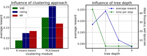
Since the architecture of the TPGR is based on the bal-anced hierarchical clustering tree, it is essential to choose a suitable clustering approach. In the previous section, we in-troduce two clustering modules, K-means-based and PCA-based modules, and three methods to represent an item, namely rating-based, MF-based and VAE-based methods. As such, there are six combinations to conduct balanced hierarchical clustering. Withαset to 0.1, we evaluate the above six approaches in term of average reward on Netflix dataset. The results are shown in Figure 4 (left).
K-means-based PCA-based
clustering module
0.05 0.10 0.15 0.20 0.25
average reward
Influence of clustering approach VAE
rating MF
1 2 3 4
tree depth
0.240 0.245 0.250 0.255
average reward
10 20 30 40
seconds per training step
Influence of tree depth average reward time per step
Figure 4: Influence of clustering approach and tree depth.
As shown in Figure 4 (left), applying PCA-based cluster-ing module with ratcluster-ing-based item representation achieves the best performance. Two reasons may account for this re-sult. First, the rating-based representation retains all the in-teraction information between the users and the items, while both the VAE-based and the MF-based representations are low-dimensional, which retain less information than rating-based representation after dimension reduction. Therefore, using rating-based representation may lead to better cluster-ing. Second, as the number of clustersc (i.e., child nodes
number of non-leaf nodes) is large (134 for Netflix dataset with the tree depth set to 2), the quality of the clustering tree derived from K-means-based method would be sensitive to the choices of the initialization of center points and the dis-tance function, etc., which may lead to worse performance than more robust methods such as PCA-based method, as observed in our experiments.
Influence of Tree Depth
To show how the tree depth influences the performance as well as the training time of the TPGR, we vary the tree depth from 1 to 4 and record the corresponding results.
As shown in Figure 4 (right), the green curve shows the consumed time per training step with respect to different tree depths, where each training step consists of sampling 1 thou-sand episodes and updating the model with those episodes. It should be noticed that the model with tree depth set to1
is actually without a tree structure but with only one policy network taking a state as input and giving the policy pos-sibility distribution over all items. Thus, the tree-structured models (i.e., models with tree depth set to 2, 3 and 4) do sig-nificantly improve the efficiency. The blue curve in Figure 4 (right) presents the performance of the TPGR over differ-ent tree depths, from which we can see that the model with tree depth set to 2 achieves the best performance while other tree depths lead to a slight discount on performance. There-fore, setting the depth of the clustering tree to 2 is a good starting point to explore suitable tree depth when using the TPGR, which can significantly reduce the time complexity and provide great or even the best performance.
Conclusion
In this paper, we propose a Tree-structured Policy Gradient Recommendation (TPGR) framework to conduct large-scale interactive recommendation. TPGR performs balanced hier-archical clustering over the discrete action space to reduce the time complexity of RL-based recommendation methods, which is crucial for scenarios with a large number of items. Besides, it explicitly models the long-run rewards and cap-tures the sequential patterns so as to achieve higher rewards in the long run. Thus, TPGR has the capacity of achiev-ing high efficiency and high effectiveness at the same time. Extensive experiments over a carefully-designed simulator based on two public datasets demonstrate that the proposed TPGR, compared to the state-of-the-art models, can lead to better performance with higher efficiency. For future work, we plan to deploy TPGR onto an online commercial recom-mender system. We also plan to explore more clustering tree construction schemes based on the current recommendation policy, which is also a fundamental problem for large-scale discrete action clustering in reinforcement learning.
Acknowledgements
Algorithm 3K-means-based Balanced Clustering
Require: a group of vectorsv1, v2, ..., vmand the number
of clustersc
Ensure: clustering result
1: forj= 1tocdo
2: initialize thejthcluster← ∅ 3: end for
4: ifm≤cthen
5: forj= 1tomdo
6: assignvjto thejthcluster 7: end for
8: return firstmclusters
9: end if
10: use the normal k-means algorithm to find c centroids: p1, p2, ..., pc
11: mark all input vectors as unassigned
12: i= 1
13: whilenot all vectors are marked as assigneddo
14: find the vectorv0among unassigned vectors which is with the shortest Euclid distance topi
15: assignv0to theithcluster
16: markv0as assigned
17: i=i mod c+ 1
18: end while
19: return allcclusters
Appendices
Clustering Modules
We introduce two balanced clustering modules in this paper, namely, K-means-based and PCA-based modules, whose al-gorithmic details are shown in Algorithm 3 and Algorithm 4 respectively.
Time and Space Complexity for Each Policy
Network of TPGR
As the value of the tree depthdis empirically set to a small constant (typically set to 2 in our experiments) andcequals toceil(|A|1d), we have:
O(c+m)' O(|A|d1 +m)' O(|A|
1
d)' O(c) (7)
and
O(m×c)' O(m× |A|1d)' O(|A|
1
d)' O(c) (8)
wheremis a constant.
As described in the paper, each policy network is imple-mented as a fully-connected neural network. Thus, the time complexity of making a decision for each policy network isO(a+b×c), whereais a constant indicating the time consuming before the output layer whilebis also a constant indicating the number of hidden units of the hidden layer be-fore the output layer. According to Eq. 7 and Eq. 8, we have O(a+b×c)' O(c).
A similar analysis can be applied to derive the space com-plexity for each policy network. Assuming that the space occupation for each policy network except the parameters of the output layer isa0 and the number of hidden units of
Algorithm 4PCA-based Balanced Clustering
Require: a group of vectorsv1, v2, ..., vmand the number
of clustersc
Ensure: clustering result
1: forj= 1tocdo
2: initialize thejthcluster← ∅ 3: end for
4: ifm≤cthen
5: forj= 1tomdo
6: assignvjto thejthcluster 7: end for
8: return firstmclusters
9: end if
10: use PCA to find the principal component u with the largest possible variance
11: sort the input vectors according to the value of projec-tions onuand gainvi1, vi2, ..., vim
12: thredhold= (m−1)mod c+ 1
13: max length=ceil(m/c)
14: forj= 1tothredholddo
15: start= (j−1)×max length+ 1
16: assignvstart, vstart+1, ..., vstart+max length−1to the
jthcluster 17: end for
18: forj=thredhold+ 1tocdo
19: start = thredhold × max length + (j − 1 − thredhold)×(max length−1) + 1
20: assignvstart, vstart+1, ..., vstart+max length−2to the
jthcluster 21: end for
22: return allcclusters
the hidden layer before the output layer is b0, we can de-rive that the space complexity for each policy network is O(a0+b0×c)' O(c).
Thus, both the time (for making a decision) and the space complexity of each policy network is linear to the size of its output units, i.e.,O(c).
Reward Mapping Function
Assuming that the range of reward values is(a, b]and the desired dimension of the one-hot vector isl, we define the reward mapping function as:
onehot mapping(r) =onehotl−f loor l×(b−r) b−a
, l
wheref loor(x)returns the largest integer no greater thanx andone hot(i, l)returns anl-dimensional vector where the value of thei-th element is 1 while the others are set to 0.
References
Cai, H.; Ren, K.; Zhang, W.; Malialis, K.; Wang, J.; Yu, Y.; and Guo, D. 2017. Real-time bidding by reinforcement learning in display advertising. InProceedings of the Tenth ACM International Conference on Web Search and Data
Chapelle, O., and Li, L. 2011. An empirical evaluation of thompson sampling. InAdvances in neural information pro-cessing systems, 2249–2257.
Dulac-Arnold, G.; Evans, R.; van Hasselt, H.; Sunehag, P.; Lillicrap, T.; Hunt, J.; Mann, T.; Weber, T.; Degris, T.; and Coppin, B. 2015. Deep reinforcement learning in large dis-crete action spaces.arXiv preprint arXiv:1512.07679. Grotov, A., and de Rijke, M. 2016. Online learning to rank for information retrieval: Sigir 2016 tutorial. In Proceed-ings of the 39th International ACM SIGIR conference on Research and Development in Information Retrieval, 1215– 1218. ACM.
Herlocker, J. L.; Konstan, J. A.; Terveen, L. G.; John; and Riedl, T. 2004. Evaluating collaborative filtering recom-mender systems. j acm trans inform syst.Acm Transactions on Information Systems22(1):5–53.
Hu, Y.; Da, Q.; Zeng, A.; Yu, Y.; and Xu, Y. 2018. Re-inforcement learning to rank in e-commerce search engine: Formalization, analysis, and application.
Jin, J.; Song, C.; Li, H.; Gai, K.; Wang, J.; and Zhang, W. 2018. Real-time bidding with multi-agent rein-forcement learning in display advertising. arXiv preprint arXiv:1802.09756.
Kawale, J.; Bui, H.; Kveton, B.; Long, T. T.; and Chawla, S. 2015. Efficient thompson sampling for online matrix-factorization recommendation. 28.
Kingma, D. P., and Welling, M. 2013. Auto-encoding vari-ational bayes. arXiv preprint arXiv:1312.6114.
Koren, Y.; Bell, R.; and Volinsky, C. 2009. Matrix factoriza-tion techniques for recommender systems.Computer42(8). Lei, T., and Zhang, Y. 2017. Training rnns as fast as cnns.
arXiv preprint arXiv:1709.02755.
Li, L.; Chu, W.; Langford, J.; and Schapire, R. E. 2010. A contextual-bandit approach to personalized news article recommendation. InProceedings of the 19th international
conference on World wide web, 661–670. ACM.
Lillicrap, T. P.; Hunt, J. J.; Pritzel, A.; Heess, N.; Erez, T.; Tassa, Y.; Silver, D.; and Wierstra, D. 2015. Continuous control with deep reinforcement learning. arXiv preprint arXiv:1509.02971.
Mnih, V.; Kavukcuoglu, K.; Silver, D.; Rusu, A. A.; Ve-ness, J.; Bellemare, M. G.; Graves, A.; Riedmiller, M.; Fidjeland, A. K.; Ostrovski, G.; et al. 2015. Human-level control through deep reinforcement learning. Nature
518(7540):529.
Mooney, R. J., and Roy, L. 2000. Content-based book rec-ommending using learning for text categorization. In Pro-ceedings of the fifth ACM conference on Digital libraries, 195–204. ACM.
Ruxton, G. D. 2006. The unequal variance t-test is an un-derused alternative to student’s t-test and the mann–whitney u test.Behavioral Ecology17(4):688–690.
Silver, D.; Huang, A.; Maddison, C. J.; Guez, A.; Sifre, L.; Van Den Driessche, G.; Schrittwieser, J.; Antonoglou, I.; Panneershelvam, V.; Lanctot, M.; et al. 2016. Mastering
the game of go with deep neural networks and tree search.
nature529(7587):484–489.
Sutton, R. S., and Barto, A. G. 1998. Reinforcement learn-ing: An introduction, volume 1. MIT press Cambridge. Sutton, R. S.; McAllester, D. A.; Singh, S. P.; and Mansour, Y. 2000. Policy gradient methods for reinforcement learning with function approximation. InAdvances in neural infor-mation processing systems, 1057–1063.
Tan, H.; Lu, Z.; and Li, W. 2017. Neural network based reinforcement learning for real-time pushing on text stream.
InProceedings of the 40th International ACM SIGIR
Con-ference on Research and Development in Information Re-trieval, 913–916. ACM.
Tavakoli, A.; Pardo, F.; and Kormushev, P. 2018. Ac-tion branching architectures for deep reinforcement learn-ing.AAAI.
Wang, H.; Wu, Q.; and Wang, H. 2016. Learning hidden fea-tures for contextual bandits. InProceedings of the 25th ACM International on Conference on Information and Knowledge
Management, 1633–1642. ACM.
Wang, H.; Wu, Q.; and Wang, H. 2017. Factorization bandits for interactive recommendation. InAAAI, 2695–2702. Williams, R. J. 1992. Simple statistical gradient-following algorithms for connectionist reinforcement learning. In Re-inforcement Learning. Springer. 5–32.
Zeng, C.; Wang, Q.; Mokhtari, S.; and Li, T. 2016. Online context-aware recommendation with time varying multi-armed bandit. InProceedings of the 22nd ACM SIGKDD In-ternational Conference on Knowledge Discovery and Data
Mining, 2025–2034. ACM.
Zhang, W.; Paquet, U.; and Hofmann, K. 2016. Collective noise contrastive estimation for policy transfer learning. In
AAAI, 1408–1414.
Zhao, X.; Xia, L.; Zhang, L.; Ding, Z.; Yin, D.; and Tang, J. 2018a. Deep reinforcement learning for page-wise recom-mendations.arXiv preprint arXiv:1805.02343.
Zhao, X.; Zhang, L.; Ding, Z.; Xia, L.; Tang, J.; and Yin, D. 2018b. Recommendations with negative feedback via pairwise deep reinforcement learning. arXiv preprint arXiv:1802.06501.
Zhao, X.; Zhang, W.; and Wang, J. 2013. Interactive collab-orative filtering. InProceedings of the 22nd ACM interna-tional conference on Conference on information &
knowl-edge management, 1411–1420. ACM.