Modified Ratio and Product Estimators for Estimating Population Mean in Two-Phase Sampling

(1)

Modified Ratio and Product Estimators for Estimating

Population Mean in Two-Phase Sampling

Subhash Kumar Yadav1, Sat Gupta2, S. S. Mishra3,*, Alok Kumar Shukla4

1

Department of Mathematics and Statistics (A Centre of Excellence on Advanced Computing), Dr. RML Avadh University, Faizabad, U.P., India

2

Department of Mathematics and Statistics, University of North Carolina at Greensboro, Greensboro, NC, USA 3

Department of Mathematics and Statistics (A Centre of Excellence on Advanced Computing), Dr. R. M. L. Avadh University, Faizabad, U.P., India

4

Department of Statistics, D.A-V. College, Kanpur, U.P., India

Abstract

In the present article, we have proposed a modified class of ratio and product type estimators of population mean using auxiliary information in two-phase sampling. The expressions for the Bias and Mean Squared Error of the proposed estimators have been obtained up to the first order of approximation. An efficiency comparison has been made with some of the other ratio and product estimators of population mean under two- phase sampling. A numerical study is also carried out to evaluate the performance of proposed and existing ratio and product estimators. It has been shown that the proposed estimators have smaller mean squared errors.

Keywords

Ratio estimator, Product Estimator, Two-Phase Sampling, Mean Square Error

1. Introduction

It is well known that to estimate any parameter, a suitable estimator is the corresponding statistic. Thus for estimating population mean, sample mean is the most appropriate estimator. Although it is unbiased, it has a large amount of variation. Therefore we seek an estimator which may be biased but has smaller man squared error as compared to sample mean. This is achieved through the use of an auxiliary variable that has strong positive or negative correlation with the study variable. When there is strong positive correlation between the study variable and the auxiliary variable and the line of regression passes through origin, then the ratio type estimators are used for improved estimation of population mean. Product type estimators are used when there is strong negative correlation. The regression type estimators are used for the improved estimation of population mean when the line of regression does not pass through the origin.

Cochran [2] utilized the positively correlated auxiliary variable and for the first time proposed the usual ratio estimator of population mean of the study variable. Later Robson [10] and Murthy [7] proposed the traditional product estimator independently, using negatively correlated auxiliary variable. Srivenkataramana [13] was the first to

* Corresponding author:

sant_x2003@yahoo.co.in (S. S. Mishra) Published online at http://journal.sapub.org/ajor

propose the dual to ratio type estimator for improved estimation of population mean of the study variable. Bahl and Tuteja [1] were the first to propose the exponential type ratio and product estimators of population mean using auxiliary information. In all of the estimators discussed above, the mean

X

of the auxiliary variable is assumed known. When mean

X

of auxiliary variable is not known, two-phase or double sampling, suggested by Neyman [9], is used. Kumar and Bahl [6] were the first to propose dual to ratio estimator of population mean in two-phase sampling. Singh and Choudhury [11] proposed the dual to product estimator of population mean in two-phase sampling. Exponential type ratio and product estimators of population mean in two-phase sampling have also been studied by Singh and Vishwakarma [12]. Corresponding dual estimators in two-phase sampling have been studies by Kalita and Singh [4]. Our main motivation in this study is to improve further the estimators by Kalita and Singh [4].

Let the finite population consist of N distinct and identifiable units under study. A random sample of size n is drawn using simple random sampling without replacement (SRSWOR) technique. Let

1

1 N

i i

Y Y

N _





and

1

1 N

i i

X X

N _





respectively be the population means of the study and the

auxiliary variables, and

1

n

i i

y

n

_





and

1

n

i i

x

n

_





(2)

the population mean of the study variable y. Under double sampling scheme the following procedure is used for the selection of the required sample:

Case I: A large sample

S



of size

n



(

n

 

N

)

is drawn from the population by SRSWOR and the observations are taken only on the auxiliary variable x to estimate the population mean

X

of the auxiliary variable.

Case II: A sample

S

_{of size}

n

(

n



N

)

is drawn either from

S



or directly from the population of size

N

to observe both the study variable and the auxiliary variable.

The most suitable estimator for the population mean is the corresponding sample mean given by

0

t



y

(1.1) The variance of

t

₀, up to the first order of approximation, is given by

2 2 0

( )

_y

V t





Y C

(1.2) where,

1

1 n

N



 

,

C

_y

S

y

Y



and 2 2

1

( )

1

N

y i

i

S y Y

N _

 





.

Cochran [2] proposed the classical ratio type estimator of population mean utilizing the auxiliary information under simple random sampling as

R

X

t

y

x





  





(1.3)

Kumar and Bahl [6] proposed the usual ratio estimator of population mean in two- phase sampling as

1

d R

x

t

y

x

 

  

_{ }

(1.4)

where ₁

1

n

i i

x

n

 







is an unbiased estimator of population

mean

X

of the auxiliary variable based on the sample

S



of size

n



.

The mean squared error of

t

_Rd, up to the first order of approximation, for Case-I and Case-II respectively are,

2 2 ** 2

(

_{R I}d

)

[

_y _x

(1 2 )]

MSE t



Y



C





C



C

(1.5)

2 2 *** 2 2

(

d_{R II}

)

[

_y _x

2

_x

]

MSE t



Y



C





C





CC

(1.6) where,

*

1

1 '

n

N







_





_





,

**

1

1 '

n







_





_





,





*** *





 



,

y yx

x

C





x

S

C

X



, 2 2

1

( )

1

N

x i

i

S x X

N _

 





and

1

( )( )

N

yx i i

i

y Y x X

N







  .

Singh and Choudhury [11] proposed the dual to product estimator of population mean in two- phase sampling as

1

d P

x

t

y

x





  





(1.7)

t

_Pd, up to the first order of approximation for both the case-I and Case-II respectively are,

2 2 ** 2

(

_{P I}d

)

[

_y _x

(1 2 )]

MSE t



Y



C





C



C

(1.8)

2 2 *** 2 2

(_{P II}d) [ _y _x 2 _x]

MSE t Y



C 



C 



CC (1.9) Singh and Vishwakarma [12] proposed the exponential type ratio and product estimators of population mean of study variable in two-phase sampling respectively as,

1 Re

1

exp

d

x

t

y

x









_

_







(1.10)

1 1

exp

d Pe

x

t

y

x









_

_







(1.11)

The mean squared errors of both the estimators

t

_Red and d

Pe

t

, up to the first order of approximation for both the Case-I and Case-II respectively are,

2 2 ** 2

Re

1 (

)

[

(

)]

4

d

I y x

MSE t



Y



C





C



C

(1.12)

2 2 *** 2 2

Re

1

( ) [ ]

4

d

II y x x

MSE t Y



C 



C 



C C

(1.13)

2 2 ** 2 1

( ) [ ( )]

4

d

Pe I y x

MSE t Y



C 



C C (1.14)

2 2

1

*** 2 2

(

)

[

]

4

d

Pe II y x x

MSE t



Y



C





C





C C

(1.15) Kumar and Bahl [6] proposed the following dual to ratio estimator of population mean under two-phase sampling as

* *

1

d d

R

x

t

y

x





 

_



_





(1.16)

t

*_Rd, up to the first order of approximation for Case-I and Case-II respectively are,

* 2 2 ** 2

(

_Rd

)

_I

[

_y _x

(

2 )]

MSE t



Y



C



g



C

g



C

(1.17)

* 2 2 2 ***

(

_Rd

)

_II

[

_y _x

(

2 )]

(3)

where,

'

n

g

n





.

Singh and Choudhury [11] proposed the following dual to product estimator of population mean under two-phase sampling as,

* 1

*

d

P _d

x

t

y

x





 

_



_

(1.19)

t

*_Pd, up to the first order of approximation for Case-I and Case-II respectively are,

* 2 2 ** 2

(

_Pd

)

_I

[

_y _x

(

2 )]

MSE t



Y



C



g



C

g



C

(1.20)

* 2 2 2 ***

(

_Pd

)

_II

[

_y _x

(

2 )]

MSE t



Y



C



gC

g







C

(1.21) Kalita and Singh [4] proposed the following exponential dual to ratio and exponential dual to product estimator in two-phase sampling respectively as

*

* 1

Re _*

1

exp

d d

d

x

t

y

x



_







_



_







(1.22)

*

* 1

exp

d d

Pe _d

x

t

y

x



_







_



_







(1.23)

The mean squared errors of both the estimators

t

*_Red and

*d Pe

t

, up to the first order of approximation for both the Case-I and Case-II respectively are,

* 2 2 ** 2

Re

1 (

)

[

(

)]

4

d

I y x

MSE t



Y



C



g



C

g



C

(1.24)

* 2 2 2 *** 2 2

Re

1 (

)

[

]

4

d

II y x x

MSE t



Y



C



g



C





gC C

(1.25)

* 2 2 ** 2

1 (

)

[

(

)]

4

d

Pe I y x

MSE t



Y



C



g



C

g



C

(1.26)

* 2 2

1

2 *** 2 2

(

)

[

]

4

d

Pe II y x x

MSE t



Y



C



g



C





gC C

(1.27) In the present study, we have proposed the generalized

exponential dual to ratio and product-type estimators in double sampling. The large sample properties have been studied up to the first order of approximation.

2. Proposed Estimators

Using the estimators of Kalita and Singh [4], we propose two generalized estimators of population mean as exponential dual to ratio and exponential dual to product-type estimators respectively, as given below:

* *

Red

y

(1

)

t

Red







 



(2a)

* *

(1

)

d d

Pe

y

t

Pe







 



(2b) where,



and



are the characterizing scalars which are obtained by minimizing the mean squared errors of the proposed estimators.

The Bias and MSE of the proposed estimators are obtained for the following two cases.

Case I: When the second phase sample of size

n

is a subsample of the first phase sample of size

n

'

.

Case II: When the second phase sample of size

n

is drawn independently of the first phase sample of size

n

'

.

Case I

To study the large sample properties of the proposed class of estimators, we define



1 0



y Y e ,

x



X



1 

e

₁



and

x

₁



X



1 

e

₂



such that

E e

( )

₀



E e

( )

₁



E e

( )

₂



0

and

E e

(

₀2

)





C

2_y ,

2 2

1

(

)

_x

E e





C

,

E e

(

₂2

)





*

C

_x2 ,

E e e

(

_{0 1}

)





C C

_x2 ,

* 2

0 2

(

)

_x

E e e





C C

E e e

(

_{1 2}

)





*

C

_x2,

1

1 n

N







_





_





,

* 1

1 1

n N



_  _

 ,

** *

1

1 1

n n



 

 

_  _

  ,

y yx

x

C





and

1

n

g

n





.

The expression for the bias of proposed estimator up to the first order of approximation is,

 

* 2 * 2 2 2 ** 2





Re

1

8

2

d

x x x

B





Y



_

g



C



g



C



g



CC



_









(2a.1)

The mean squared error of proposed estimator up to the first order of approximation is,

 

2

* 2 2 ** 2 ** 2 2 ** 2 2 ** 2

Re

1

4

2

d

y x x x x

MSE





Y









C



g



C

_



g



C



_







g C







g C



 

g CC

















(2a.2)

(4)

** 2 ** 2 ** 2

2

0

x x x

g C

CC

 











;

2 2

2

x x

x

g C CC A

gB g C



   (2a.3)

Where

A



C

_x2



g



2 C



and

B



C

_x2.

The value of the bias of the proposed estimator, for this optimum value of



in (2a.3) is given by,

 

* 2 * 2 2 2 ** 2

Re

1

8

2

d

x x x

A

B

Y

g

C

g

C

g

CC

gB







_













_



_





_



 



(2a.4)

Minimum value of the MSE of the proposed estimator is obtained by putting the optimum value of



in (2a.7) and thus the minimum MSE is given as,

 

2

* 2 2 ** 2 **

Re

1

4 4

d

y x

A

MSE Y C g C g C

B



 







_  _





 

  (2a.5)

Similarly, the Bias and MSE of proposed product type estimator in equation (2b), the minimum value of bias of the proposed estimator is obtained by putting optimum value of



as,

*

3

2 2

1

2 ** 2

1

** 2

(

)

[

](1

)

4

8

2

d

Pe x x x

D

B

Y

g

C

g

C

g

CC

gB

















(2b.1) Minimum value of the MSE of the proposed estimator is obtained by putting the optimum value of



and thus the minimum MSE is given as,

2

* 2 2 ** 2 **

(

)

[

(

)

]

4

d

Pe y x

g

D

MSE

Y

C

g

C

B

















(2b.2) Where DC_x2(g2 )C and

B



C

_x2.

Case II

To study the large sample properties of the proposed class of estimators, we define



1

0



y



Y



e

,

x



X



1 

e

₁



and

x

₁



X



1 

e

₂



such that

E e

( )

₀



E e

( )

₁



E e

( )

₂



0

and

E e

(

₀2

)





C

2_y,

2 2

1

(

)

_x

E e





C

,

E e

(

₂2

)





*

C

_x2,

E e e

(

_{0 1}

)





C C

_x2,

E e e

(

_{0 2}

)



0

,

E e e

(

_{1 2}

)



0

, 1 1 n N



_  _

 ,

* 1

1 1

n N



_  _

 ,

** *

1

1 n

n



 

 





_





_





,





*** *





 



y

yx x

C C

C



 and

1

n

g

n





.

Similarly, Bias and MSE of proposed estimators in equation (2a) and (2b), The minimum value of bias and MSE of the proposed estimator is obtained by putting optimum values of characterizing scalars



and



are respectively as,

 

* 2 *** 2 2



*



e

1

8

2

d

R x x

A

B

Y

g

C

gC

C

gB







_













_



_





_



 



(2a.11)

2 2

* 2 2 *** 2 2

Re

(

)

4

d

y x x

g

A

MSE

Y

C

g CC

B

































(2a.12)

Where

A



g



***

C

_x2



2 

CC

_x2 and

B





***

C

_x2

*

3

2 *** 2

1

2 *

(

)

(

) (1

)

8

2

d

Pe x x

D

B

Y

g

C

gC

C

gB







_













_







(2b.3)

2 2

* 2 2 *** 2 2

( )

4 4

d

Pe y x x

g D

MSE Y C C g CC

B



 











 

 

  (2b.4)

(5)

3. Efficiency Comparison

Case-I

a. Comparison of proposed exponential ratio type estimator with other estimators:

From (1.2) and (2a.10), we have

*

min

(

Re

)

( )

0

d

MSE





V t



If,

2 ** 2

(

)

4

x

g

A

g

C

B







(3.1)

*

min

(

Red

)

(

dR

)

0 MSE





V t



If,

2 2

** 2

[

(

2) 1]

4

x

g

A

C

C g

B





  

(3.2)

*

min

(

Re

)

(

Re

)

0

d d

MSE





V t



If,

2 2

** 2

1 [

(

1)

]

4

x

g

A

C

C g

B





 



(3.3) From (1.17) and (2a.10), we have

* *

min

(

Red

)

(

Rd

)

0 MSE





V t



If,

2

** 2

3 [3

]

4

x

A

g

C

g

B







(3.4) From (1.24) and (2a.10), we have

2

* *

min

(

Re

)

(

Re

)

0

4

d d

A

MSE

V t

B





 



(3.5)

b. Comparison of proposed exponential product type estimator with other estimators:

From (1.2) and (2b.2), we have

*

min

(

Ped

)

( )

0

0 MSE





V t



If,

2 ** 2

(

)

4

x

g

A

g

C

B







(3.6) From (1.8) and (2b.2), we have

*

min

(

)

(

)

0

d d

Pe P

MSE





V t



If,

2 2

** 2

[

(

2) 1]

4

x

g

A

C

C g

B





  

(3.7)

*

min

(

Ped

)

(

Ped

)

0 MSE





V t



If,

2 2

** 2

_[

₍

₁₎

1 _]

4

x

g

A

C

C g

B





 



(3.8) From (1.20) and (2b.2), we have

* *

min

(

)

(

)

0

d d

Pe P

MSE





V t



If,

2

** 2

3 [3

]

4

x

A

g

C

g

B







(3.9) From (1.24) and (2a.9), we have

2

* *

min

(

Re

)

(

)

0

4

d d

Pe

A

MSE

V t

B





 



(3.10)

Case-II

c. Comparison of proposed exponential ratio type estimator

*

min

(

Red

)

( )

0

0 MSE





V t



If,

2 2

2 ***

4 4

x

g D

C g C

B



 

 

 

  (3.11)

*

min

(

Re

)

(

)

0

d d

R

MSE





V t



If,

2 2

2 ***

(

1)

(

2)

4

x

g

D

C

C g

B







 

















(3.12)

*

min

(

Re

)

(

Re

)

0

d d

MSE





V t



If,

*** 2

2 2

(

1)

(

1)

4

x

A

C

g

C g

B



_





 

















(3.13)

* *

min

(

Red

)

(

Rd

)

0 MSE





V t



If,

*** 2

2 3 2

3

4 4

x

A

C g Cg

B



_

 

 

 

  (3.14)

2

* *

min

(

Re

)

(

Re

)

0

4

d d

A

MSE

V t

B





 



(3.15)

d. Comparison of proposed exponential product type estimator

*

min

(

)

( )

0

d Pe

MSE





V t



If,

2 2

2 ***

4 4

x

g D

C g C

B



 

 

 

  (3.16)

*

min

(

Ped

)

(

Pd

)

0

(6)

2 2 ** 2

[

(

2) 1]

4

x

g

D

C

C g

B





  

(3.17)

*

min

(

)

(

)

0

d d

Pe Pe

MSE





V t



If,

*** 2

2 ₍ 2 ₁₎ ₍ ₁₎

4 4

x

D

C g C g

B



_

 

   

 

  (3.18)

* *

min

(

Ped

)

(

Pd

)

0 MSE





V t



If,

*** 2

2 3 2 ₃

4 4

x

D

C g Cg

B



_

 

 

 

  (3.19)

2

* *

min

(

)

(

)

0

4

d d

Pe Pe

D

MSE

V t

B





 



(3.20)

4. Numerical Study

To examine the performances of the proposed and existing estimators of population mean in two-phase sampling scheme, we have considered the following four populations:

Population I: Source: Murthy [8]

Y



Output,

X



Number of workers

N



80,

n



16,

n

₁



30,

Y



5182.64,



_yx



0.9150,

C

_y



0.3542,

C

_x



0.9484

Population II: Source: Kadilar and Cingi [5]

N



200,

n



50,

n

₁



175,

Y



500,



_yx



0.90, y

C



25,

C

_x



2

Population III: Source: Johnston [3]

Y



Mean January temperature,

X



Date of flowering of a particular summer species (number of days

from January 1)

N



10,

n



2,

n

₁



5,

Y



42,



_yx



-0.73,

C

_y



0.1303,

C

_x



0.0458

Population IV: Source: Johnston [3]

Y



Percentage of hives affected by disease,

X



Date of flowering of a particular summer species (number of days from January 1)

N



10,

n



2,

n

₁



5,

Y



52,



_yx



-0.94,

C

_y



0.1562,

C

_x



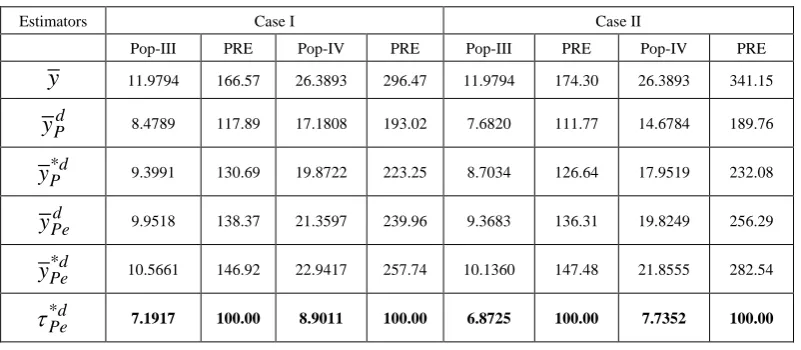
0.0458

Table-1 and Table-2 below present the mean squared errors of different ratio type and product type estimators respectively for both the cases.

5. Conclusions

In the present manuscript we have proposed two exponential ratio and exponential product type class of estimators. The biases and the mean squared errors of both the estimators have been obtained up to the first order of approximation. The optimum values of the characterizing scalars which minimize the corresponding mean squared errors have been obtained and corresponding minimum mean squared errors of these estimators have been obtained. The various conditions under which both the estimators perform better than the other ratio and product type estimators under two-phase sampling scheme have been given. A numerical study is also carried out to evaluate the performances of various ratio and product estimators along with the proposed estimators under two-phase sampling using four populations. In the first two populations, the study variable and the auxiliary variable are positively correlated. There is negative correlation in the other two populations. From Table-1 and Table-2, we see that the mean squared error of the proposed estimators



*_Red and



*_Ped respectively are smaller than the other estimators discussed here. Hence the proposed estimators may be preferred over the existing estimators.

Table 1. Mean squared error of different ratio estimators

Estimators Case I Case II

Pop-I PRE Pop-II PRE Pop-I PRE Pop-II PRE

y

168488.1 195.46 2343750 437.50 168488.1 244.49 2343750 440.88

d R

y

391542.8 454.22 2036607 380.17 1054187 1529.70 2021946 380.38 *d

R

y

538452.2 624.64 2217464 413.93 1460110 2118.72 2211264 415.96

Red

y

103853.5 120.48 2186607 408.17 183515.9 266.29 2178929 409.88 *

Re

d

y

123381.2 143.13 2280036 425.61 255511.2 370.77 2276879 428.30 *

Re

d

(7)

Table 2. Mean squared error of different product estimators

Estimators Case I Case II

Pop-III PRE Pop-IV PRE Pop-III PRE Pop-IV PRE

y

11.9794 166.57 26.3893 296.47 11.9794 174.30 26.3893 341.15

d P

y

8.4789 117.89 17.1808 193.02 7.6820 111.77 14.6784 189.76 *d

P

y

9.3991 130.69 19.8722 223.25 8.7034 126.64 17.9519 232.08

d Pe

y

9.9518 138.37 21.3597 239.96 9.3683 136.31 19.8249 256.29 *d

Pe

y

10.5661 146.92 22.9417 257.74 10.1360 147.48 21.8555 282.54 *d

Pe



7.1917 100.00 8.9011 100.00 6.8725 100.00 7.7352 100.00

Appendix

Using approximations, the proposed estimator may be written as,





















* 2 2 2 2 2 2 2

Re 0 2 1 2 1 2 1 2 2 1 2 1

1

2

4

8

d

Y

e

g e

e

e e

g

e e

e

g

e









_



 



_





 









_

_































* 2 2 2 2 2 2 2

Re 0 2 1 2 1 2 1 2 2 1 2 1

1

2

4

8

d

Y

e

g e

e

e e

g

e e

e

g

e









_

 



_



 









_

_







































2 2 2 2 2 2 2

2 1 2 1 2 1 2 2 1 2 1

*

Re 0

2 2 2 2 2 2 2

2 1 2 1 2 1 2 2 1 2 1

1

2

4

8

1

2

4

8

d

g e

e

e e

g

e e

e

g

e

Y

e

g e

e

e e

g

e e

e

g

e







_

_{  }

_

_{ }

_









_

_







_

_

_{  }

_

_{ }

_

_



_

_







Retaining the terms up to the first order of approximation, we have

























2 2 2 2 2 2 2

0 0 2 0 1 2 1 2 1 2 1 2 2 1 2 1

* Re

2 2 2 2 2 2 2

0 2 0 1 2 1 2 1 2 1 2 2 1 2 1

1 1 1

1

2 4 8

1 1 1

2 4 8

d

e g e e e e e e e e e g e e e e g e e

Y

g e e e e e e e e e g e e e e g e e





 _{ } _ _{  } _ _ _ _ _ _ 

 

  _ _

 _ _ _ _{  } _ _ _ _ _ _ _

  

 

Subtracting

Y

_{on both sides of above equation, we have}

























2 2 2 2 2 2 2

0 0 2 0 1 2 1 2 1 2 1 2 2 1 2 1

* Re

2 2 2 2 2 2 2

0 2 0 1 2 1 2 1 2 1 2 2 1 2 1

1 1 1

2 4 8

d

e g e e e e e e e e e g e e e e g e e

Y Y

g e e e e e e e e e g e e e e g e e





 _ _ _{   } _ _{ } _ _ 

 

   

 _ _ _{   } _ _{ } _ _ 

 

 

(*)

Taking expectation on both sides in above equation, we have





























2 2 2 2

0 0 2 0 1 2 1 2 1 2 1 2 2 1

* 2 2 2 2

Re 2 1 0 2 0 1 2 1 2 1 2

2 2 2 2 2 2

1 2 2 1 2 1

1 1

( ) ( ) ( ) ( ) ( ) ( ) ( ) ( ) ( ) ( )

2 4

1

( ) ( ) ( ) ( ) ( ) ( ) ( ) ( )

8 2

( ) ( ) ( ) ( ) ( )

4 8

d

E e g E e e E e e E e E e E e E e e g E e e E e E e

E Y Y g E e E e g E e e E e e E e E e E e E e e

g E e e E e E e g E e E e

 

 

 _ _ _ _ _ _ _ _ _

  

  _        

    

    

 

 

(8)

 

* 2 * 2 2 2 ** 2





Re

1

8

2

d

x x x

B





Y



_

g



C



g



C



g



CC



_









Squaring on both sides of (*), simplifying and retaining the terms up to the first order of approximation, we have,

























2

2 2 2 2 2 2 2

0 2 1 1 2 2 1 1 2 0 2 0 1

2

* 2

Re

2 2 2

0 2 0 1 2 1 1 2

1

2

4

2

d

e

g

e

e e

g

e

e e

g e e

e e

Y

g e e

e e

g

e

e e





























_

_



_

_

_







Taking expectations both the sides of above equation, we have the mean squared error of the proposed class of estimators up to the first order of approximation as,

 





















2

2 2 2 2 2 2 2

0 2 1 1 2 2 1 1 2

* 2

Re

2 2 2

0 2 0 1 0 2 0 1 2 1 1 2

1 (

)

(

)

(

) 2 (

)

(

)

(

) 2 (

)

4

4 (

)

(

)

(

)

(

)

(

)

(

) 2 (

)

2

d

E e

g

E e

E e e

g

E e

E e e

MSE

Y

g E e e

E e e

g E e e

E e e

g

E e

E e e























_

_



_

_

_

_







Putting the values of different expectations and simplifying, we have,

 

2

* 2 2 ** 2 ** 2 2 ** 2 2 ** 2

Re

1

4 4 2

d

y x x x x

MSE



Y 



C g



C _ gC_





g C 





g C 

 

g CC 

 

 

 

REFERENCES

[1] Bahl, S., & Tuteja, R. K. (1991). Ratio and Product type exponential estimator, Information and optimization Sciences,

12, 159-163.

[2] Cochran, W. G. (1977). Sampling techniques, New-York: John Wiley and Sons.

[3] Johnston, J. (1972): Econometric methods, (2nd ed.), McGraw-Hill, Tokyo.

[4] Kalita, D. and Singh, B. K. (2013). Exponential dual to Ratio and dual to Product-type Estimators for Finite Population Mean in Double Sampling, Elixir Statistics, 59, 15458-15470. [5] Kadilar, C., Cingi, H. (2006). New ratio estimators using

correlation coefficient, Interstat, 4, 1–11.

[6] Kumar, M., and Bahl, S. (2006). Class of dual to ratio estimators for double sampling, Statistical Papers, 47, 319-326.

[7] Murthy, M. N. (1964). Product method of estimation,

Sankhya, 26, 69-74.

[8] Murthy, M. N. (1967). Sampling theory and methods, Calcutta, India: Statistical Publishing Society.

[9] Neyman, J.(1938) Contribution to the theory of sampling human population, Journal of the American Statistical Association, 33, 101-116.

[10] Robson, D.S., (1957), Application of Multivariate polykays to the theory of unbiased ratio-type estimation, Journal of the American Statistical Association, 52, 511-522.

[11] Singh, B.K., Choudhury. S. (2012). Dual to Product Estimator for Estimating Population Mean in Double Sampling, International Journal of Statistics and Systems, 7,1, 31-39. [12] Singh, H. P. and Vishwakarma, G. K. (2007). Modified

exponential ratio and Product estimators for finite population mean in double sampling. Austrian Journal of Statistics, 36, 3, 217-225.