Managing complexity in high-concentration flow modelling aimed at hazard assessment: numerical and practical aspects

(1)

Doctoral School in Civil, Environmental and Mechanical Engineering Topic 1. Civil and Environmental Engineering - XXIX cycle 2014/2016 Doctoral Thesis - December 2017

Nadia Zorzi

Managing complexity

in high-concentration flow modelling

aimed at hazard assessment

Numerical and practical aspects

Supervisor Giorgio Rosatti DICAM Department of Civil, Environmental and

(2)

Except where otherwise noted, contents on this book are licensed under a Creative Common Attribution - Non Commercial - No Derivatives

4.0 International License

University of Trento

Doctoral School in Civil, Environmental and Mechanical Engineering http://web.unitn.it/en/dricam

Via Mesiano 77, I-38123 Trento

(3)

Abstract

High-concentration flows are complex phenomena typical of Alpine mountain areas. Essentially, they are free-surface flows with intense sediment transport, often caused by intense rainfall events and involving large volumes of solid material. Because of the amount of sediments moved, the intense erosion and depos-ition processes typically observed and the quite unexpected char-acter, these phenomena represent a serious hazard in populated mountain areas, where reliable and effective hazard-management and -protection strategies are required.

In mountain-hazard management, high-concentration flows modelling represents a key factor, since it allows to evaluate im-pacts of possible hazard scenarios and the effectiveness of possible protection and mitigation measures. However, the intrinsic phe-nomenon complexity makes high-concentration flow modelling and hazard assessment quite challenging. In this thesis, some of the effects of high-concentration flow complexity on modelling are experienced directly and suitable solutions are proposed, to make the phenomenon description more reliable and straightfor-ward.

Among very different modelling approaches present in the lit-erature, this work embraced the quasi-two phase, mobile-bed ap-proach proposed in Armanini et al. (2009b) and in Rosatti and Beg-nudelli (2013a), which is implemented in the TRENT2D model. TRENT2D is a quite sophisticated model that solves a system of Partial Differential Equations over a Cartesian mesh by means of a finite-volume method with Godunov-type fluxes.

(4)

then faced directly. According to the purpose of this thesis, pos-sible solutions to the issues were proposed, to ensure a proper description of the flow behaviour and possibly limit intricacy in the model use.

The first complexity issue is "operational" and regards the use of the TRENT2D model and, more in general, the amount of work necessary to perform a complete hazard-assessment job about high-concentration flows. Because of the phenomenon complex-ity and the sophisticated character of the model, the operational chain necessary to assess hazard by means of TRENT2D appears quite demanding. The large efforts required in terms of hand-work, computational charge and resources may divert the user attention from the physical meaning of the hazard-assessment process, possibly leading to inaccurate results. To overcome this issue, a possible solution is proposed, based on the use of a loosely-coupled Service Oriented Architecture approach. The aim is to develop a unique, user-friendly working environment able to support high-quality, cost-effective hazard assessment and, in perspective, the possible development of a Decision Support System for mountain hazard.

The second complexity issue is "geometrical" and "numerical" and concerns morphology representation. Because of the strong interaction between high-concentration flows and bed morpho-logy, these phenomena require bed morphology to be described with the right level of detail, especially where heterogeneity is outstanding. This is typically the case of urbanised mountain areas, with their characteristic terrain shapes, buildings, infra-structures, embankments and mitigation structures. A believable representation of these geometrical constraints may be fulfilled acting on the computational mesh used to solve model equations, preferably avoiding regular Cartesian meshes. In this work, a new version of the TRENT2D model is developed, based on the use of Delaunay, triangular unstructured meshes. To reach second-order accuracy, a MUSCL-Hancock approach is considered, with gradient computation performed by means of the multidimen-sional method proposed in Barth and Jespersen (1989) for Euler equations. The effects of different gradient limiters are also eval-uated, aiming at a proper description of the flow dynamics in heterogeneous morphology contexts.

(5)

Abstract

structures aimed expressly at controlling the high-concentration flow behaviour, attention was paid to sluice gates, which can be used in channels and hydropower reservoirs to control sediment routing. In the literature, the effects of sluice gates have been studied especially with reference to clear water flows over fixed beds, while knowledge about the influence on high-concentration flows over mobile beds is still limited. Here, a rough, bread new mathematical description is proposed, in order to take into ac-count the 3D morphodynamics effects caused by sluice gates in high-concentration flow modelling.

The last complexity issue is pretty "numerical" and arises from the challenge of numerical models to comply with the phe-nomenon complexity. Generally speaking, reliable numerical models are expected to catch the main characteristics of the phys-ical processes at both a general and a local spatial scale, although with a certain level of approximation, depending on the numer-ical scheme. Sometimes it may be hard to close the gap between the local phenomenon complexity and its numerical representa-tion, leading to non-physical numerical results that could affect hazard assessment. In this work, a particular numerical issue is investigated, which was identified through a thorough analysis of TRENT2D model results. In particular, it was observed that the direction of the numerical mixture-mass flux is occasionally opposite to the direction of numerical solid-mass flux, despite the isokinetic approach which the model is based on. This incoher-ence was studied with a rigorous method, trying to fix the source of the problem. However, the question turned out to be quite tricky, due to the sophisticated character of the model.

(6)

(7)

Everything should be made as simple as possible, but not simpler.

(8)

(9)

Acknowledgements

First and foremost, I would like to thank professor Giorgio Rosatti for the opportunity of working on such a relevant and topical subject. Beyond the scientific and technical growth which he guided me through, I would like to thank him for what I learnt about method, constancy and passion. The years I passed working with him were not simply a school of hydraulics but rather a school of life.

Secondly, I would like to thank professor Marian Muste and professor Stefano Sibilla, who were the reviewers of this thesis. I am grateful to them for their careful reading and their relevant observation, which allowed to improve the quality and the con-tents of this work. A special thanks goes also to professor Luigi Fraccarollo and his co-worker Anna Prati, whose collaboration was essential to develop Chapter 7 of this thesis. Thanks also to professor Michael Dumbser, for the tips about unstructured meshes, to Walter Bertoldi, for the encouragement to reflect about complexity, and to Valentina Cavedon, who (unwittingly) gave me the last little push necessary to opt for this experience.

I would like to thank all my colleagues, or rather friends, who I work with in these years. A special thanks goes to Daniel, who was a constant, reassuring and helpful presence during all this path. Thanks also to Michele, Laura, Daniel, Cristian, Simona, Marta, Erika, Stefano, Alessandro, Andrea and Davide, for shar-ing with me some steps of the path. I was pleased to work with them, who made me feel at home at any time. Thanks also to Oscar, who was used to remind me that acknowledgements are the most demanding part of the thesis (and he was right).

(10)

I want to thank my parents, who were the essential point of reference during these years and accompanied my experience with a lot of encouragements and wise advices. Thanks also because they educate me to perseverance, diligence, patience and uprightness.

A special thanks goes to Fabiano, who was my energy when I was tired, my hope when I was disheartened, my happiness when I was cheerful and my faithful window onto the world. Thanks also to his family, whose warmth is extraordinary. Thanks to my friends of the "Blue van" group, for never giving up to encourage me and remind that true life is made of a lot of little, special moments and intermediate goals. Thanks also to the girls of the "Mater armata", for bringing music, which is a part of my life, inside my office.

(11)

Contents

List of Figures

1.1 Rheological behaviours typical of high-concentra-tion flows (from Armanini et al., 2005): (a) imture or oversaturated flow over loose bed; (b) ma-ture flow over loose bed; (c) unsaturated flow over loose bed; (d) flow over rigid bed. . . 7 1.2 Erosion due to a debris flow event (Valle

Molin-ara, Italy) Courtesy of the Autonomous Province of Trento. . . 8 1.3 A debris flow over an alluvial fan: Campolongo di

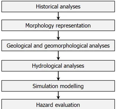
Piné, 15th August 2010. Courtesy of the Depart-ment for Territory, Agriculture, EnvironDepart-ment and Forestry of the Autonomous Province of Trento . . . 9 1.4 Main steps of the procedure typically used in

moun-tain-flow hazard assessment . . . 11

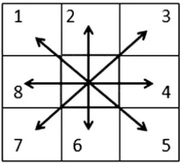
2.1 Basic notation used to write the 1D, mono-phase model equations . . . 24 2.2 Scheme of the eight possible flow directions

con-sidered in Gregoretti et al. (2016) . . . 26 2.3 Basic notation used to write the 1D, QTP model

equations . . . 28 2.4 Basic notation used to write the 1D, FTP model

equations . . . 31 2.5 From Toro (2009): simple wave solutions of the RP:

(a) shock wave, (b) contact wave, (c) rarefaction wave 33

3.1 Reference system and control volume used to write the TRENT2D model equations (Rosatti and Beg-nudelli, 2013a) . . . 44

(16)

4.2 Rainfall heights measured by the Sant’Orsola Terme rain gauge from 14th August 2010 2:00 pm to 15th August 6:00 am (UTC+2) . . . 62 4.3 (a) Erosion and (b) deposition in Valle Molinara

basin after the 2010 debris-flow event. Courtesy of the Autonomous Province of Trento . . . 63 4.4 Deposition depths and volumes surveyed by the

local agency of the Autonomous Province of Trento over the Valle Molinara alluvial fan. Courtesy of the Autonomous Province of Trento. . . 64 4.5 Rainfall heights measured by the Sant’Orsola Terme

rain gauge from (histogram) and liquid discharges produced by PeakFlow for the Valle Molinara basin closed at the fan apex (UTC+2). . . 66 4.6 3D representation of the terrain elevation inside

the computational domain used in the "blind" re-construction of the Valle Molinara event . . . 67 4.7 Deposition area on the Campolongo fan computed

through the TRENT2D back-analysis, compared to the real deposition area, delimited according to field surveys and aerial pictures . . . 69 4.8 Mixture discharges (hatching) and solid discharges

(dots) estimated blindly for the Valle Molinara debris-flow event (UTC+2) . . . 70 4.9 A local detail of the optimal simulation . . . 73 4.10 Erosion and deposition depths at the end of the

op-timal simulation reconstructing the Valle Molinara event . . . 74 4.11 (a) Rio Lazer in the basin of the Cismon stream

(Lenzi and Paterno, 1997) (b) Perimeter of the Rio Lazer basin (red) and its alluvial fan (green) . . . 77 4.12 Rainfall heights measured by the rain-gauge of

Tonadico (Italy) in October and November 1966: daily heights (above) and cumulative heights (be-low) . . . 78 4.13 Precipitation measured by the rain-gauge of

Ton-adico (Italy) in between the 1stand the 7thof Novem-ber 1966: daily average rainfall intensity (above) and cumulative rainfall height (below) . . . 79 4.14 Picture representing Rio Lazer and the inundated

(17)

List of Figures

4.15 Map of areas interested by the 1966 event in the Rio Lazer basin (Lenzi and Paterno, 1997): erosion (purple), reactivated landslides (pink), deposition area (yellow) and interrupted roads (blue) . . . 80 4.16 Hydrographs hull obtained by means of PeakFlow

considering the six synthetic hydrographs produced for the Rio Lazer basin . . . 82 4.17 DTM modifications over the Rio Lazer alluvial fan:

(a) original DTM surveyed in 2008; (b) addition of 1966 buildings p(rectangles) and deletion of the two bridges (circles); (c) editing of the current de-position basin; (d) editing of the plain above Siror street. . . 85 4.18 Maps of simulated erosion and deposition depths

at the end of the simulations with rainfall duration of (a) 1h; (b) 2h; (c) 3h; (d) 4h; (e) 5h; 6h. . . 86 4.19 Map of erosion and deposition depths at the end

of the Rio Lazer simulation, based on a rainfall duration of 3h, over-layered to the perimeter of the flooded area indicated in Lenzi and Paterno (1997). 87 4.20 Detail of the deposition area on the left bank of Rio

Lazer. . . 88

5.1 Logo and acronym of WEEZARD . . . 101 5.2 Logical architecture of the WEEZARD solution . . . 102 5.3 Component diagram describing the physical

archi-tecture of the WEEZARD solution . . . 103 5.4 System development life cycle applied for the

WEEZ-ARD development . . . 105 5.5 Main window of the WEEZARD system . . . 109 5.6 Main menu for accessing the WEEZARD

function-alities . . . 110 5.7 Tabs of theDTMmenu in WEEZARD . . . 110 5.8 Three-panel window ofEdit cellsin WEEZARD . . . 111 5.9 Definition of a computational domain in WEEZARD112 5.10 Computational domain in WEEZARD: (a) Selection

(18)

5.15 3D-view framework in WEEZARD . . . 118

5.16 Analyze mappanel in WEEZARD . . . 119

5.17 Scheduling queue window in WEEZARD . . . 120

5.18 WEEZARD administrative panel . . . 121

5.19 BUWAL matrix . . . 122

5.20 Flowchart describing the hazard-level mapping job and the intermediate outputs. In WEEZARD it is performed automatically by the Hazard Mapper module. . . 124

5.21 Hazard-level map (HYP1) obtained through WEEZ-ARD for the Valle Molinara alluvial fan, consider-ing the liquid hydrographs with the highest peak discharge. . . 126

5.22 Hazard-level map (HYP1) obtained through WEEZ-ARD for the Valle Molinara alluvial fan, consider-ing rainfall durations of (a) 45 minutes and (b) 120 minutes. . . 127

5.23 Comparison between the extent of the hazard-level map (HYP1) obtained through WEEZARD for the Valle Molinara alluvial fan (rainfall duration of 45 minutes) and the deposition area surveyed after the 2010 event (in light yellow). . . 128

5.24 Layout of methodologies involved in a end-to-end, generalized DSS and their interactions, from Muste and Firoozfar (2016) . . . 131

6.1 Meshes: (a) domain to be meshed; (b) coarse Carte-sian mesh; (c) fine CarteCarte-sian mesh; (d) block-structured mesh; (e) cut-cell mesh; (f) unstructured mesh . . . 135

6.2 (a) Circumcircle property (b) Voronoi diagram . . . 138

6.3 Notations and conventions used in the unstruc-tured mesh management . . . 139

6.4 Compact support used to compute the gradient ac-cording to Barth and Jespersen (1989) . . . 144

6.5 TRENT2D-UTG uniform-flow test with Barth and Jespersen (1989) limiter computed at (a) verticesm (b) edge midpointsM(c) intersectionsP . . . 149

(19)

List of Figures

6.7 TRENT2D-UTG uniform-flow test with Venkatakrish-nan (1995) limiter computed at (a) edge midpoints M(b) intersectionsP . . . 150 6.8 Results obtained through TRENT2D-UTG for the

test with three rarefaction waves, applying the Barth and Jespersen (1989) limiter computed at intersec-tionsPover a mesh of 51200 cells: (a) free surface and bed elevation; (b) velocity along the main flow directionxand Froude number . . . 151 6.9 Comparison of the five different approaches

avail-able in TRENT2D-UTG for limiter computation, considering the three-rarefaction test and a grid with 51200 cells . . . 152 6.10 Zoom on results obtained through TRENT2D-UTG

for the test with three rarefaction waves, apply-ing the different limiter computations over a mesh of 15492 cells: (a) Barth and Jespersen (1989) ap-proach; (b) Venkatakrishnan (1995) approach . . . . 152 6.11 Comparison of results obtained by means of

TRENT2D-UTG with the Barth and Jespersen limiter computa-tion at interseccomputa-tions, considering the three-rarefaccomputa-tion test and six different meshes . . . 153 6.12 Zoom on the comparison of results obtained by

means of TRENT2D-UTG with the Barth and Jes-persen limiter computation at intersections, con-sidering the three-rarefaction test and six different meshes . . . 153 6.13 Results obtained through TRENT2D-UTG for the

test with two rarefaction waves and one shock, ap-plying the Barth and Jespersen (1989) limiter com-puted at intersectionsPover a mesh of 1549 cells: (a) free surface and bed elevation; (b) velocity along the main flow directionxand Froude number. . . . 154 6.14 Comparison of the five different approaches

(20)

6.15 Zoom on the shock representation obtained through TRENT2D-UTG for the test with two rarefaction waves and one shock, applying the different limiter computations over a mesh of 15492 cells: (a) Barth and Jespersen (1989) approach; (b) Venkatakrish-nan (1995) approach . . . 155 6.16 Comparison of results obtained for the same RP by

means of TRENT2D and TRENT2D-UTG consider-ing grids with the same number of cells . . . 157 6.17 Zoom on the third rarefaction wave in the results

comparison for the same RP by means of TRENT2D and TRENT2D-UTG considering grids with the same number of cells . . . 157 6.18 3D view of the circular dam-break results att =3 s

(centroid values). . . 158 6.19 2D view of the circular dam-break results att=3 s:

(a) 2D view in the (x,y) plane (centroid values); (b) 2D view in the (x,z) plane (centroid values). . . 158 6.20 3D view of the reservoir morphology. . . 159 6.21 3D view of the unstructured mesh used to discretise

the reservoir morphology. . . 160 6.22 (a) 3D and (b) 2D view of the unstructured mesh in

the refined area . . . 161 6.23 Location of the boundary conditions set for the

hydropower-reservoir domain. . . 162 6.24 Mixture hydrograph supplied at the inflow

sec-tion of the hydropower reservoir for the sediment-routing test with TRENT2D-UTG . . . 163 6.25 (a) Initial and (b) final condition of the bed

eleva-tion of the reservoir before and after the TRENT2D-UTG simulation . . . 163 6.26 Erosion (blue) and deposition (red) depths in the

reservoir after the TRENT2D-UTG simulation . . . 164 6.27 Erosion (blue) and deposition (red) depths in the

refined area near the reservoir outlet: center cell values for (a)t=6h, (b)t=12h, (c)t=18hand (d) t=29h. . . 165

7.1 Sluice gates of the Stramentizzo dam (Italy). . . 168 7.2 Typical internal flow structure upstream the sluice

(21)

List of Figures

7.3 Horseshoe vortex upstream the sluice gate: (a) sketch edited from Montes (1997); (b) side view from Speerli et al. (1999) . . . 170 7.4 Sluice gate notation. . . 171 7.5 Bed (brown) and free-surface (light blue) profiles

observed during the high-concentration sluice-gate flow experiments in steady-state condition. Cour-tesy of prof. Fraccarollo. . . 176 7.6 Bed profile observed upstream a slit check dam.

Pricture edited from Armanini and Larcher (2001). . 176 7.7 Gate lifting experiment with sand: from (a) a partial

opening to (h) a total opening. Courtesy of Anna Prati. . . 177 7.8 Bed profile near the sluice gate: experimental data

(PVC) and their interpolation . . . 178 7.9 Comparison between Cq values obtained

experi-mentally for gate-controlled high-concentration flows over mobile bed and estimates computed accord-ing to formulations of Table 7.1: percentage relative error of the PVC set of experiments. . . 181 7.10 Schematisation of a gate-controlled high-concentration

flow in steady-state condition over a mobile bed. The hatched line bounds the control volume used in the computations. . . 182 7.11 Gate manoeuvre: gate openings in time. . . 187 7.12 (a) Initial and (b) final condition of the bed

eleva-tion of the reservoir before and after the TRENT2D-UTG simulation with gate control . . . 188 7.13 Bed elevation inside the reservoir, after the

TRENT2D-UTG simulation (a) without gate control and (b) with gate control . . . 189 7.14 Erosion (blue) and deposition (red) depths in the

reservoir, after the TRENT2D-UTG simulation (a) without gate control and (b) with gate control. . . . 190 7.15 Hydropower reservoir: inflow and outflow

hydro-graphs, obtained for the simulations without and with gate control. . . 190 7.16 Cumulative volume of outflow sediments, obtained

(22)

7.17 Erosion (blue) and deposition (red) depths in the refined area near the reservoir outlet in the gate-controlled case: center cell values for (a)t=6h, (b) t=12h, (c)t=18hand (d)t=29h. . . 191

(23)

List of Tables

3.1 Parameters of the TRENT2D model . . . 58

4.1 A-priori values chosen for the PeakFlow paramet-ers to study the 2010 debris-flow event of Valle Molinara . . . 65 4.2 Relevant quantities characterising the five

concen-tration scenarios considered in the Valle Molinara back-analysis . . . 67 4.3 A-priori values chosen for the TRENT2D

paramet-ers in the Valle Molinara event reconstruction . . . . 67 4.4 βvalues considered in the back-analysis of the Valle

Molinara debris flow. . . 68 4.5 Y values considered in the back-analysis of the

Valle Molinara debris flow. . . 68 4.6 A-priori values chosen for the TRENT2D

paramet-ers in the Valle Molinara blind simulation . . . 70 4.7 A-priori values chosen for the PeakFlow parameters 82 4.8 Liquid volumes of the six liquid hydrographs

ob-tained for the back-analysis of the Rio Lazer event . 82 4.9 Concentration, amplification factor and mixture

vo-lume values for the six synthetic hydrographs ob-tained for the Rio Lazer back-analysis . . . 83 4.10 A-priori values chosen for the TRENT2D

paramet-ers in the Rio Lazer back-analysis . . . 84 4.11 Values of the transport parameterβfor the six

syn-thetic scenarios considered in the Rio Lazer back-analysis . . . 86

(24)

6.1 Numerical convergence results obtained for the three-rarefaction test with TRENT2D-UTG and the Barth and Jespersen limiter computation at inter-sections. . . 153

7.1 Some literature formulations for the sluice-gate dis-charge coefficientCq. . . 173

(25)

List of Tables

List of symbols

α [◦

] Slope angle ;

αgate [◦] Bed slope angle near the sluice gate ;

β [-] Transport parameter ;

βr [-] Reference transport parameter ;

∆l [L] Characteristic length of mesh cells ;

∆t [T] Timestep ;

∆x [L] Cell size alongx-axis ;

∆y [L] Cell size alongy-axis ;

∆z [-] Bed slope height near the sluice gate ;

∆z [L] Bed step height near the sluice gate ;

∆ [-] Submerged relative density ;

λ [-] Linear concentration ;

λi i-th eigenvalue ;

λmax Maximum eigenvalue ;

λmin Minimum eigenvalue ;

5_W_n _{Primitive gradient ;}

Λ Eigenvalues matrix ;

Φ Vector of primitive variable limiters ;

˜

D Vector of non-conservative terms ;

e

Wn Vector of averaged primitives alongndirection ;

(26)

An Roe matrix ;

B GR-matrix ;

Bn Roe matrix ;

Dn vector of the non-conservative terms ;

F Vector of the numerical fluxes ;

F Vector of fluxes inxdirection ;

FHLL _{Vector of HLL-fluxes ;}

Flat _{Vector of lateral fluxes ;}

FLHLL _{Vector of LHLL-fluxes ;}

Fn Vector of fluxes along thendirection ;

G Vector of fluxes inydirection ;

Hn Matrix of non-conservative terms ;

JFn Jacobian matrix of the fluxesFn;

JUn Jacobian matrix of the conserved variablesUn;

JF Jacobian matrix of fluxes ;

M Rotation matrix ;

n Unit normal vector ;

R Eigenvectors matrix ;

Ri i-th eigenvector associated to thei-th eigenvalue ;

t Unit tangential vector ;

Tn Vector of source terms along thendirection ;

U Vector of the conserved variables ;

Un Vector of conserved variables alongndirection ;

Wn Vector of primitive variables alongndirection ;

wn Component of the primitive gradient ;

A _{Global GR-matrix ;}

A_n _{Roe matrix ;}

(27)

List of Tables

φ [◦

] Friction angle ;

Ψ [-] Function for gradient limiter computation ;

ρm [ML−3] Mixture density ;

ρs [ML−3] Solid-phase density ;

ρw [ML−3] Liquid-phase density ;

τbc [ML−1T−2] Critical bed shear stress ;

τbx [ML−1T−2] Bed shear-stress inx-direction ;

τby [ML

−₁

T−2_{] Bed shear-stress in}_y_{-direction ;}

τs [ML

−₁

T−2_{] Shear stress of the solid phase ;}

τw [ML

−₁

T−2_{] Shear stress of the liquid phase ;}

~τb [ML

−1_T−2_{] Bed shear-stress vector ;}

~

u [LT−1] Depth-average velocity vector ;

A [L2_] _{Cell area ;}

a [-] Bagnold constant ;

a [L] Gate opening ;

c [-] Depth-average concentration ;

cb [-] Maximum bed packaging concentration ;

Cc [-] Contraction coefficient ;

Cq [-] Discharge coefficient ;

CFL [-] Courant coefficient ;

D [L2_T−1_] _Coe_ffi_{cient of hydrodynamic dispersion ;}

D [LT−1_] _{Sediment deposition flux ;}

D [L] Deposition depth ;

d [L] Grain size ;

D0 [L3T

−2_] _{Bed pressure term ;}

di [L] Incircle diameter ;

E [LT−1] Sediment erosion flux ;

(28)

Fa [-] Amplification factor ;

g [LT−2] Gravitational acceleration ;

h [L] Flow depth ;

h0 [L] Undisturbed flow depth ;

Hl [-] Hazard level ;

i [-] Intensity ;

iF [-] Bed slope ;

iF,gate [-] Bed slope near the sluice gate ;

k [-] Constant ;

Ks [L1/3T−1] Gauckler-Strickler roughness coefficient ;

L [-] Subscript for left states or fluxes in a RP ;

M Edge midpoint ;

m Magnitude ;

m0 Threshold magnitude ;

P Intersection of edge and centroid-centroid segment

;

P [-] Occurrence probability ;

p [-] Porosity ;

q [L2_T−1_] _{Discharge per unit width ;}

Qliq [L3T

−1_] _{Liquid-phase discharge ;}

Qmix [L3T−1] Mixture discharge ;

qmix [L2T−1] Mixture discharge per unit width ;

Qsol [L3T−1] Solid-phase discharge ;

qsol [L2T

−1_] _{Solid-phase discharge per unit width ;}

R [-] Subscript for right states or fluxes in a RP ;

S Wave velocity in a Riemann Problem ;

S [-] Percentage of saturated basin area ;

(29)

List of Tables

SR =min(λmax,L, λmax,R) ;

t [T] Time ;

uc [LT

−₁

] Channel velocity ;

uh [LT−1] Hillslope velocity ;

un [LT−1] Normal velocity ;

us [LT−1] Velocity of the solid phase ;

ut [LT

−1_] _{Tangential velocity ;}

uw [LT−1] Velocity of the liquid phase ;

ux [LT−1] x-component of depth-average velocity ;

uy [LT−1] y-component of depth-average velocity ;

v [LT−1_] _{Velocity absolute value ;}

Vmix [L3] Mixture volume ;

Vsol [L3] Solid-phase volume ;

X [L] Gate-controlled length along the flow direction ;

x [L] x-horizontal coordinate ;

Y [-] Relative submergence ;

y [-] Dummy variable for limiter computations ;

y [L] y-horizontal coordinate ;

z [L] z-vertical coordinate ;

(30)

(31)

1. High-concentration flow hazard assessment: complexity, simplicity and complicatedness

Chapter 1

High-concentration flow

hazard assessment:

complexity, simplicity and

complicatedness

Natural hazard assessment is a key factor in disaster manage-ment. Any efficient protection or mitigation strategy can not be planned without accurate and reliable hazard assessment. How-ever, natural hazard assessment may be not straightforward, for two main reasons: the intrinsic complexity of natural hazard-ous phenomena and the effects of this complexity on the hazard-assessment procedural chain, which compulsory includes a wide heterogeneity of information and operations.

Undeniable complexity of natural hazards hinders signific-antly their knowledge and understanding. However, despite the type, the number and the mutual connections of relevant nat-ural entities and processes to be considered, understanding is mandatory to lead reliable hazard assessment, although quite de-manding.

(32)

possible, i.e. avoiding complicated operations and outcomes. In this work, this challenge is taken up with reference to a particular class of flow-like hazardous phenomena, characteristic in mountain regions and indicated hereafter as high-concentration flows. These phenomena and their complexity are described in Section 1.2, while Section 1.3 pertains to the effects of complexity over the hazard-assessment process.

However, before discussing about high-concentration flows, it is convenient taking a bearing about the meaning of the word complexity, in order to understand properly its nuances and to frame the purpose of this work clearly. For this reason, in Section 1.1, an etymological analysis is proposed, not only about the term complex, but also considering other strictly-related terms.

1.1

Some definitions

The concept of complexity belongs to the common way of speaking and, at first sight, its meaning appears plain and in-tuitive. Complexis something that is not easily understandable. Similarly, also concepts ofsimpleandcomplicatedappear plain and intuitive: simple is the opposite of complex, while complicated is often interpreted as a synonym ofcomplex.

This is confirmed by the definitions proposed by the Oxford English Dictionary:

- simple: easily understood or done;

- complex: consisting of many different and connected parts; not easy to analyse or understand;

- complicated: consisting of many interconnecting parts or ele-ments.

However, over the years these terms have been used in a number of different ways, not only in the field of environmental sciences but also in physics, informatics, business management, social sciences, policy sciences (Gell-Mann, 1995). For this reason, their etymology is here investigated, in order to disclose some important shades and ensure the right interpretation of these three terms along the entire work.

(33)

1.1. Some definitions

connecting". Therefore,simpleis something that is plain, made of a single part and, so, it can be understood immediately.

Simpleshares withcomplexthe rootplex-that, incomplex, comes after the other Latin prefixcum-, which means "together" and im-plies "many", as clearly explained in Gell-Mann (1995) and in Sun et al. (2016). Therefore, complex indicates something that is made of many interconnected parts. What makes something complex is not only the quantity of parts, but also their mutual relationships, their links. Somethingcomplex can not be under-stood straightforwardly, not only because of the number of parts, but also because of the number of connections. If connections are identified or mapped for the most part, understanding the overall system behaviour could become more accessible. However, a de-tailed explanation about how each element or connection works remains intrinsically out of reach, since elements and connections they can not be studied separately (Bar-Yam, 1997).

On the other side,complexandcomplicatedshare the common Latin rootcum-(Sun et al., 2016), butcomplicatedis completed by the Latin verbplicare, which is similar toplectere, but suggests that parts are "folded up" repeatedly. Complicated systems are made of many parts, which are individually simple but collectively en-tangled. This makes system understanding not straightforwardly. In other words,complicatedseems to recall some idea of mess, of intricacy. Single parts of a complicated system could be easily and completely understood if considered one at a time, but un-derstanding of the behaviour of the overall system when these parts are put all together could result unreachable.

On the basis of these shades of meaning, the explanation for how the termssimple,complexandcomplicatedare adopted in this work is the following:

- simpledoes not need any additional specification. Its com-mon meaning is suitable also in the context of this work;

(34)

- complicatedis used to characterise systems that are made of simple parts, i.e. parts that can be individually understood, but appears ravelled when parts are considered all together. A complicated system is twisted and not easily manageable, but, with significant effort, it can be made simple.

Complexity represents the essence of natural systems, therefore it can not be removed. The only things that can be done with complexity are understanding it as much as possible and describ-ing it with proper approaches that are as much simple as possible, avoiding complicatedness. These two aspects are discussed in the next Sections with reference to high-concentration flows, which are complex natural phenomena typical of mountain regions.

1.2

A not-exhaustive account about

high-concen-tration flow complexity

This Section brings into focus complexity of high-concentration flow phenomena, which knowledge is mandatory to develop re-liable descriptions to be used in mountain hazard assessment.

(35)

1.2. A not-exhaustive account about high-concentration flow complexity

to indicate the entire phenomenon, from the initiating slide to the deposition processes on alluvial fans. According to this last approach, in this work the termhigh-concentration flowis used to indicate the whole family of flow-like movements characterised by quite high-concentration values at some point of their space and time evolution. The termhigh-concentration flowis sometimes interchanged with the term mountain flows, which is used to in-dicate the same class of phenomena, but emphasizing the context where they are typically observed, i.e. mountain regions.

This work considers a quite wide range of high-concentration flow-like mass movements, which characteristic sediment con-centration can vary roughly from 1−_{2% to 40}−_{50%. Since the}

focus is set especially on mountain flows observed in the Alps, phenomena with cohesive behaviour, as for example mud flows or clay flow slides, are here excluded (their rheological behaviour is rather different from that of phenomena involving loose, coarse sediments). Mountain flows which this thesis refers to are ob-served typically in small (<5 km2) and steep basins. They are originated by intense rainfall events (sometimes also snowmelt) over saturated soils, in areas where a certain amount of coarse (but sometimes also fine), loose sediments is available. Such flows are driven by gravity (Takahashi, 2007) and can reach high velo-city (up to several meters per second), travelling long distances (Armanini, 2015). All these factors determine a great damaging potential, which becomes evident when mountain flows reach urbanised areas.

Hereafter, some aspects of natural complexity of high-concen-tration flow are shortly disclosed.

1.2.1 Solid-liquid mixture

Sediment volumes involved in a high-concentration flow can be very large if compared to the solid-transport phenomena typ-ical of floodplains. Because of sediments, the global flow rate of a high-concentration flow can exceed the runoff flow rate even by one order of magnitude. This amplification effect can be eas-ily quantified as shown in (Takahashi, 2007). Indicating with Qliq the runoff discharge and Qmix the total flow rate of a

high-concentration flow, the following relation can be set

(36)

where Fa represents the amplification factor, defined as follows

(Hashimoto et al., 1978):

Fa = cb

cb−c

(1.2)

withcrepresenting the volumetric sediment concentration andc_b representing the maximum packaging concentration of the sedi-ments in the bed. Whenever concentrationcapproachescb, the

amplification factor, and therefore the total flow rate, increases significantly. Evidently, such a discharge amplification can not be overlooked when high-concentration flows are studied, even if estimating liquid and total discharges is far from being simple. For this purpose, both hydrological and geological evaluations should be carried out, as described in Sections 1.3.4 and 1.3.5.

However hydrological analyses can be seldom based on obser-vations, since only few mountain basins are instrumented. Typic-ally, instrumentation is installed only if relevant mountain-flows are observed with very high frequency and damaging potential. Therefore, characterising the discharge evolution in time is not free from uncertainty. A few studies (for example Honglian and Xiangxing, 1988; Takahashi, 2007) and experience (personal com-munication of prof. Aronne Armanini) suggest that precipitation events causing mountain flows can be characterised by a sequence of multiple rainfall peaks, each one with different duration and intensity. However, so far, there is not a univocal characterisation of such peaks.

(37)

1.2. A not-exhaustive account about high-concentration flow complexity Figure 1.1: Rheological

behaviours typical of high-concentration flows (from Armanini et al., 2005): (a) immature or oversaturated flow over loose bed; (b) mature flow over loose bed; (c) unsaturated flow over loose bed; (d) flow over rigid bed.

What is more, the presence of both water and relevant rates of sediments that are poorly-sorted (Takahashi, 2007) requires a proper and detailed description of the rheological behaviour of the solid-liquid mixture. Because of the high sediment concen-tration, theories and methodologies developed for bed load and suspended load are not suitable for high-concentration flows (es-pecially for debris flows) (Armanini, 2013), since sediments are active players in determining resistance, both frictional and col-lisional (see Figure 1.1). Then, different and more elaborated ap-proaches have to be resorted to describe properly the two-phase dynamics. This point of discussion is further expanded first in Section 1.3.6 and then in Chapter 2.

1.2.2 Interaction with the bed

Another factor of natural complexity of high-concentration flow is their strong interaction with bed and, in general, with morphology, introducing significant modifications. It must be specified that the term bed indicates here the bound at rest co-inciding with the surface separating the (moving) flow from the motionless part of the solid-liquid mixture, as explained in Rosatti and Zugliani (2015).

(38)

Figure 1.2: Erosion due to a debris flow event (Valle Molinara, Italy) Cour-tesy of the Autonomous Province of Trento.

1.2.3 Time and space scales

As far as morphology is concerned, it must be highlighted that mountain morphology is itself complex, because of the succes-sion of hills, gullies, plains, valleys, geomorphic scars, branched stream networks, alluvial fans, etc. The heterogeneity of moun-tain morphology has a strong influence on the flow path, whether the flow is confined in a channel or not. Therefore, mountain flows should be studied with a quite detailed representation at the small scale, in order to catch point-wise flow response to the local morphology.

(39)

1.2. A not-exhaustive account about high-concentration flow complexity

Figure 1.3: A debris flow over an alluvial fan: Campolongo di Piné, 15th August 2010. Cour-tesy of the Department for Territory, Agricul-ture, Environment and Forestry of the Autonom-ous Province of Trento

1.2.4 A recent history

Evidently, studying high-concentration flows is not an easy task, because of these and also other complexity factors, which are closely related to the nature of the phenomenon. Moreover, it must be noticed also that the history of research around mountain flows is quite short in comparison with that one of large river hy-draulics. The interest around mountain flows has become more evident only in the last decades, probably because of increased frequency and size of disastrous consequences in mountain re-gions (Ammann, 2006). Therefore, mountain-flow knowledge is still quite limited and historical analyses contribute with difficulty to bridge the gap (see Section 1.3.2). Limited knowledge entails limited understanding, which contributes to the perception of mountain-flow complexity as very sizeable.

In mountain regions, and especially on alluvial fans, urbanisa-tion processes have become more frequent only in the last years. Therefore, exposition of people, buildings and infrastructure to relevant levels of hazard is quite recent (Figure 1.3 shows the debris-flow event observed in 2010 in the Molinara Valley (Italy) that damaged the urbanised alluvial fan of Campolongo, which had been uninhabited until the 1950s) and the evaluation of the possible effects of such exposition is still rough.

(40)

high-concentration flow prediction and modelling appear uncer-tain, also because they depend on a variety of rapidly evolving factors, which have been studied only in the last decades.

What is more, several basins show their hazard-prone char-acter not so frequently, i.e. every some decades or even century. This makes difficult both measurements and proofs collection. Be-sides, low event frequencies lead often to a false sense of security in local citizenry, encouraging then urban development.

1.3

How high-concentration flow complexity

af-fects hazard assessment

High-concentration flow hazard assessment requires in-depth knowledge not only of the phenomenon physics (whose complex-ity was discussed in the previous Section), but also of the study area and of any past events (when available). Moreover, it should take into account possible future scenarios of hazard and exposi-tions. Describing each on of these elements with the right level of detail may be a challenging and laborious task, sometimes leading to complicatedness. However, avoiding complicatedness is one of the duties in hazard assessment, in order to preserve assess-ment reliability. Therefore, finding theright levelof detail in each one of the procedural steps of hazard assessment is mandatory.

(41)

1.3. How high-concentration flow complexity affects hazard assessment

Figure 1.4: Main steps of the procedure typic-ally used in mountain-flow hazard assessment

1.3.1 The question of theright leveland the Occam’s razor principle

It is well-known that, to describe nature, it is necessary to re-sort to abstraction, i.e. simplification (Favis-Mortlock, 2013) of the real system. Abstraction depends much on human perception (Mulligan and Wainwright, 2013) and, generally, environmental-system complexity is perceived as too large for a thorough math-ematical representation, i.e. for extremely detailed quantitative descriptions (Beven, 2009). Therefore, complex natural systems are represented by scientist not exactly, but rather with theright levelof detail, resorting to suitable simplification when possible.

However, identifying which is theright levelis far from being simple. If the level is too much low, one runs the risk of work-ing with "spherical cows" (Harte, 1988). Otherwise, if the level is rightbut the steps required to get it are too many and too much intricate, one could end up with unsuitable or incomprehensible descriptions, which are nothing but the outcome of complicated-ness.

(42)

not univocal and depends largely on the goal of the description (Casti, 1979).

In this work, high-concentration flow description is aimed at hazard assessment, which typically involves different natural aspects, several operational issues and different scientific know-hows. In this case, an acceptable trade-off between complexity and simplification should combine enough accuracy in represent-ing the process dynamics and a desirable simplicity in readrepresent-ing results and uncertainty, compulsorily avoiding both oversimpli-fication ("spherical cows") and complicatedness.

Here, the term description is mainly referred to modelling, which is intended, broadly speaking, as the totality of operations necessary to reproduce high-concentration flow virtually. There-fore, not only models are considered here, but also field data, data representation, model use, processing efforts. For each one of these elements, undeniable requirements in terms of details and possible compromises in high-concentration flow complexity description are discussed.

(43)

1.3.2 Historical analyses

The hazard assessment process should start with historical analyses, oriented to disclose possible information about past events in the study area and, more in general, to acquire in-depth knowledge of high-concentration flow behaviour in the area. For this purpose, records, inventory, pictures, satellite imagery, chron-icles, witnesses have to be consulted carefully. In addition, on-site measurements must be collected whenever available.

Historical databases of field measurements, i.e. rain gauged data or discharge measures, are typically rare. They are available only for specific sites (among others, see Zhang, 1993; Berti et al., 2000; Marchi et al., 2002; Bacchini and Zannoni, 2003; Hürlimann et al., 2003; Mathys et al., 2003; Rickenmann and McArdell, 2007; Coe et al., 2008), prone to high-concentration flows on a yearly basis, while, as a rule, not only observations, measures and proofs, but also pictures or eyewitness memorandums are quite uncom-mon. This scarce availability of past, complete information makes phenomenon prediction and knowledge challenging and hinders hazard assessment.

However, historical analyses should pay attention not only to measurements, but also to site morphology, urbanisation evol-ution, possible presence of protection and mitigation measures and, not least, the soundness of the available documentation. The job of looking for such information does not appear as much complex, but it may become rather complicated, because of some effort required to find and validate information sources. Often, they are made available by different, not interconnected offices of public administration. Moreover, their level of detail could be not completely satisfying for hazard-assessment purposes, especially if dated documentation is investigated, and sometimes conflicting information is found.

If information is scarce or rough, any hypothesis about pos-sible past and future scenarios is barely stated and any analysis is affected by large uncertainty. This topic was tackled directly in the study proposed in Section 4.2, accounting for the back-analysis of a historic debris-flow event.

1.3.3 Morphology representation

(44)

site morphology through field surveys. The relevance of a de-tailed, although complex, representation of the site morphology was already highlighted in the previous Section. Nowadays, de-tailed representations of morphology are facilitated by the large availability of terrain information, due especially to the rapid dif-fusion reached in the last two decades by airborne and terrestrial LIDAR techniques (Roering et al., 2013). LIDAR (Light Amp-lification by Stimulated Emission of Radiation) allows to collect accurate, high-resolution elevation data, covering large areas rap-idly and also with rather high frequency. Such elevation data are gathered in Digital Elevation Models (DEMs) and Digital Terrain Models (DTMs), which represent the morphological basis to be used in modelling aimed at hazard assessment. The spatial res-olution of recently-surveyed DEMs and DTMs can be quite fine (∼₀._{5–1 m), therefore terrain features can be simply recognised}

with high, point-wise accuracy. DEMs, DTMs and other similar topographic products lighten significantly the fieldwork and al-low to improve its quality. However, fieldwork is still necessary, especially to verify the correct representation of some key, com-plex local areas and to refine accuracy of DEMs and DTMs. For this reason, LIDAR and field surveys should be considered al-ways jointly to ensure theright level of detail in the description of terrain elevation. A low level of detail or a bad representation of a heterogeneous mountain morphology could dramatically de-crease the level of accuracy and reliability of hazard-assessment jobs.

(45)

signific-1.3. How high-concentration flow complexity affects hazard assessment

antly conditioned.

Moreover, hazard-assessment analyses could require different levels of detail in different areas, which means that the spatial resolution could be not compulsory constant. Managing such heterogeneous information could be complicated, whether the point of view of model developers or practitioners is assumed. This subject is one of the main topics of this thesis, so its further discussion is postponed until Chapters 5 and 6.

1.3.4 Geological and geomorphological analyses

Next to morphology, also site geology and geomorphology require a proper level of knowledge, in order to ensure a reliable hazard assessment.

Geological investigations are necessary especially to charac-terise sediments availability in the study basin. Knowing the amount of available loose solid material, its nature and its grain-size distribution, supports the estimate site-specific high-concen-tration flow magnitude and the discharge amplification, as ex-plained is Section 1.2.1. In general, local authorities of Alpine regions are able to supply detailed description about stratigraphy and localisation of relevant, dormant deposits of loose sediments. However, field surveys are always desirable in order to properly characterise sediments availability.

(46)

1.3.5 Hydrological analyses

Within the hazard-assessment operational chain, hydrological analyses are essential to evaluate high-concentration flow mag-nitudes properly. Because of the nature of the hydrological pro-cesses and their dynamical behaviour, facing with complexity is compulsory also in this case and reaching theright levelof detail typically appears a challenging purpose.

Basically, hydrological analyses are carried out in order to evaluate two important quantities: the possible duration of a high-concentration flow event and the intensity of its liquid flow-rate. Both these factors depend on basin morphology, hydraulic conductivity, saturation mechanisms and, of course, precipitation. Therefore, their evaluation requires the study of several intercon-nected processes, typically starting from poor site-specific data. This makes the achievement ofright levelof detail almost unwork-able, especially as far as the phenomenon intensity is concerned. In practice, the duration of a high-concentration flow phe-nomenon is estimated on the basis of water residence time. GIS processing may help the estimation, since residence time seems to depend particularly on the internal form and structure of the catchment (McGuire et al., 2005). Once the time scale is defined, some significant values of duration are chosen in residence-time neighbourhood and used to depict a certain number of pos-sible precipitation scenarios. Usually, precipitation scenarios are built synthetically, starting from regional IDF (Intensity-Duration-Frequency) curves. Rainfall Intensity is estimated fixing Duration and choosing suitable Frequency values, i.e. return period values. Then, studying how precipitation turns into run-offfinally allows to obtain liquid flow-rate intensity.

In such analyses, strong simplifications are generally intro-duced, with reference to space and time variability of the main hydrological factors (for example about saturation, conductivity, porosity, precipitation). Hereafter, some of them are discussed.

(47)

It is well-known that intense rainfall events show a significant spatial variability in mountain regions, because of terrain mor-phology. Because of this variability, the relevance of regional rain-gauged data decreases dramatically when the distance between the rain-gauge and the study basin exceeds the 5 km (Marra et al., 2016). Therefore, rainfall characterisation on regional basis could be not fully representative, if the extent of the region is too much large. Nevertheless, the regional geostatistical solution is often the only one feasible.

Radar data, when available, can make up for the lack of gauged measurements, supplying theright level of detail in de-scribing precipitation over ungauged basins. However, quality of radar data could be scarce, especially in mountain areas where orography shades some sectors and where not only rainfall, but also hail and snowfall are observed. Furthermore, radar data require a quite heavy processing to extract significant historical series. This is the price to pay in order to have meaningful, site-specific rainfall information. In addition, whatever the case, it must be noticed that hydrological analyses for hazard-assessment purposes typically disregard seasonality and climate change.

Although weather and hydrological complexity, once precip-itation scenarios are stated, rainfall must be transformed into run-off, i.e. into liquid discharges. Typically, this evaluation is per-formed by means of rainfall-runoffmodels. To raise the level of detail, physically-based, distributed models should be considered (Abbott et al., 1986). Since hazard assessment is interested in ap-plications at the event scale, event-based models can be chosen, which typically neglect evaporation and transpiration processes and show a quite small number of parameters.

(48)

estimate of these magnitude scenarios, which are synthetic, is typ-ically based on the hypothesis that enough sediments and water are available at the same time. However, the occurrence probab-ility of the synthetic rainfall event could be quite different from the recharge cycle of the sediments, as recalled previously. A more exact description of high-concentration flow phenomena should combine the two probabilities, but, to date, the scarcity of available measurements hinders similar analyses. Therefore, in practice, the occurrence probability of a high-concentration flow with given magnitude is still considered equal to the probability of its triggering rainfall event. Evidently, this is a strong simpli-fication, but different, rigorous solutions are not feasible thus far to represent properly natural complexity Rickenmann (1999).

Once the necessary synthetic magnitude scenarios are stated, the operational procedure for hazard assessment proposed in Fig-ure 1.4 requires that their dynamics is described, i.e. modelled.

1.3.6 Modelling

One of the most critical points in high-concentration flow haz-ard assessment is the synthetic representation of phenomenon dynamics, i.e. its modelling. By means of modelling, high-concentration flows can be simulated in situations where real-life hazardous phenomena and their damaging consequences should be avoided. Typically, modelling is profitably used in engineering practice to understand past events and predict possible dynam-ics of hazardous events under different conditions. Clearly, it represents a fundamental resource for hazard assessment.

Modelling can be both physical or mathematical. However, since the costs of the first are generally high, the second is often preferred, especially by practitioners. This is also the case of this thesis, where the focus is set especially on mathematical and numerical modelling.

(49)

the flow. For the purpose of describing high-concentration flow physics with theright levelof detail, at least a 2D, depth-averaged, shallow-flow models should be used, as suggested in Rosatti et al. (2017). In the same paper, it was stated that "quite different 2D models based on this premise are present in the literature. They differ in the basic assumptions regarding the nature of the flow (monophasic or biphasic), in the type of bed over which the flow occurs (fixed- or mobile-bed), and in the type of closure rela-tion concerning the bed evolurela-tion, the concentrarela-tion of sediments and the bed shear stresses". Different assumptions mean diff er-ent levels of detail and different operational issues, also from a numerical point of view.

However, if models with an acceptable level of detail are chosen, accurate descriptions can be obtained only if accurate input data are supplied. Typically, models require multiple data in different formats, obliging the user to become familiar with multiple software products. Generally, this aspect rises complic-atedness in the modelling chain and causes the increase of the overall cost of the analysis, in terms of time, hardware and effort. Moreover, model results and their relevant uncertainties must be made accessible and easily readable not only to experts, but also to stakeholders and not-technicians in general. Therefore, readability of modelling outcomes must be guaranteed by mod-ellers and users.

These important topics are further expanded and faced in Chapter 5, since only reliable and plain modelling can guide dis-aster management effectively.

1.3.7 Hazard evaluation

Typically, a hazard-assessment job ends with a quantitative evaluation of the levels of hazard pertaining to the studied phe-nomenon in a given area.

(50)

high-concentration flow mechanics, mathematical and numerical modelling, hazard management and communications. Such skills and know-how could be not so common and, in any case, require time to be assimilated (Wright and Hargreaves, 2013).

Starting from simulation results, hazard can be evaluated through hazard-level maps editing. Typically, information about point-wise (simulated) behaviour of the phenomenon is conver-ted into more concise, i.e. simplified, information accounting for phenomenon occurrence probability and local intensity. Also in this case, both complicatedness of the transformation procedure and oversimplifications of the hazard-level representation should be avoided, preserving the right level of detail in the descrip-tion, i.e. guaranteeing a suitable correspondence between phe-nomenon dynamics and its synthetic representation (i.e. without the possibility of bad or wrong interpretation).

(51)

2. Complexity and high-concentration flow modelling

Chapter 2

Complexity and

high-concentration flow

modelling

Complexity of high-concentration flows largely affects the hazard-assessment job, as discussed in Section 1.3. One of the most influenced parts of the job is modelling.

As already stated in the previous Chapter, the purpose of modelling is not to reproduce exactly the phenomenon complex-ity, but rather to describe it with theright levelof detail. However, the evaluation of which is theright level, i.e. the suitable trade-off between accuracy and manageability, is not univocal and depends much on the purpose of the representation.

(52)

thesis. Then, Section 2.2 discusses some important characterist-ics required to numerical schemes to properly represent natural complexity. Last, the role of parameters and initial and boundary conditions is shortly analysed in Section 2.3.

2.1

Complexity and mathematical modelling

In the last fifty years, a wide range of mathematical-modelling approaches has been developed for high-concentration flows and, more in general, for flow-like natural processes. These models are intended to describe flow phenomena at a "macroscopic" scale, i.e. at the scale of the phenomenon in its entirety. For this reason, typically they apply a continuum approach. This means that the focus is not on the detail of "micro-scale" phenomena, i.e. on processes at particle size, but rather on the global evolution of the flowing mixture. Therefore, the discussion about theright levelof detail in the description is carried out here considering consistent time and space scales. Furthermore, according to this approach, both liquid and solid phases can be reasonably treated as fluids.

As a general consideration, Rosatti et al. (2017) notice that 2D models should be preferred to 1D models, in order to take into account properly the phenomenon behaviour and reach an acceptable level of detail. Certainly, three-dimensional models would increase further the level of detail, however they are still subject of research, as far as rheological closures (Armanini, 2015) and numerical schemes (Zugliani, 2015) are concerned. Iverson and Ouyang (2015) stated that depth-average modelling has three main advantages over 3D modelling, since:

- it generates outputs which level of detail is similar to that one of field measurements, facilitating comparisons;

- it embeds the description of bed and free-surface evolu-tion in the governing conservaevolu-tion equaevolu-tion, eliminating the need of solving domain boundaries separately;

- it considers a lower number of degrees of freedom, which reduces computation time.

(53)

2.1. Complexity and mathematical modelling

Assuming the 2D simplification as acceptable, a wide range of models has been proposed over the years, with each model characterised by different constitutive hypotheses (see Iverson and Ouyang, 2015 for a review). Differences concern mainly how models simulate the nature of the flow, the nature of the bed, the bed evolution and the rheological behaviour of the mixture (Rosatti et al., 2017).

Depending on the approach chosen to describe the nature of the flow, high-concentration flow models can be divided into two main categories: mono-phase models and two-phase models (for sake of brevity, here the family of two-layer models, as for example Fraccarollo and Capart, 2002 or Fernandez-Nieto et al., 2008, is not considered). Both these approaches are discussed in the next Sections, where some relevant aspects are investigated for each category. Analyses are supported by the indication of a reference 1D system of equation, which is intended to support the reader in seizing the level of detail in the description, without getting lost into 2D or 3D terms.

The choice about the approach used in the description influ-ences model accuracy, implementation and use. In general, it can be noticed that the more realistic and accurate is the modelling description, the more sophisticated (and sometimes complicated) is the model-equation solution and understanding.

2.1.1 Mono-phase modelling

In Section 1.2, high-concentration flows have been described as composed by a liquid phase, namely water, and a solid phase, namely sediments. Mono-phase models neglect this distinction between phases and consider the liquid-solid mixture as a unique continuum. This approach seems to be not much fitting whenever cohesionless high-concentration flows are concerned.

(54)

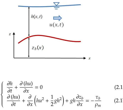
Figure 2.1: Basic nota-tion used to write the 1D, mono-phase model equa-tions              ∂h

∂t +

∂(hu)

∂x =0 (2.1a)

∂(hu)

∂t +

∂ ∂x

hu2+1 2gh

2₊_gh∂zb ∂x =−

τb

ρm (2.1b)

t indicates time, h the flow depth, u the mixture velocity, g the gravitational acceleration,zbthe bed elevation,τbthe shear stress

and ρm the (constant) mixture density. Assuming that ρm is known, the unknowns of the problem are three: h, u and τb. Since the system equations are only two, a further, typically al-gebraic equations is use to "close" the problem, expressingτbas a function of the other variables. A lot of different formulation of

τbare available in the literature.

This approach shows a high level of simplification and, for this reason, often is preferred to the two-phase approach. However, some of its assumptions appear quite debatable.

The mono-phase approach assumes necessarily that sediment concentration (and therefore density) is constant in space and time, although, in natural high-concentration flows, concentra-tion varies according to hydrodynamics.

Then, mono-phase models do not allow mass exchanges bet-ween mixture and bed, therefore neither erosion nor deposition processes can be described properly. The only variation of the bed elevation is considered during the stopping phase, assuming that the bed elevation increases by the flow depth.

(55)

2.1. Complexity and mathematical modelling

away.

For these reasons, the use of such models to simulate two-phase, cohesionless flows appears as an oversimplification, espe-cially if the flow moves over an erodible bed.

Current mono-phase models for mountain-flow simulations can be divided basically into two groups: Cellular-Automata-like models (hereafter CA-Cellular-Automata-like models) and Partial-Diff erential-Equations-based models (hereafter PDE-based models).

CA-like models are based, partially or totally, on di