Volume 9 - Article 5 | Pages 81–110

in the population sciences published by the Max Planck Institute for Demographic Research Konrad-Zuse Str. 1, D-18057 Rostock · GERMANY www.demographic-research.org

DEMOGRAPHIC RESEARCH

VOLUME 9, ARTICLE 5, PAGES 81-110

PUBLISHED 10 OCTOBER 2003

www.demographic-research.org/Volumes/Vol9/5/

DOI: 10.4054/DemRes.2003.9.5

Research Article

A system of model fertility schedules with

graphically intuitive parameters

Carl P. Schmertmann

1 Introduction 82

2 Description of fertility schedules by means of index ages

82

3 Mathematical definitions 84

3.1 The spline model 84

3.2 Linking the spline model to index ages 86

4 Fitting good data, Example #1: Comparison with Coale-Trussell

89

4.1 Data 89

4.2 Fitting procedure 89

4.3 Fitting results 91

4.4 Discussion 93

5 Fitting good data, Example #2: Patterns in contemporary Sweden

95

6 Fitting noisy data 97

7 Conclusion 103

8 Acknowledgements 103

Notes 104

References 106

Appendix A: Shape limitations of the CT model 108

Appendix B: Non-matrix calculation of spline coefficients

Research Article

A system of model fertility schedules

with graphically intuitive parameters

Carl P. Schmertmann 1

Abstract

I propose and examine a new family of models for age-specific fertility schedules, in which three index ages determine the schedule's shape. The new system is based on constrained quadratic splines. It has easily interpretable parameters, is flexible enough to fit a variety of "noiseless" schedules well, and is inflexible enough to avoid implausible estimates from noisy data. Across a set of over two hundred contemporary ASFR schedules, the new model fits a majority better, and in some cases much better, than the Coale-Trussell model.

When fit to a recent Swedish time series, model parameters exhibit simple, regular changes over time, suggesting utility in forecasting applications. In simulated small-sample data the new model produces plausible ASFR estimates, with errors similar to Coale-Trussell.

1 _{Center for Demography and Population Health. Florida State University. Tallahassee, FL}

1. Introduction

Parametric models have many important applications in demographic research. They are useful when creating hypothetical rate schedules in forecasting and projection exercises. They can serve to condense complex data into meaningful indices, in the manner of Coale and Trussell’s (1974) m index of fertility control. They are also essential for statistical estimation and smoothing when demographers have only partial or noisy data.

In this paper I examine a new family of parametric models for age-specific fertility rate (ASFR) schedules. In this family three index ages define the shape of the ASFR schedule. The new system satisfies several requirements for a good mathematical description of fertility patterns. It conforms to known regularities in ASFR schedules, has easily interpretable parameters, is flexible enough to fit a variety of “noiseless” schedules very well, and is inflexible enough to avoid producing highly implausible estimates from noisy data.

2. Description of fertility schedules by means of index ages

The model system that I propose describes the shape of the ASFR schedule in terms of the ages at which the schedule reaches certain characteristic points, specifically

", the youngest age at which fertility rises above zero,

P, the age at which fertility reaches its peak level, and

H, the youngest age above P at which fertility falls to half of its peak level.

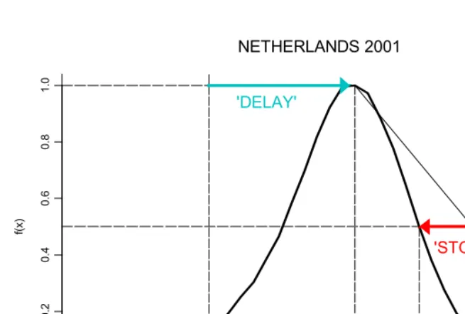
This approach builds model fertility schedules from easily visualized, geometric parameters measured in common units – namely “years”. Figure 1 illustrates with a period schedule of empirical 1fx values from the Netherlands in 2001 (Statistics

Netherlands 2003). The schedule is standardized so that the value at the mode is one, a convention that I will use frequently in this paper.

The Netherlands 2001 schedule reaches its peak at P.31.5 (the midpoint of the single-year age group “31") and falls to half of its peak level at H.36.6 (interpolated). These two ages are marked with solid squares in Figure 1. Given only the values of P

and H, together with the initial age ", most demographers could draw the shape of the ASFR schedule fairly accurately by hand.

Figure 1: Single-year ASFR schedule for Netherlands 2001, standardized with value at mode = 1.

schedule Nx at P=20, and very few empirical schedules have P < 20. The age difference

D = P – 20

can therefore serve as a useful index of the “delay” in achieving peak fertility. In the Netherlands 2001 schedule, D.11.5. Higher values of D suggest more delayed childbearing, perhaps due to later intercourse, later marriages, or to greater educational and employment opportunities for women.

On the right-hand side of the ASFR curve at ages x > P, demographers often use the degree of concavity of f(x) as an indicator of parity- or duration-specific fertility control. In the Coale-Trussell system this concavity is measured in terms of vertical

displacement, at ages above 20, from a standard schedule. It is equally informative, however, to measure the degree of concavity in terms of horizontal displacement. The arrow labeled “Stopping” in Figure 1 illustrates such an index of post-peak fertility control, defined mathematically as

age

f(

x)

10 20 30 40 50

0.

0

0

.2

0.

4

0

.6

0.

8

1

.0

NETHERLANDS 2001

'DELAY'

'STOPPING'

S = (P + 50)/2 - H

If fertility fell linearly from a peak at age P to zero at age 50 (straight diagonal line), it would reach the halfway point of descent at age (P+50)/2. The S index therefore indicates how many years earlier than that fertility actually reaches its halfway point. In the Netherlands 2001 schedule, S.4.2. High values of S correspond to greater concavity in the right-hand side of the ASFR schedule.

Note that on this scale S could be negative, indicating convexity in f(x) after its peak. For example, S= -5.2 in the Coale-Trussell Nx schedule. In addition, if P and H

both increase equally (similar to the general rightward drift in the ASFR schedule examined in Bongaarts and Feeney 1999), then a decreasing portion of the eventual fall toward zero fertility at the highest ages would be attributed to “stopping”.

S is empirically similar to the Coale-Trussell m index. Across the 3822 Coale-Trussell model schedules in Appendix A (discussed more fully in later sections) the correlation between S and m is +.82. In 226 contemporary empirical schedules (also discussed later) the correlation between estimated S and m is +.88.

3. Mathematical definitions

3.1. The spline model

The formal model used throughout this paper represents age-specific fertility rates between age " and an upper age $ as a piecewise quadratic spline function. There is a small literature on spline functions as fertility models. McNeil, Trussell, and Turner (1977) discussed using splines to smooth and interpolate fertility data. As an illustration, they used a quartic spline to model a continuous schedule f(x) that exactly matched a published set of fertility rates for five-year age groups. Hoem et al. (1981) found that cubic spline functions fit Danish fertility schedules from 1962-1971 far more accurately than other models, including Coale-Trussell. Gilks (1986) used cubic splines to model duration-specific effects of covariates on birth hazards.

The QS function used to build the new set of model fertility schedules in this paper is:

( ) ( )

f x ₌ R x_B (1)

where the shape function is a quadratic spline

4

2

0

( ) ,

( )

0 otherwise

k k

k

x t x

x G = >

B +

=

ì _{- £ £}

ï = í ïî

å

“knots” t0<t1<...<t4 fall in the interval between " and $ (in all models in this paper t0=", the lowest age of childbearing), and (x-tk)+/ MAX[0, x-tk]. For future reference, note that the QS function yields a closed-form expression for TFR:

4

3

0

( ) ( ) ( )

3 k k

k

R

TFR f x dx R x dx t

> >

= =

B G >

=

=

_ò

_ò

å

The f(x) function is continuous, with quadratic subsections joined at knot values. The slope of f is also continuous:

4

0

( ) ( ) 2 _k( _k) ,

k

f x RB x R G x t + = x >

=

¢ = ¢ =

å

In contrast, the second derivative is discontinuous, with discrete jumps at knot values:

[

]

4

0

( ) 2 _{k k} ,

k

f x R_j x R _q I x t _a x _b

=

¢¢ = ¢¢ =

å

where I[ ] is an indicator function equal to one if the condition in brackets is true and equal to zero otherwise.

t1 < x # t2, to 2R(20+21+22) over the interval after that, and so on. The slope of f is continuous, but a positive 2k indicates an increase in upward curvature (or a decrease in downward curvature) beginning at age tk. An initial parabola can then be bent into a variety of shapes over [",$] by selecting different sets of knots t and curvature shifts .

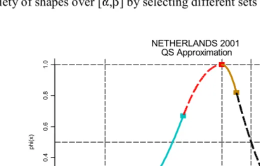
Figure 2: Quadratic Spline approximation to Netherlands 2001 schedule. Spline is assembled from five separate quadratic sections, as shown.

Figure 2 depicts an example that approximates the shape of the Netherlands 2001 schedule in Figure 1, using five distinct quadratic pieces and Equation (2) with

t = [ 15.6, 26.8, 32.4, 34.5, 42.9 ] = [+.00533, -.01609, -.03018 , +.05039, -.00840 ]

This quadratic spline function approximates the shape of the empirical schedule well, and with an appropriate choice of R, Equation (1) will serve as a good approximation to the period f(x) schedule.

3.2. Linking the spline model to index ages

The QS model is potentially useful for describing the shape of many fertility schedules, but it has thirteen parameters (R, ", $, t, ), and their meaning is somewhat opaque.

P

x

phi

(x

)

10 20 30 40 50

0.

0

0.

2

0.

4

0.

6

0.

8

1.

0

NETHERLANDS 2001 QS Approximation

Fortunately, it is possible to construct a spline model in which the three index ages [", P, H] uniquely determine the shape function N(x), and the multiplier R determines the level of fertility. The keys to reducing the number of parameters are (1) to determine knot positions from the index ages, and (2) to impose mathematical restrictions so that the spline function mimics common features of ASFR schedules.

Shape restrictions and knot placements are slightly arbitrary, and more than one set of assumptions could produce useful models. For the model system used in this paper, the specific assumptions for the shape function are:

1. Knot 0 is at the lowest age of fertility: t0 = "

2. Knot 1 is between the initial and peak ages of fertility (closer to peak if peak is late – Note 1):

t1 = (1-W)"+WP

W = min [ .75, .25 + .025(P-") ]

3. Knot 2 is at the peak age of fertility: t2 = P

4. Knot 3 is halfway between the peak and the halfway point of descent t3 = (P + H)/2

5. Childbearing ends at 50 (with minor adjustments for very steep or very flat schedules – Note 2):

(

)

(

)

(

)

(

)

(

)

(

)

1 3

1 1

3 3

50 if 50 3

if 50

3 if 3 50

H H P H H P

H H P H H P

H H P H H P

β

ì + − ≤ ≤ + −

ïï

= _í + − + − >

ï _{+ − + − <}

ïî

6. Knot 4 is halfway between the halfway point of descent and $: t4 = (H + $)/2

7-9. Fertility at ages P, H, and $ equals 1, 1/2, and 0, respectively (arbitrary units) N(P) = 1 N(H) = 0.5 N($) = 0

For a wide range of reasonable values of index ages [",P,H], these restrictions imply a unique shape function N(x):

, ,P H restrictions t, ( )x

= + Þ G Þ B

Note that spline knots and coefficients are not particularly important in their own right; they are merely an intermediate step linking the age parameters [",P,H] to the shape function N. Knot values t are given directly by assumptions 1-6. The spline coefficients must solve the following system of linear equations based on 7-11:

2 2

1 ₀

2 2 2 2

1

1 2 3

2 2 2 2 2

2

1 2 3 4

3 1

4

1 2 3 4

0 0 0 ₁

0.5 0

0 0

2 2 0 0 0

0

2 2 2 2 2

P P t

H H t H t H t

t t t t

P P t

t t t t

a _q

q a

q

b a b b b b

q a

q

b a b b b b

é _{- -} ù_{é ù é ù}

ê _{ú ê ú ê ú}

ê - - - - ú_{ê ú ê ú}

ê _{ú ê ú ê ú=}

ê - - - ú_{ê ú ê ú}

ê _{- - ú ê ú ê ú}

ê _{ú ê ú ê ú}

ê - - - úë û ë û

ë û

(6)

or more compactly

k

G =

A (7)

For demographically plausible values [",P,H], A is non-singular, and the spline coefficients are

G = _{= A}- ₍₈₎

These coefficients are then substituted into Equations (2) and (3)

Although this system of equations looks complicated, it is trivially easy to solve with most contemporary software. For example, the spreadsheet in File I accompanying this paper makes use of matrix formulas to solve for the spline coefficients, and on a desktop personal computer (circa 2002) the computations and curve drawing appear to be virtually instantaneous after one enters the indices. Without software that operates directly on matrices and vectors, it remains possible to calculate spline coefficients rapidly on a computer; the necessary formulas are less elegant, but simple to program (see Appendix B).

File I, manipulate the parameters with the controls provided, and examine the resulting changes in the ASFR schedule. Readers familiar with spreadsheet formulas may also examine the calculations in detail.

4. Fitting good data, Example #1: Comparison with Coale-Trussell

4.1. Data

In order to test the utility of the new family of spline-based models, I fit both the QS model and the single-year CT model to each of a set of 226 national and area fertility schedules, from the U.S. Census Bureau’s International Data Base (IDB) (US Census Bureau 2002. See Note 3). A disadvantage of these data is that they are for five-year, rather than single-year, age groups. However, it is important to test the models across a very wide variety of observed ASFR schedules, and I know of no similarly comprehensive set of single-year-specific fertility rates. On balance, I believe that the breadth of the IDB data outweighs the disadvantages of age aggregation (Notes 4, 5, 6).

4.2. Fitting procedure

The CT model uses three shape parameters (a0, k, m) and a level parameter (TFR) to

generate single-year age-specific fertility rates, as follows. The first three parameters determine a shape function:

1 2

0

1

0 2

( ) ( | , ) exp( )

x CT

x x

a

x g a a k da N m v

B

+

é ù

ê ú

+ =

ê ú

ë

ò

(9)

where Nx and vx are the predefined constants for x=12...49 given in Coale and Trussell

(1974; see Note 7), and

0 0 0

.19465 .174 .2881

( | , ) exp 6.06 exp 6.06

g a a k a a k a a k

k k k

ì- é - ùü

æ ö ïæ ö æ ö ï

=_{ç ÷ íç ÷} - - - _{êç ÷} - - _úý

is a version of the Coale-McNeil (1972) nuptiality model with varying location (a0) and scale (k). The level of fertility is set by specifying a TFR for ages 15-49 and multiplying

N(x) values by an appropriate constant:

49

1 1 1

2 2

2

15

ˆ (CT ) CT( ) CT( )

a

f x TFR B x B a

=

+ = × +

å

Single-year rates are then aggregated into standard five-year groups using the formula

14 5

1 2 10 5

1

ˆ _{ˆ ( ) 1...7}

5 i

CT CT

i

x i

f + f x i

= +

=

å

The QS model uses index ages [",P,H] to generate spline knots and coefficients (t, ) as described above, with the shape of the fertility schedule defined by

4

2

0

( ) ( )

QS

k k

k

x x t

B G +

=

=

å

With max[N]=1 by construction, the level parameter R represents max[f(x)], and

1 1

2 2

ˆ (QS ) QS( )

f x+ =RB x+ (14)

Equation (3) contains a closed-form expression for the TFR.

For each observed fertility schedule [f15-19...f45-49], I fit both the CT and QS models by selecting shape and level parameters that minimized the sum of squared errors (Note 8):

7 2

1

ˆ i i i

SSE f f

=

=

å

where fi is the observed rate for age group i from the Census data base. I also use a measure of relative error in the shape function:

ˆ

100 _{i i i}

i i

RE = æ_ç f -f ö æ_{÷ ç} f ö_÷

RE measures the ratio of absolute prediction errors to TFR; Coale and Trussell (1978:204) advocated its use as a goodness-of-fit measure when interpolating single-year rates from observations on five-single-year age groups.

4.3. Fitting results

File II illustrates the complete set of 226 schedules, together with the corresponding CT fits (red squares) and QS fits (blue lines). The relative errors for the QS and CT models appear at the top of the graph for each schedule. In addition to this graphical presentation, the complete set of observed fertility rates, parameter estimates, and REs is included in

File III

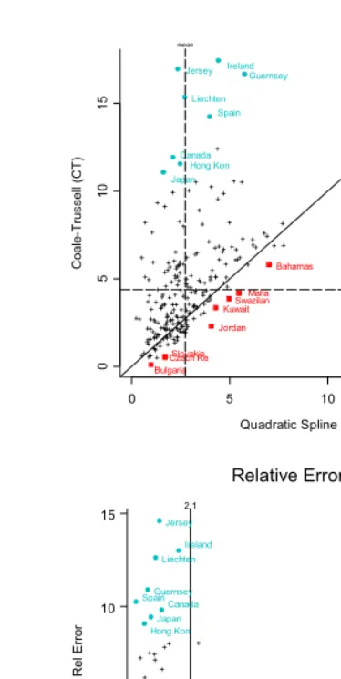
Table 1 contains summary information on the OLS fits for the 226 schedules, and Figure 3 plots the CT relative error against the QS relative error for each schedule.

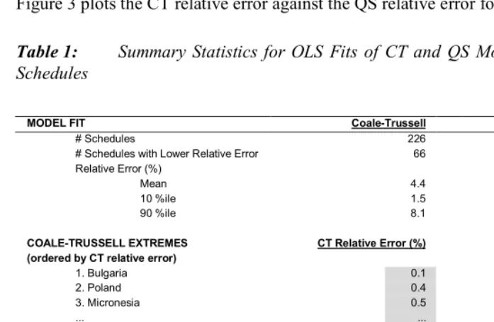
Table 1: Summary Statistics for OLS Fits of CT and QS Models to International Schedules

MODEL FIT Coale-Trussell Quadratic Spline

# Schedules 226 226

# Schedules with Lower Relative Error 66 160

Relative Error (%)

Mean 4.4 2.7

10 %ile 1.5 1.1

90 %ile 8.1 4.8

COALE-TRUSSELL EXTREMES (ordered by CT relative error)

CT Relative Error (%) QS Relative Error (%)

1. Bulgaria 0.1 1.0

2. Poland 0.4 1.2

3. Micronesia 0.5 0.8

... ... ...

224. Guernsey 16.7 2.6

225. Jersey 16.9 4.5

226. Ireland 17.4 1.4

QUADRATIC SPLINE EXTREMES (ordered by QS relative error)

CT Relative Error (%) QS Relative Error (%)

1. Romania 0.6 0.5

2. Norway 5.8 0.6

3. Switzerland 9.1 0.6

... ... ...

224. Iraq 7.5 7.6

225. Somalia 8.1 7.6

Figure 3: Relative errors of Coale-Trussell and Quadratic Spline model fits to observed five-year schedules. Top panel depicts relative percentage errors for each schedule. Bottom panel depicts difference in relative errors (CT minus QS) as a function of total fertility. Schedules for which QS model has lower relative error fall above the 45-degree line in top panel and above horizontal “0" line in the bottom panel. Schedules with biggest relative error differences in favor of QS or CT are labeled and marked with blue dots or red squares, respectively.

Quadratic Spline (QS)

C oal e-T rus se ll ( C T )

0 5 10 15

05 10 15 ++ + + + + + + + + + + + + + + + + + + + + + + + + + + + + + + + + + + + + + + + + + + + ++++ + + + + + + + + + + + + + + + + + + + + + + + + + + + + + + + + + + + + + + + + + + + + + + + + + + + + + + + + + + + + + + + + + + + + + + + + ++++ + + + +++ + + + + + + + + + + + + + + + + + + ++ + + + + + ++ + + + + + + + + + + + + + + + + + + + + + ++ + + + +++ + + + + + + + + + + ++ + + + + +++++ + +

Jersey Ireland Liechten Guernsey Spain Canada Japan Hong Kon Jordan Malta Bahamas Slovakia Czech Re Swazilan Kuwait Bulgaria mean mean TFR C T -Q S R el E rro r + + + + + + + + + + + + + + + + + + + + + + + + + + + + + + + + + + + + + + + + + + + + + + + + ++ + + + + +₊ + + + + + + + + + + + + + + + + + + + + + + + + + + + + + + + + + + + + + + + + + + + + + + + + ++ + + + + + +++ + + + ++ + + + + ++ ++ + + + + + + + + ++ + + + + ++ +₊+ + ++ ++ + ++ +++++ +++₊₊+ + ++ + +++ + + + + + + ++ + + + + + + + ++ +++ + + + +++ + ++ + ++ + + ++ + +

1 2 3 4 5 6 7

0 5 10

15 _Jersey 2.1

Ireland Liechten Guernsey Spain _Canada

Japan Hong Kon

Jordan Malta Bahamas Slovakia

Czech Re Swazilan Kuwait

Bulgaria

Because readers may examine the fits at any desired level of detail in Files II and III, I provide only an overview here. Some broad conclusions from fitting the 226 schedules in the IDB are:

1. CT and QS fits are very similar for most schedules.

2. Both models fit most empirical schedules well (e.g., for 150 of 226 schedules, both have relative errors < 5%). These good fits are comforting, but not especially surprising, because both models fit seven target values using four parameters (3 shape, 1 level).

3. The QS model fits the majority of schedules more accurately (160 of 226)

4. There are no schedules in the IDB for which the CT model fits well and the QS model fits badly. This is evident in both panels of Figure 3.

5. In contrast, there are schedules for which the CT model fits badly and the QS model fits well. The QS model has notably lower relative errors than CT for schedules with low TFRs, delayed childbearing, high modal ages, and steep right-hand sides. Examples include many Western European countries (e.g, Spain, Netherlands, Ireland, and Liechtenstein) and other high-income countries such as Canada and Australia. The right-hand panel of Figure 3 illustrates this point by plotting TFR against the difference

RECT-REQS: note that schedules for which the CT model has a much larger relative errors are primarily those with below-replacement levels of TFR.

4.4. Discussion

Fitting models to the IDB schedules demonstrates the utility of the QS model as a tool for summarizing and interpolating fertility schedules. The QS model fits a wide variety of schedules well.

maternal ages. As a consequence, increases in m make the right-hand side of the schedule steeper and lower the modal age (P).

This CT tradeoff between the peak age P and the rate of descent after P can lead to awkward compromises that fail to fit either side of the ASFR schedule well. As an example, Figure 4 once again depicts the Netherlands 2001 single-year schedule (from Figure 1, approximated with a QS model in Figure 2), this time including the best CT approximation (in a least-squares sense, as in Hoem et al. 1981). The dashed line in the figure represents the best-fitting member of the CT family, specifically (a0,k,m)=(21.4, 2.01, 3.41). The high values of a0 and k (representing late starts and slow marriage rates, respectively) act to push the peak age to the right. The high level of

m (high control) makes fertility fall sharply over post-peak ages. However, neither the peak nor the right-hand slope comes out quite right. Raising a0 and k further to push the peak rightward would worsen the fit too much at low ages. On the other hand, raising

m further to increase post-peak steepness would push the mode leftward and

(paradoxically) worsen the fit at high ages. This particular schedule represents the best compromise to be found, but it is not a particularly good representation of the Netherlands schedule.

Figure 4: Best (least squares) fit for Coale-Trussell model to Netherlands 2001 single-year schedule.

age

phi

(x

)

20 30 40 50

0.0 0.25 0.50 0.75 1.00

NETHERLANDS 2001

Appendix A reports more fully on lacunae in CT schedules’ shapes. The central point in this discussion is not criticism of the CT model, which was not designed to describe contemporary schedules with very low fertility. Instead, the point is that the

QS model system is flexible enough to describe the geometry of “new” ASFR

schedules such as those in Western Europe. As such, the QS model could be a useful framework for projections, forecasts, and explorations of fertility in developed, as well as the developing, countries. The next section provides an example.

5. Fitting good data, Example #2: Patterns in contemporary Sweden

Parametric models are useful for summarizing patterns in high-dimensional data. In this section I briefly illustrate use of the QS model for this purpose, by fitting models to contemporary Swedish fertility schedules and examining parameter changes over time. Kohler and Philipov (2001) analyzed 1975-1996 Swedish period fertility trends thoroughly. I use their data (Note 9).

For each of the 22 years, I fit a QS schedule to the observed single-year rates for Sweden by selecting [",P,H] to minimize the sum of squared errors

2 1

1 2

ˆ (QS ) ( )

x x

f x f t

é _{+ -} ù

ë û

å

The QS model fits all 22 years well. Relative errors range from a low of 2.4% in 1979 to a high of 4.4% in 1995. In the later years of the time series the QS model tends to overestimate fertility rates at the maternal ages 40+, but that problem is small. The complete set of fits, including plots of time series for estimated !, P, and H, is contained in a spreadsheet in File IV. I encourage the reader to open the spreadsheet, manipulate the controls to change the year, and examine the fits and parameter values in detail.

QS model parameters exhibit simple, regular patterns of change over the 22 years. Specifically, both P and H increase nearly linearly, while ! remains approximately constant. P rises steadily from 25.3 in 1975 to 29.2 in 1996 (the average change is +.18/year), and H rises in near lock-step, from 31.7 to 35.1 (+.16/year). Estimates of initial age ! change more irregularly, and on a smaller scale: ! rises in fits and starts from 14.1 to 15.0 over 1975-1996 (+.04/year).

TFR (Bongaarts and Feeney 1998). Kohler and Philipov stressed that changes in Sweden matched one important mathematical assumption of the BF formula fairly well (mean age of childbearing exhibited approximately linear increase), but did not match another main BF assumption (the variance of the age of childbearing increased, rather than staying constant as assumed in BF).

Parameter changes in the QS model provide a parsimonious explanation that reconciles linear changes with increasing variance. Taken together, the nearly constant

" with linearly increasing P and H suggest that the peak and the right-hand side of the

f(x) schedule were sliding rightward at a fairly constant rate (as in BF), but that variance increased because the left-hand side of the ASFR schedule was being stretched horizontally as " rose more slowly than P (contrary to BF) and P-increased.

The changes in estimated QS parameters are very regular, making them useful for studying behavior. Figure 5 depicts the time series of the estimated D and S indices (described previously) for Sweden over the period under study. Childbearing was increasingly delayed, pushing D up steadily as the age of peak fertility rose. As measured by S, post-peak fertility rates exhibited decreasing concavity, suggesting small, steady decreases in fertility control at higher ages (Note 10).

Figure 5: Time trends in estimated D and S values for Sweden 1975-1996.

Calendar Year

Y

ear

s

Trends in QS Parameters Sweden 1975-1996

1975 1980 1985 1990 1995

4 5 6 7 8 9 10

'Delay'

Most importantly for the purposes of this paper, the simple time series patterns in Figure 5 demonstrate the QS model’s ability to capture and highlight meaningful mathematical regularities in empirical fertility schedules. They also signal the potential utility of using times series for D(t) and S(t) as a language in which to express projections and forecasts about future changes in fertility’s “tempo”.

6. Fitting noisy data

Data are frequently less abundant than in the cases studied so far. Model schedules are often used to estimate fertility from small samples or from other data subject to random errors. In these circumstances it is important that models not be too flexible, in the sense that coincidental variations in a sample should not be overinterpreted as representing real features of the fertility regime. In loose statistical terms, we would like models with enough degrees of freedom to produce a variety of shapes and levels for estimated fertility schedules in response to reliable evidence, but also with enough mathematical rigidity to remain fairly stable in response to sampling noise. These are of course competing goals, and much of the art of statistical modeling consists of finding approaches that balance flexibility (low bias) against stability (low variance).

I investigated the flexibility and stability of the QS model by running a series of Monte Carlo experiments in which I estimate single-year ASFR schedules from small samples. In each sample I assume that the true single-year age-specific fertility rates for ages 15-49 belong to one of five schedules:

a. the CT fit to the El Salvador schedule from the US Census International data base [ESA02], taken from File III: (TFR,a0,k,m)=(3.29, 12.3, .52, .81)

b. 1999 period fertility for the Czech Republic [CZE99], from the Czech POPIN website(Czech Republic 2002)

c. 1971-75 period fertility for South Korea [KOR71], from Coale, John, and Richards (1985)

d. 1996 period fertility for Sweden [SWE96], from Kohler and Philipov (2001)

I selected these schedules because of their differences in shape and level, as illustrated in Figure 6.

Figure 6: Single-year period ASFR schedules (1000 1fx) for El Salvador 2002,

Czech Republic 1999, South Korea 1971, Sweden 1996, and Australia 2000. El Salvador schedule is a Coale-Trussell model fit to five-year data; other schedules are empirical observations.

The five schedules a-e are ordered in terms of peak ages of fertility, which are 22, 25, 26, 29, and 30, respectively. From results with IDB schedules in Section 3, we would expect that the QS model would fit all five of these “true” schedules well, while the CT model might have difficulty fitting the Swedish and Australian curves. At this point we do not know whether the extra flexibility of the QS model comes with a high price in terms of sampling variability; the purpose of the Monte Carlo sampling experiment is mainly to investigate these bias-variance tradeoffs.

For each of the five schedules {fx} I tried three sample sizes, consisting of N=10,

100, or 1000 women per single-year age group (Note 11). There are therefore 15 basic experiments, one for each combination of [{fx},N]. For each of these 15 experiments the

computer program generated 200 Monte Carlo samples of births {Bxs}, using

15 25 35 45

0 50 100 150 200 250 300

SWE96 KOR71

CZE99 ESA02

~ , , 15...49 1...200

xs x

B Binomial N p= f x= s=

The computer program then chose the QS parameters [R,",P,H] that minimized the sum of squared errors for each sample s=1...200:

2

ˆ

( )

s x xs

x

Q =

å

and calculated the mean squared error across both ages and samples:

200 49 2

1 15

1 _ˆ

35 200 xs x s x

MSE f f

= =

=

-×

å å

If we denote the average fitted rate at age x by

200

1

1 _ˆ

200

x xs

s

f f

=

=

å

then MSE may be further decomposed into squared bias and variance terms:

49 2 200 49 2

15 1 15

1 1 _ˆ

35 x x 35 200 xs x

x s x

MSE f f f f

= = =

é ù

é ù

= _ê - _ú + _ê - _ú

ë û × ë û

å

å å

or, in more intuitive notation:

2 2 2

RMSE = BIAS + STDEV (22)

where RMSE represents the root mean squared error, BIAS represents the estimated effects of systematic fitting errors (i.e., the inability of the model to fit the “true” ASFR schedule), and STDEV represents the estimated effects of sampling variability (i.e., the average amount of noise in a typical 1fx estimate). I also fit the CT model to the same

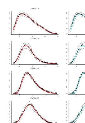
Figure 7: Monte Carlo sample results. Left-hand panels are for CT fits; right-hand

panels for QS fits. Points (+) are “true” f(x) schedules; solid lines are

best fits in “noiseless” samples (N="); dashed lines are 10th _{and 90}th

percentiles of fits when N=100 women are sampled at each age.

ESA02 / CT

20 30 40 50

0 50 100 150 200 ++ + +++++++++++++ +++ ++++₊₊₊ +++++++++

ESA02 / QS

20 30 40 50

0 50 100 150 200 ++ + +++++++++++++ +++ ++++₊₊₊ +++++++++

CZE99 / CT

20 30 40 50

0 204 0 608 0 10 0 +++ ++ ++ +++ ++ ++ +₊ ++ +++ ++++++++++++++

CZE99 / QS

20 30 40 50

0 204 0 608 0 10 0 +++ ++ ++ +++ ++ ++ +₊ ++ +++ ++++++++++++++

KOR71 / CT

20 30 40 50

0 100 200 300 +++++ ++ + ++ +++ ++₊ + ++ ++ +++++_+++++++++

KOR71 / QS

20 30 40 50

0 100 200 300 +++++ ++ + ++ +++ ++₊ + ++ ++ +++++_+++++++++

SWE96 / CT

20 30 40 50

0 20 40 60 80 100 120 140 +++++ +++ ++ +++++++₊ +₊ ++ ++ +++++++++++

SWE96 / QS

20 30 40 50

0 20 40 60 80 100 120 140 +++++ +++ ++ +++++++₊ +₊ ++ ++ +++++++++++

AUS00 / CT

20 30 40 50

0 204 06 08 0 10 0 12 0 14 0 ++++ ++++ ++++ ++++++₊ +₊ + ++ +++_++++++++

AUS00 / QS

20 30 40 50

Figure 7 displays some of the Monte Carlo results from small-sample fitting. In the 5x2 grid of panels, each row corresponds to one of the five “true” schedules, which are depicted with + signs. The first column of panels (with red lines) represents Coale-Trussell fits, and the second column (blue lines) represents Quadratic Spline fits. Solid lines in each panel show the best model fit to the true schedule (i.e., the limiting sample fit as N64), and dashed lines show the 10th _{and 90}th _{percentiles of sample fits when}

N=100.

The fits to the true schedules provide information about the models’ flexibility/bias. Consistent with earlier results, the QS model is able to fit all five schedules accurately, but the CT model exhibits small biases for SWE96 and fairly large biases for the AUS00 schedule. The CT model’s lack of fit for AUS00 (bottom left panel) is very similar to that in the Netherlands schedule in Figure 4: rates are too low at young ages, the peak is too early, and the right-hand side is too flat.

Distances between the lower and upper dashed lines provide information about the models’ sensitivity/variance. Figure 7 shows that pointwise 80% confidence bands for the CT and QS models are quite similar in the N=100 case. Bands for N=10 and

N=1000 are not shown, but the conclusion is the same: CT and QS estimates exhibit similar levels of variability across the Monte Carlo samples at all sample sizes.

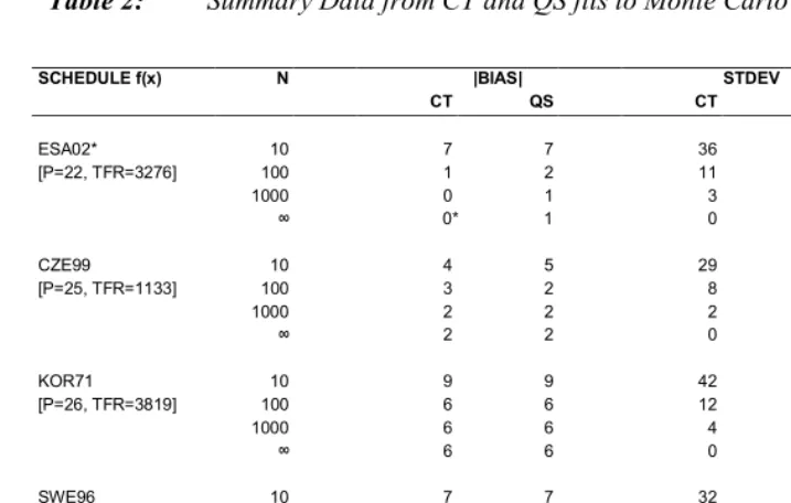
Table 2 provides a more complete summary of the Monte Carlo experiments. It includes information from N=10 and N=100 experiments, and it reports |BIAS|, STDEV, and RMSE measures (as defined in Equation 22) across the 200 samples for each [{fx},N] combination. Data in Table 2 show that the CT and QS models have similar

levels of small-sample variability. In very small samples the QS model may be more susceptible to sampling noise, but only slightly. Both models converge rapidly in the direction of the true {fx} as sample sizes increase, but for schedules with late peaks,

Table 2: Summary Data from CT and QS fits to Monte Carlo Samples

SCHEDULE f(x) N |BIAS| STDEV RMSE

CT QS CT QS CT QS

ESA02* 10 7 7 36 38 37 39

[P=22, TFR=3276] 100 1 2 11 11 11 11

1000 0 1 3 3 3 4

∞ 0* 1 0 0 0* 1

CZE99 10 4 5 29 30 29 31

[P=25, TFR=1133] 100 3 2 8 8 8 8

1000 2 2 2 2 3 3

∞ 2 2 0 0 2 2

KOR71 10 9 9 42 43 43 44

[P=26, TFR=3819] 100 6 6 12 12 13 13

1000 6 6 4 4 7 7

∞ 6 6 0 0 6 6

SWE96 10 7 7 32 33 33 34

[P=29, TFR=1598] 100 4 2 8 9 9 10

1000 4 2 2 3 4 3

∞ 4 2 0 0 4 2

AUS00 10 10 7 33 32 35 33

[P=30, TFR=1749] 100 9 3 9 9 13 9

1000 10 3 3 3 10 4

∞ 10 3 0 0 10 3

Note:

* The assumed “true” schedule for ESA02 is the Coale-Trussell fit to five-year data for El Salvador from Section 4. By construction the CT model will fit this schedule perfectly and the limiting value of CT bias is zero.

7. Conclusion

The QS model system proposed in this paper includes a wide variety of shapes for ASFR schedules. This includes some schedules (mainly from contemporary Western Europe) for which the most familiar demographic model, Coale-Trussell, cannot fit well. Because QS parameters [, P, H] are ages at which the ASFR schedule has certain characteristics, back-and-forth translation between model parameters and shape functions becomes simple and intuitive. The QS model also produces a continuous ASFR function f(x) and closed-form expressions for quantities such as TFR, features which may be analytically convenient.

QS fits to recent Swedish time series find simple, easily interpretable patterns that describe the changing timing of fertility very well. This suggests that the QS model could be a good tool for simulation and projection exercises, particularly for scenarios which include changes in the “tempo” of fertility.

Small-sample Monte Carlo experiments demonstrate that the QS model is not oversensitive to sampling noise (a serious problem for some spline-based models), and that it produces reasonable ASFR estimates even in very small samples. Average errors are very similar to those obtained with the Coale-Trussell model.

Splines are an extraordinarily flexible family of continuous functions. They are often too flexible for demographic purposes, because a specification such as Equation (2) often includes not only a wide array of plausible functional forms for a particular application, but many implausible forms as well. One main idea behind the QS model is to “tame” spline functions by insisting that they have certain features (peak at P, zero value and zero slope at , etc.), and by limiting knot values and parameters to subspaces that correspond to “good” demographic models. This taming process reduces the number of parameters necessary to describe a function. Another main idea behind the QS model is that for demographic models the reduced parameter set can consist of ages

at which the function has certain features. The combination of constrained splines and age-index parameters produces a family of good demographic models with easily understood arguments. Demographers could use these ideas in many other models and applications.

8. Acknowledgements

Notes

1. Knot value t1 always falls between and P. Condition 2 places t1 exactly halfway

between and P if P-=10, closer to P if the interval between initial and peak fertility is more than 10 years, and closer to if the interval is less than 10 years. I had initially set t1=(+P)/2 for all parameter values, but examination of a small

number of empirical 1fx schedules (different from those used in the Monte Carlo

study in Section 6) suggested that the inflection point of the ASFR schedule tends to be at higher ages when P is high, and vice-versa. The changing value of W in condition 2 allows the left-hand (pre-peak) side of the fertility schedule to match the empirical observations more closely, by becoming more concave for schedules with wider left-hand sides and more convex when the left-hand side is narrower. 2. Under this definition the maximum age of childbearing equals 50 for most sets of

parameters. However, to ensure a non-positive slope for the ASFR schedule at all ages above P, adjustments to become necessary when the “half life” of fertility (H-P) is either very small or very large (corresponding to very steep or very flat post-peak schedules, respectively). Analysis shows that post-peak slopes are non

positive if H+(H-P)/C#H+C(H-P), where C=(3+17)/2.3.5616

.

falls within even narrower bounds.

3. The data consist of 226 sets of seven period fertility rates [f15-19...f45-49], each from

the latest available year for each country or area.(From the web site I selected: “Table 28", “All Countries”, “Latest Available Year”. In all cases the “latest available year” was labeled “2002".)

4. I corresponded with the US Census Bureau to verify that the IDB schedules were not themselves constructed or adjusted with spline or Coale-Trussell models. They are not. Peter Johnson (personal communication) indicates that IDB reporting procedures vary for different schedules, and that in some cases the Census Bureau uses demographic models (although not splines or CT models) to adjust reported fertility levels. However, the shapes of the IDB schedules are unaffected by these procedures.

5. There are several ways of fitting the CT and QS models to observations from five-year age groups. Coale and Trussell (1974) present both a complete version of their model, for single-year age groups, and an abridged version for five-year groups. In the QS model fertility rates are a continuous function of exact age, and there are closed-form expressions (not shown in the text) for nfx values. For purposes of

comparison I opted to use “single-year” versions of both models, in which 5fx is

approximated by [f(x+0.5) + ... + f(x+4.5)]/5.

6. With data in five-year groups beginning at age 15, both the CT and QS models may use implausibly low (or even negative) values of the initial age parameter (a0 or ,

respectively) to fit schedules with high values of 5f15. In the fits reported here I

have constrained initial age parameters in both models to be positive, but not necessarily >10. The results include several schedules (e.g. Bangladesh, Cuba, Grenada) in which the initial age parameter helps the fit at ages 15+, but should not be interpreted as anything other than an arbitrary mathematical value. With single-year data this problem tends to disappear. I thank students in Joe Potter’s Spring 2003 Demographic Methods class at the University of Texas for alerting me to this detail.

7. Although the text of Coale and Trussell (1974) contains N and v values for five-year age groups only, single-five-year values are available from the Fortran code in their Appendix A (p. 202).

8. Minimizing this particular SSE criterion is one of many possible fitting procedures. For a brief discussion of alternative objective functions, and a pragmatic argument for using unweighted least squares, see Hoem et al. (1981:231-232).

9. Data for Sweden are 1975-1996 period schedules of single-year ASFRs (all parities combined). These are originally from the Eurostat New Cronos data base (1998), as cited in Kohler and Philipov (2001), and are available on Kohler’s web site (Kohler 2003).

10. Coale-Trussell models fit to the Swedish time series (not shown) have less regular patterns. However, estimated control m decreases almost linearly from a high of 3.7 in 1980 to a low of 3.0 in 1995.

References

J. Bongaarts and G. Feeney, 1998. "On the quantum and tempo of fertility," Population and Development Review (24)2:271–291.

H. Booth, 1984. “Transforming Gompertz's Function for Fertility Analysis: The Development of a Standard for the Relational Gompertz Function”. Population

Studies 38(3):495-506.

A.J. Coale, A.M. John, and T. Richards, 1985. “Calculation of Age-Specific Fertility Schedules from Tabulations of Parity in Two Censuses”. Demography

22(4):611-623.

A.J. Coale and D.R. McNeil, 1972. “The Distribution by Age of the Frequency of First Marriage in a Female Cohort”. Journal of the American Statistical Association

67(340):743-749.

A.J. Coale and T.J. Trussell, 1974. “Model Fertility Schedules: Variations in the Age Structure of Childbearing in Human Populations”. Population Index 40(2):185-258.

A.J. Coale and T.J. Trussell, 1978. “Technical Note: Finding the Two Parameters that Specify a Model Schedule of Marital Fertility”. Population Index 44(2):203-213. Czech Republic, 2002. Population Information (POPIN) website. Fertility rates downloaded 18 July 2002 from URL http://popin.natur.cuni.cz/html2/index.php? item=3.6 .

Eurostat, 1998. New Cronos Database: Population and Social Conditions. Brussels: Eurostat.

W.R. Gilks, 1986. “The Relationship between Birth History and Current Fertility in Developing Countries”. Population Studies 40(3):437-455.

J.M. Hoem, D. Madsen, J.L. Nielsen, E-M Ohlsen, H.O. Hansen, and B. Rennermalm, 1981. “Experiments in Modelling Recent Danish Fertility Curves”. Demography

18(2):231-244.

H-P Kohler, 2003. University of Pennsylvania web site. Downloaded 15 May 2003 from URL http://www.ssc.upenn.edu/~hpkohler/data-and-programs/bfvariance /se-nfx-all.txt.

D.R. McNeil, T.J. Trussell, and J.C. Turner, 1977. “Spline Interpolation of Demographic Data”. Demography 14(2):245-252.

Statistics Netherlands. 2003. Download 15 May 2003 from URL http://www.cbs.nl/StatWeb.

Appendix A: Shape limitations of the CT model

In order to examine the range of possible shapes inherent in the CT model system, I computed f(x) schedules over a grid of 13x14x21=3822 (a0,k,m) values defined by

(a0, k, m) 0 {8, 9, ..., 20} x {0.1, 0.4, 0.7, ..., 4.0} x {0, 0.2, 0.4, ..., 4.0}

and recorded the modal age P and halfway point of descent H for each schedule. A CT schedule consists of a vector of 38 rates [f12, f13, ...,f49] for single- year age groups, so

there is some natural ambiguity about exact-age values of P and H. For the crude purposes of the table below, I call P the integer age corresponding to the highest of the 39 rates in a schedule, and H the lowest integer age x for which x > P and f(x)< f(P)/2.

Appendix Table A1 shows the distribution of (P,H) combinations across the 3822 schedules. Each cell corresponds to a particular (P,H) combination, and therefore to a particular “shape” for the right-hand side of the ASFR schedule. Cells marked with dashes are logically impossible. Cells for other combinations contain the number of schedules with that particular combination of P and H. The focus is on the right-hand side of the fertility schedule. I omit other details for the sake of brevity.

The main finding from this analysis is that the CT family does not include schedules with rapid drops after peak fertility is reached, and that this is particularly true for schedules with peak ages in the low- to mid-30s. Such schedules have small values of H-P and would fall near the main diagonal in the table. Shaded cells represent logically possible (P,H) combinations for which there were no corresponding CT model schedules, and they tend to lie along this diagonal.

Appendix Table A1:

Number of schedules with given (P,H) values out of 3822 CT models (a0,k,m) = {8.9,…,20} x {0.1, 0.4, …,4.0} x {0, 0.2, …, 4.0}

Halfway Point of Descent (H)

<25 25 26 27 28 29 30 31 32 33 34 35 36 37 38 39 40 41 42 43 44 45

P

19 0 41 38 17 16 16 7 0 0 0 0 0 0 0 0 0 0 0 0 0 0 0

20 0 20 50 47 28 18 16 17 13 2 13 1 12 1 0 12 0 9 0 0 0 0

21 0 0 7 26 32 17 9 7 4 5 3 2 2 2 0 3 0 5 0 0 0 0

22 0 0 0 9 37 70 44 16 8 5 3 2 3 2 2 2 1 2 0 0 0 0

23 0 0 0 0 5 30 110 104 33 12 7 4 3 3 3 1 3 2 0 0 0 0

24 -- 0 0 0 0 5 22 46 47 20 7 4 4 1 2 1 2 1 0 0 0 0

25 -- -- 0 0 0 0 11 39 62 40 20 6 5 4 1 4 2 4 0 0 0 0

26 -- -- -- 0 0 0 0 18 90 120 83 57 33 21 9 6 3 6 0 0 0 0

27 -- -- -- -- 0 0 0 0 8 31 43 32 26 20 13 7 6 3 1 0 0 0

28 -- -- -- -- -- 0 0 0 0 13 51 67 84 64 53 40 16 7 2 0 0 0

29 -- -- -- -- -- -- 0 0 0 0 0 4 24 42 61 78 76 39 5 0 0 0

30 -- -- -- -- -- -- -- 0 0 0 0 0 0 0 4 22 47 68 13 0 0 0

31 -- -- -- -- -- -- -- -- 0 0 0 0 0 0 0 2 19 55 28 0 0 0

32 -- -- -- -- -- -- -- -- -- 0 0 0 0 0 0 0 1 46 80 0 0 0

33 -- -- -- -- -- -- -- -- -- -- 0 0 0 0 0 0 0 3 60 12 0 0

34 -- -- -- -- -- -- -- -- -- -- -- 0 0 0 0 0 0 0 71 43 0 0

35 -- -- -- -- -- -- -- -- -- -- -- -- 0 0 0 0 0 0 12 111 0 0

36 -- -- -- -- -- -- -- -- -- -- -- -- -- 0 0 0 0 0 0 93 0 0

37 -- -- -- -- -- -- -- -- -- -- -- -- -- -- 0 0 0 0 0 61 45 0

38 -- -- -- -- -- -- -- -- -- -- -- -- -- -- -- 0 0 0 0 0 109 0

Appendix B: Non-matrix calculation of spline coefficients

Calculating the spline parameters for the ASFR schedule is more awkward without matrix functions, but it is feasible. The derivation has two distinct steps, for parameters affecting the curve to the left and right of the peak, respectively.

The knots t0...t4 are defined as in the text. Parameters for the left-hand part of the

curve can be calculated from this sequence:

[

]

0 2 1

1

.75,.25 .025( )

1

W MIN P

W W P

G

= G G

=

-= + - = =

-Spline coefficients for the right-hand side can be calculated via a set of intermediate variables:

2 2 2

2 3 4

2 3 4

2 2

1 0 1 1

2 2

2 0 1 1

3 0 1 1

,

, ,

2 , 2 , 2

0.5

0

0 2 2

A B

C D E

F G H

A D H A E G C B H F B E

Z H t Z H t

Z t Z t Z t

Z t Z t Z t

Z H H t

Z t

Z t

DENOM Z Z Z Z Z Z Z Z Z Z Z Z

> > >

> > >

G = G

G > = G >

G > = G >

= - = -= - = - = -= - = - = -é ù = -_ë - + - _û é ù = -_ë - + - _û é ù = - _ë - + - _û = - - +

The right-hand side parameters are calculated from these intermediate variables as:

[

]

[

]

[

]

2 1 2 3

3 1 2 3

4 1 2 3

( ) ( ) ( )

( ) ( ) ( )

( ) ( ) ( )

D H E G B H B E

E F C H A H A E

C G D F B F A G A D B C

Z Z Z Z Z Z Z Z Z Z Z DENOM

Z Z Z Z Z Z Z Z Z Z Z DENOM

Z Z Z Z Z Z Z Z Z Z Z Z Z Z Z DENOM