ISSN: 2320 –3242 (P), 2320 –3250 (online) Published on 7 November 2017
www.researchmathsci.org
DOI: http://dx.doi.org/10.22457/ijfma.v13n2a5
145
International Journal of
A Computational Method for Rice Production
Forecasting Based on High-Order Fuzzy Time Series
Abhishekh1 and Sanjay Kumar2
1
Department of Mathematics, Institute of Science, Banaras Hindu University Varanasi–221005, India. E-mail: [email protected]
2
Department of Mathematics, Institute of Science, Banaras Hindu University Varanasi–221005, India. E-mail: [email protected]
1
Corresponding author.
Received 17 October 2017; accepted 30 October 2017
Abstract. This paper presents a new method of forecasting based on high-order fuzzy
logical relationships in the fuzzy time series. The objective of the present study is to develop a computational method for various high orders forecasting to remove the computational drawback of the existing high-order fuzzy time series forecasting methods. The developed method has been presented in form of computational algorithm. This algorithm has been implemented in forecasting of the rice production to examine suitability of these proposed high-order forecasting models on the basis of its average forecasting errors. The forecasting accuracy of the proposed computational method is better than that of existing methods and the forecasted production is much closer to the actual production.
Keywords: Fuzzy time series; time invariant; time variant; linguistic variables; fuzzy
logical relationships
AMS Mathematics Subject Classification (2010): 03E72, 37M10
1. Introduction
Time series forecasting is an important and interesting problem in variety of applications and has been widely studied in the area of statistics with a bottleneck of dealing only with numerical data. The concept of fuzzy time series, capable of dealing with vague and imprecise data presented in terms of linguistic variables was developed by Song and Chissom [25] by using the theory of sets and linguistic variable given by Zadeh [38,39]. Song and Chissom [26,27] further extended his theory of fuzzy time series to be capable of dealing with numerical data by introducing the concept of fuzzification and defuzzification and applied it to forecast the student enrollments of university of Alabama. Chen [2] resolved the problem of large computational requirements of Song and Chissom method of computing fuzzy relations using max-min composition by replacing it with the simplified arithmetic operations and applied the method on the student enrollments of University of Alabama.
Abhishekh and Sanjay Kumar
146
and Chou [15] , Li and Chen [18], Sullivan and Woodall [28] made a comparative study of fuzzy time series forecasting and Markov modeling. Kim and Lee [14] proposed a fuzzy time series prediction method based on consecutive values. Tsaur et al. [32] used the concept of entropy to measure the degree of fuzziness to obtain a time invariant relation matrix for fuzzy time series forecasting. Yu [36,37] presented refined fuzzy time series model and a weighted fuzzy time series model to improve the TAIEX forecasting. Huang and Yu [10] applied a ratio based length of intervals to improve the enrollments forecast. Cheng et al. [6] studied the fuzzy time series forecasting of enrollments using: minimize entropy principle approach (MEPA) and Trapezoid fuzzification approach (TFA).Regarding the improvement in forecasting the aspect explored in the majority of the above mentioned methods are the refinement in the length of intervals.
Another direction for the improvement of fuzzy time series forecasting emerged as the time variant models by application of the high-order methods in the fuzzy time series forecasting. The major problem associated with Song and Chissom [27] is the need of large computational requirements. However, Hwang et al. [11] tried to minimize the computational complexity by using heuristic rules. To forecast enrollments of year t, the number of past years of the enrollments data used was called the window basis and obtained the enrollments forecast for various window basis and succeeded in improvement in the forecasting errors. Chen [3] considered the fuzzy logical relations of various high- orders and presented some rules for forecasting based on high-order fuzzy time series. In his study he found certain ambiguity in forecasting and the method depends strongly on the deviation of highest order in the time series. Tsai et al. [31] studied the effect of membership function in high order fuzzy time series forecasting and Tsai and Wu [30] applied the high-order-fuzzy time series model in a local region forecasting. Own and Yu [19] extended the Chen’s model as a heuristic high-order fuzzy time series model to overcome the deficiency of the Chen’s model. Lee et al. [16] studied the temperature and TAIFEX forecasting based on two-factor high-order fuzzy time series. Singh [22] presented a simple method of forecasting based on fuzzy time series of order three and tested its suitability in students enrollments forecasting of university of Alabama in comparison with existing methods and implemented it in wheat production forecasting. Singh [23,24] have further presented a robust method and time variant method for fuzzy time series forecasting.
Time Series
147
presented a fuzzy time series forecasting model based on fuzzy logical relations and similarity measures.
The objective of the present work is to develop a computational method of forecasting based on high-order (order 4 and higher) fuzzy logical relations with a motivation to examine the nature and general suitability of this high-order forecasting based on fuzzy time series in agricultural production system to support the crop simulation models for tactical and forecasting applications barring its limitations of availability of weather, soil and crop management information. In tactical applications, the crop models are actually run prior to growing season to help the farmers, producers or decision makers. In forecasting applications of the crop models, the main interest is in the final expected yield and the gain for planning a crop in the season. Apart for crop producers it is also important for local area companies to have optimal plan for their required input of raw material. The application study of the developed model has been made on the agricultural production system which involves the uncertainty in the crop yield even though all the standard cropping practices are adopted and we have considered the time series data of rice(paddy) crop production of Pantnagar farm, G.B.Pant University of Agriculture and Technology, Pantnagar (INDIA). Here, the rice production has been recorded in terms of quintal per hectare. The study comprise of model development, its testing on rice production forecast to examine its suitability in forecasting over the other available models and then its implementation in agricultural crop (rice) production forecasting.
2. Basics of fuzzy time series
In view of making our exposition self contained, some basic definitions of fuzzy time series models presented in literature are summarized and is reproduced as [25-27].
Definition 2.1. A fuzzy set is a class of objects with a continuum of grade of membership. Let U be the Universe of discourse with U={ u1, u2, u3, …un },where ui are possible linguistic values of U, then a fuzzy set of linguistic variables Ai of U is defined by
Ai =µAi (u1)/u1 +µAi (u2)/u2 +µAi (u3)/u3 +...+µAi (un)/un (1)
here, i A
µ
is the membership function of the fuzzy set Ai , such that i Aµ
:U→[0,1]. If uj is the member of Ai , theni A
µ
( uj ) is the degree of belonging of uj to Ai.Definition 2.2. Let Y(t) (t = …,0,1,2,3,… ), is a subset of R , be the universe of discourse on which fuzzy sets fi( t) , ( i= 1, 2, 3, …) are defined and F(t) is the collection of fi, then F(t) is defined as fuzzy time series on Y(t).
Definition 2.3. Suppose F(t) is caused only by F(t-1) and is denoted by F(t-1) →F(t); then there is a fuzzy relationship between F(t) and F(t-1) and can be expressed as the fuzzy relational equation:
F(t) =F(t-1) ° R(t, t-1) (2)
Abhishekh and Sanjay Kumar
148
Further if Fuzzy relation R(t, t-1) of F(t) is independent of time t ,that is to say for different times t1 and t2, R(t1, t1 - 1) =R(t2, t2 - 1) , then F(t) is called a time invariant fuzzy time series.
Definition 2.4. If F(t) is caused by more fuzzy sets, F(t-n), F(t-n+1) , …, F(t-1), then the fuzzy relationship is represented by
Ai1 , Ai2 , ….,Ain → Aj
here, F(t-n) = Ai1 , F(t-n+1) = Ai2 , … , F(t-1) = Ain . This relationship is called n th
order fuzzy time series model.
Definition 2.5. Suppose F(t) is caused by a F(t-1), F(t-2),…, and F(t-m) (m>0) simultaneously and the relations are time variant. The F(t ) is said to be time variant fuzzy time series and the relation can be expressed as the fuzzy relational equation:
F(t) = F(t-1) ° Rw
(t, t-1) (3)
here, w > 1 is a time ( number of years) parameter by which the forecast F(t) is being affected. Various complicated computational methods are available to for the computations of the Relation Rw (t, t-1).
Proposed model
The proposed model is of order m, as F(t ) is caused by F(t-1), F(t-2), …, F(t-m) and F(t) is computed as
F(t) = F(t-1) * R ( t-1 , t-2,…t-m)
here, the fuzzy relation R is considered a numeric value rather than a fuzzy relational matrix and is being computed as difference between differences, defined as dm, which works like backward difference operator but providing the absolute value of the differences, in the consecutives values of year n-1 with n-2 and of values of year n-2 with n-3 and so on. The computational procedure for forecasting the value of year n are presenting in form of computational algorithms in the next section. The model development and the computational algorithm for various high-order method of forecasting are given in the next section.
3. Computational algorithm of proposed high-order forecasting
In this section, we present the stepwise procedure of the proposed method for fuzzy time series forecasting based on historical time series data.
1. Define the Universe of discourse, U based on the range of available historical time series data, by rule
U= [Dmin –D1,Dmax +D2] where D1 and D2 are two proper positive numbers.
2. Partition the Universe of discourse into equal length of intervals: u1 , u2, …,um. The number of intervals will be in accordance with the number of linguistic variables (fuzzy sets) A1 , A2, ….,Am to be considered.
3. Construct the fuzzy sets Ai in accordance with the intervals in Step2 and apply the triangular membership rule to each intervals in each fuzzy set so constructed.
Time Series
149
n+1 , then the fuzzy logical relation is denoted as Ai→ Aj .. Here Ai is called current state and Aj is next state.
5. Establishing the fuzzy logical relations of various orders as given below
i) If for year n-3, n-2, n-1 and n the fuzzified production are Ai2 , Ai1, Ai and Aj respectively , then the third order fuzzy logical relation is represented as
Ai2 , Ai1, Ai → Aj
ii) Similarly if for year n-4, n-3, n-2, n-1 and n the fuzzified production are Ai3 , Ai2 , Ai1, Ai and Aj respectively , then the fourth order fuzzy logical relation is represented as
Ai3 , Ai2, Ai1 , Ai → Aj
In a similar way we can find the various fifth, sixth, seventh, eighth and other higher order fuzzy logical relations.
6. Computation of fuzzy difference parameter dm ; m= 2, 3, 4, … of different orders i) Considering a difference operator d2 = | ∇ | and is being defined as d2 Ei =| Ei – Ei-1 |
d3Ei = | d2Ei –d2Ei-1 | d4Ei = | d
3 Ei – d
3 Ei-1 | d5Ei = | d4Ei – d4Ei-1 | d6Ei = | d
5 Ei – d
5 Ei-1 | and so on.
ii) Having fuzzy logical relation Ai3 , Ai2, Ai1 , Ai → Aj for year n and if En-4 , En-3 , En-2 , En-1 are the production of the year n-4, n-3 , n-2, n-1 then the fuzzy difference parameter( d4Ei) of order 4 is to be used for forecasting and the model is said to be model of order 4 and is computed as given in step 6(i)
7. Computations for forecasting
Some notations used are defined as
[*Aj ] is corresponding interval uj for which membership in Aj is supremum (i.e. 1).
L[*Aj] is the lower bound of interval uj U[*Aj] is the upper bound of interval uj
l[*Aj] is the length of the interval uj whose membership in Aj is supremum (i.e. 1)
M[*Aj ] is the mid value of the interval uj having Supremum value in Aj For a Fuzzy logical relation Ai→ Aj :
Ai is the fuzzified production of year n-1 Aj is the fuzzified of production year n Ej is the actual production of year n Ei is the actual production of year n-1 Ei-1 is the actual production of year n-2 Ei-2 is the actual production of year n-3 Ei-3 is the actual production of year n-4
Fj is the crisp forecasted production of the year n
Abhishekh and Sanjay Kumar
150
n-1 for framing rules to implement on fuzzy logical relation, Ai → Aj, where Ai , the current state, is the fuzzified production of year n-1 and Aj , the next state,is fuzzified production of year n.
Computational Algorithm: (Forecasting production Fj for year n (i.e. 1975) and onwards by higher order method of order 4
for k= 5 to ….K (end of time series data) Obtained fuzzy logical Relation for year k-1 to k Ai→ Aj
R= 0 and S= 0 Compute
d2 Ei =| Ei – Ei-1 | d3Ei = | d2Ei - d2Ei-1 | d4Ei = | d
3 Ei – d
3 Ei-1 | Xi = Ei + d4Ei /2 XXi = Ei - d
4 Ei /2 Yi = Ei + d
4 Ei
YYi = Ei – d 4
Ei Pi = Ei + d4Ei /4
PPi = Ei - d 4
Ei /4 Qi = Ei +2* d
4 Ei QQi = Ei - 2* d
4 Ei
If Xi ≥ L[ *Aj ] and Xi≤ U[ *Aj ] Then R = R + Xi and S = S + 1 If X Xi ≥ L[ *Aj ] and XXi≤ U[ *Aj ]
Then R = R + XXi and S = S + 1 If Yi ≥ L[ *Aj ] and Yi≤ U[ *Aj ]
Then R = R + Yi and S = S +1
If YYi ≥ L[ *Aj ] and YYi≤ U[ *Aj ] Then R = R + YYi and S = S +1
If Pi ≥ L[ *Aj ] and Pi≤ U[ *Aj ] Then R = R + Pi and S = S + 1 If PPi ≥ L[ *Aj ] and PPi≤ U[ *Aj ]
Then R = R + PPi and S = S + 1 If Qi ≥ L[ *Aj ] and Qi≤ U[ *Aj ]
Then R = R + Qi and S = S +1
If QQi ≥ L[ *Aj ] and QQi≤ U[ *Aj ] Then R = R + QQi and S = S +1
Fj = ( R+ M(*Aj))/(S +1) Next k
Time Series
151
4. Forecasting rice production with proposed model
In view of examining the general suitability of the proposed model, it is being implemented for forecasting the rice production. The historical time series data of rice production are of the huge farm of G.B. Pant University, Pantnagar, INDIA. The historical time series data of rice production is in terms of productivity in kg per hectare. The method has been implemented and step wise computations are as
Step 1. Universe of discourse U = [3200, 4600].
Step 2. The universe of discourse is partitioned into seven intervals of linguistic values: u1=[3200, 34 00], u2=[3400, 3600], u3=[3600, 3800],
u4=[3800, 4000], u5=[4000, 4200], u6=[4200, 4400] u7=[4400, 4600].
Step 3. Define seven fuzzy sets A1 ,A2 , …,A7 having some linguistic values on the universe of discourse U . The linguistic values to these fuzzy variables are as follows:
A1 : poor production, A2 : below average production A3 : average production A4 : good production
A5 : very good production A6 : excellent production A7 : bumper production
The membership grades to these fuzzy sets of linguistic variables are defined as : A1= 1/ u1 + 0.5/ u 2 + 0/ u 3 + 0/ u4 + 0/ u5 + 0/ u6 + 0/ u7
A2= 0.5/ u1 + 1/ u 2 + 0.5/ u 3 + 0/ u4 + 0/ u5 + 0/ u6 + 0/ u7 A3= 0/ u1 + 0.5/ u 2 + 1/ u 3 + 0.5/ u4 + 0/ u5 + 0/ u6 + 0/ u7 A4= 0/ u1 + 0/ u 2 + 0.5/ u 3 + 1/ u4 + 0.5/ u5 + 0/ u6 + 0/ u7 A5= 0/ u1 + 0/ u 2 + 0/ u 3 + 0.5/ u4 + 1/ u5 + 0.5/ u6 + 0/ u7 A6= 0/ u1 + 0/ u 2 + 0/ u 3 + 0/ u4 + 0.5/ u5 + 1/ u6 + 0.5/ u7 A7= 0/ u1 + 0/ u 2 + 0/ u 3 + 0/ u4 + 0/ u5 + 0.5/ u6 + 1/ u7
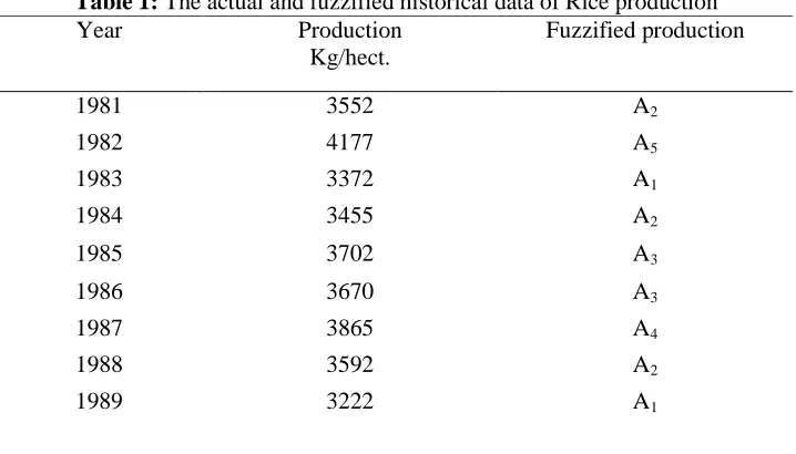
Step 4. The historical time series data are fuzzified and are placed in table 1.
Table 1: The actual and fuzzified historical data of Rice production
Year Production
Kg/hect.
Fuzzified production
1981 3552 A2
1982 4177 A5
1983 3372 A1
1984 3455 A2
1985 3702 A3
1986 3670 A3
1987 3865 A4
1988 3592 A2
Abhishekh and Sanjay Kumar
152
1990 3750 A3
1991 3851 A4
1992 3231 A1
1993 4170 A5
1994 4554 A7
1995 3872 A4
1996 4439 A7
1997 4266 A6
1998 3219 A1
1999 4305 A6
2000 3928 A4
2001 3978 A4
2002 3870 A4
2003 3727 A3
With these fuzzified productions, the fuzzy logical relations of various orders ( order 3, order 4, order 5 and so on) are constructed .
Table 2: Fourth order fuzzy logical relationships for the rice production are obtained as
Time Series
153
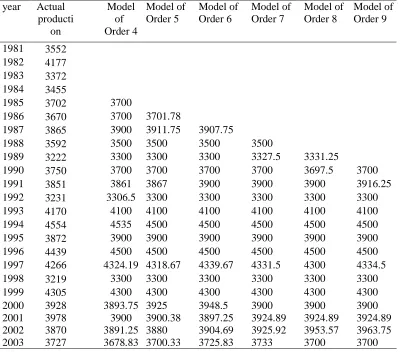
Step 5. The forecasted values have been obtained by using the algorithms in section 3. The forecasted production of Rice obtained by these methods is placed in the Table 3.
Table 3: Actual rice production vs forecasted outputs by proposed high–order models
year Actual producti
on
Model of Order 4
Model of Order 5
Model of Order 6
Model of Order 7
Model of Order 8
Model of Order 9
1981 3552
1982 4177
1983 3372
1984 3455
1985 3702 3700
1986 3670 3700 3701.78
1987 3865 3900 3911.75 3907.75
1988 3592 3500 3500 3500 3500
1989 3222 3300 3300 3300 3327.5 3331.25
1990 3750 3700 3700 3700 3700 3697.5 3700
1991 3851 3861 3867 3900 3900 3900 3916.25
1992 3231 3306.5 3300 3300 3300 3300 3300
1993 4170 4100 4100 4100 4100 4100 4100
1994 4554 4535 4500 4500 4500 4500 4500
1995 3872 3900 3900 3900 3900 3900 3900
1996 4439 4500 4500 4500 4500 4500 4500
1997 4266 4324.19 4318.67 4339.67 4331.5 4300 4334.5
1998 3219 3300 3300 3300 3300 3300 3300
1999 4305 4300 4300 4300 4300 4300 4300
2000 3928 3893.75 3925 3948.5 3900 3900 3900
2001 3978 3900 3900.38 3897.25 3924.89 3924.89 3924.89
2002 3870 3891.25 3880 3904.69 3925.92 3953.57 3963.75
2003 3727 3678.83 3700.33 3725.83 3733 3700 3700
The suitability of the proposed model in forecasting the rice production has been studied on the basis of mean square error (MSE) and average error of the forecast. The MSE is defined as
Mean Square Error =
n
value forecasted value
actual
n
i
i i
∑
=
− 1
2
) (
Abhishekh and Sanjay Kumar
154
Table 4: Mean square error and average error of rice production forecast of proposed models
Order of forecast
order 4 Order 5 Order 6 Order 7 Order 8 Order 9
Average Error
1.2396
16 1.265129 1.389997 1.46002 1.434785 1.397004
MSE 2881.2 2988.2 3442.2 3701.3 3548.9 3445.8
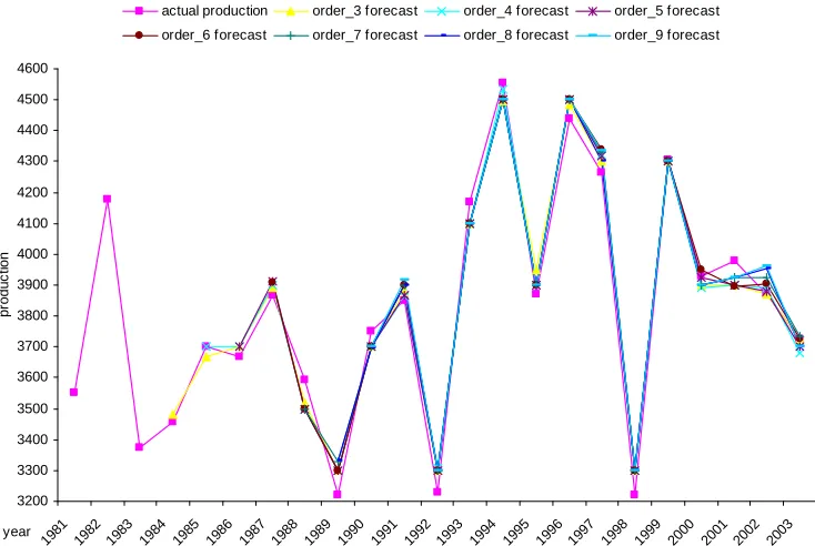
Further, the trends in forecast of the proposed model of these high-orders can examined with more clarity by the figure given below. One of the interesting features in the forecasting of rice production by the proposed high-order model can be visualized that the accuracy in forecasted values is of varying degree.
Figure 1: Actual rice production vs forecasted rice production by higher order model of proposed method.
5. Conclusions
The developed method is a computational method for various high-order forecasting based on the fuzzy time series and provides better results than the existing methods. The study reveals some interesting features of the high-order fuzzy time series forecasting that their suitability varies according to the fuzziness in the time series data. Forecasted values for some years in various high order models are invariant and may be considered a suitable forecast for the respective years. Thus an efficient and accurate forecasting also needs the computation of forecasting by various high orders, the proposed method being
Actual rice production vs f orecasted production by proposed high order models
3200 3300 3400 3500 3600 3700 3800 3900 4000 4100 4200 4300 4400 4500 4600
1981 1982 1983 1984 1985 1986 1987 1988 1989 1990 1991 1992 1993 1994 1995 1996 1997 1998 1999 2000 2001 2002 2003
year
p
ro
d
u
c
tio
n
Time Series
155
a computational method can be easily employed to get the forecasting of various high-orders more efficiently. Further, the implementation of fuzzy time series in crop production forecast is to support the development of decision support system in Agricultural production system, one of the real life problems falling in the category having uncertainty in known and unknown parameters. This study may be useful in the tactical and forecasting applications in agricultural decision support systems.
Acknowledgement
Author is highly thankful to The General Manager, Farms, Govind Ballabh Pant University of Agriculture and Technology, Pantnagar-263145, Udham Singh Nagar, (Uttarakhand), INDIA for providing the valuable time series data of crop (rice) production.
We also grateful to the reviewers for their constructive comments.
REFERENCES
1. C.H.Cheng, Fuzzy time series based on adaptive expectation model for TAIEX forecasting, Expert Systems with Applications, 34 (2008) 1126-1132.
2. S.M.Chen, Forecasting enrollments based on fuzzy time series. Fuzzy Sets and Systems, 81(1996) 311-319.
3. S.M.Chen, Forecasting enrollments based on high-order fuzzy time series, Cybernetics and systems: An International Journal, 33 (2002) 1-16.
4. S.M.Chen and J.R.Hwang, Temperature prediction using fuzzy time series, IEEE Transactions on Systems, man, and Cybernetics-Part B: Cybernetics 30 (2000) 263- 275.
5. S.M.Chen and C.C.Hsu, A new method to forecast enrollments using fuzzy time series, International Journal of Appl. Sciences and Engg., 2 (2004) 234-244.
6. C.H.Cheng, J.R.Chang and C.A.Yeh, Entropy- based and Trapezoid fuzzification-based fuzzy time series approaches for forecasting IT project cost, Technological Forecasting and Social Change, 73 (2006) 524-542.
7. S.H.Cheng, S.M.Chen and W.S. Jian, Fuzzy time series forecasting based on fuzzy logical relations and similarity measures, Information Sciences, 327 (2016) 272-287. 8. S.S.Gangwar and S.Kumar, Partition based computational method for high order
fuzzy time series forecasting, Expert Systems with Applications, 39 (2012) 12158-12164.
9. K.Huarng, Heuristic models of fuzzy time series for forecasting, Fuzzy Sets and Systems, 123 (2001) 369-386.
10. K.Huarng and T.H.K.Yu, Ratio-based lengths of intervals to improve fuzzy time series forecasting, IEEE Trans on SMC –Part B: Cybernetics 36 (2006) 328-340. 11. J.R.Hwang, S.M.Chen and C.H.Lee, Handling forecasting problems using fuzzy
time series, Fuzzy Sets and Systems, 100 (1998) 217-228.
12. Z.Ismail and R Efendi, Enrollment forecasting based on modified weight fuzzy time series, Journal of Artificial Intelligence, 4(1) (2011) 110-118.
Abhishekh and Sanjay Kumar
156
14. I.Kim and S.R. Lee, A fuzzy time series prediction method based on consecutive values, IEEE International Fuzzy Systems Conference, August 22-25, Seol Korea, Proceedings II : (1999) 703-707.
15. H.S.Lee and M.T.Chou, Fuzzy forecasting based on fuzzy time series, International Journal of Computer Mathematics, 81(2004) 781-789.
16. L.W.Lee, L.H.Wang and S.M. Chen, Handling forecasting problems based on two-factor high-order fuzzy time series, IEEE Transactions on Fuzzy Systems, 14(3) (2006) 468-477.
17. M.H.Lee, R.Efendi and Z.Ismail, Modified weighted for enrollment forecasting based on fuzzy time series, MATEMATIKA, 25(1) (2009) 67-78.
18. S.T.Li and Y.P.Chen, Natural partitioning-based forecasting model for fuzzy time series, FUZZ-IEEE -2004 Hungry, IEEE (2004) 1355-1359.
19. C.M.Own and P.T.Yu, Forecasting fuzzy time series on a heuristic high-order model, Cybernetics and Systems:An International Journal, 36 (2005) 705-717.
20. W.Qiu, X.Liu and H.Li, A generalized method for forecasting based on fuzzy time series, Expert Systems with Applications, 38 (2011) 10446-10453.
21. P.Singh and B.Borah, An efficient time series forecasting model based on fuzzy time series, Engineering Applications of Artificial Intelligence, 26 (2013) 2443-2457. 22. S.R.Singh, A simple method of forecasting based on fuzzy time series, Applied
Mathematics and Computation,186 (2007) 330-339.
23. S.R.Singh, A robust method of forecasting based on fuzzy time series, Applied Mathematics and Computation , 188 (2007) 472-484.
24. S.R.Singh, A simple time variant method for fuzzy time series forecasting, Cybernetics and Systems:An International Journal, 38 (2007) 1-17.
25. Q.Song and B.S.Chissom, Fuzzy time series and its models, Fuzzy Sets and Systems, 54 (1993) 269-277.
26. Q.Song and B.S.Chissom, Forecasting enrollments with fuzzy time series–Part I, Fuzzy Sets and Systems, 54 (1993) 1-9.
27. Q.Song and B.S.Chissom, Forecasting enrollments with fuzzy time series–Part II, Fuzzy Sets and Systems, 64 (1994) 1-8.
28. J.Sullivan and W.H.Woodall, A comparison of fuzzy forecasting and Markov modeling, Fuzzy Sets and Systems, 64 (1994) 279- 293.
29. C.C.Tsai and S.J.Wu, A study for second-order modeling of fuzzy time series, IEEE International Fuzzy Systems Conference Proceedings Aug 22-25,1999 Seoul, Korea, IEEE:II (1999) 719-725.
30. C.C.Tsai and S.J.Wu, Forecasting local region data with fuzzy time series, ISIE 2001,Pusan, KOREA, Proceedings, IEEE (2001) 122-133.
31. C.C.Tsai, S.J.Wu and W.H.Ting, On the effect of membership function in a high-order fuzzy time series, IEEE International Fuzzy Systems Conference Proceeding, IEEE (2002) 437-442.
32. R.C.Tsaur, J.C.O.Yang and H.F.Wang, Fuzzy relation analysis in fuzzy time series model , Computer and Mathematics with Applications, 49(2005) 539-548.
33. V.R.Uslu, E.Bas, U.Yolcu and E.Egrioglu, A fuzzy time series approach based on weights determined by the number of recurrences of fuzzy relations, Swarm and Evolutionary Computation, 15 (2014) 19-26.
Time Series
157
series forecasting, IEEE Transactions on System, Man, and Cybernetics-Part B; Cybernetics, 40(6) (2010) 1531-1542.
35. S.Xihao and L.Yimin, Averaged–based fuzzy time series models for forecasting Shanghai compound index, World Journal of Modelling and Simulation, 4(2) (2008) 104-111.
36. H.K.Yu, A refined fuzzy time series model for forecasting, PHYSICA A, 346 (2005) 657-681.
37. H.K.Yu, Weighted fuzzy time series model for TAIEX forecasting, PHYSICA A, 349 (2005) 609-624.
38. L.A.Zadeh, Fuzzy Set, Information and Control, 8 (1965) 338-353.