Consumption using Gaussian Processes
Milindanath Samarasinghe and Waseem Al-Hawani
Supervisor Ole-Christoffer Granmo
This Master’s Thesis is carried out as a part of the education at the University of Agder and is therefore approved as a part of this education. However, this does not imply that the
University answers for the methods that are used or the conclusions that are drawn.
University of Agder, 2012 Faculty of Engineering and Science
Forecasting of electricity consumption is considered as one of the most significant aspect of effective management of power systems. On a long term basis, it allows decision makers of a power supplying company to decide when to build new power plants, transmission and distri-bution networks. On a short term basis, it can be used to allocate resources in a power grid to supply the demand continuously.
Forecasting is basically divided into three categories : short-term,medium-term, and long-term. Short-term refers to an hour to a week forecast, while medium-term refers to a week to a year, and predictions that run more than a year refers to long-term.
In this thesis, we forecast electricity consumption on a short-term basis for a particular region in Norway using a relatively novel approach: Gaussian process. We design the best feature vector suitable for forecasting electricity consumption using various factors such as
previous consumptions, temperature, days of the week and hour of the day. Moreover, feature space is scaled and reduced using reduction and normalization methods, and different target variables are analysed to obtain better accuracy.
Furthermore, GP is compared with two traditional forecasting techniques : Multiple Back-Propagation Neural Networks (MBPNN), and Multiple Linear Regression (MLR). Finally we show that GP is as better as MBPNN and far better than MLR using empirical results.
This thesis is submitted in partial fulfilment of the degree of Master of Science in Information and Communication Technology (ICT) at University of Agder, Grimstad, Norway. The thesis was carried out under the supervision of professor Ole-Christoffer Granmo. We are delighted to take the opportunity to thank all the people who have made valuable support in completing this work.
Professor Ole-Christoffer Granmo was the strong guiding force in our work, who led us in the correct path towards achieving our final goal. His knowledge and experience in the field and the willingness to share his insights with us in this research was remarkable. Therefore we are grateful to him for all that support. We should also thankful to Eidsiva Energy for providing the dataset that was the basic foundation of our thesis. Our acknowledgement also goes to Noel Lopes for providing his research paper for the neural network testing. Finally, we would like to pay our gratitude to our fellow students who helped us in numerous ways to make this thesis a success.
Grimstad, May 2012
Milindanath Samarasinghe Waseem Al-Hawani
Contents iii
List of Figures vi
List of Tables ix
1 Introduction 1
1.1 Background and Motivation . . . 1
1.2 Thesis Definition . . . 4 1.3 Research Questions . . . 4 1.4 Research Approach . . . 5 1.5 Contributions . . . 6 1.6 Target Audience . . . 6 1.7 Thesis Outline . . . 6
2 Electricity Consumption and Forecasting 8 2.1 Electricity Supplying Process . . . 8
2.2 Electricity Consumption . . . 9
2.3 Electricity Consumption Forecasting . . . 10
3 Gaussian Process and Regression 12 3.1 Random Variables . . . 12
3.1.1 Cumulative Distribution Function . . . 12
3.1.2 Probability Density Function . . . 13
3.2 Gaussian Probability Distribution . . . 14
3.3 Gaussian Process . . . 14
3.3.1 Mean Function . . . 15
3.3.2 Covariance Function . . . 15
3.4 Regression Analysis . . . 16
3.5 Gaussian Process Regression . . . 17
3.5.1 Selection of Hyperparameters . . . 21
4 Traditional Approaches of Electricity Consumption Forecasting 22 4.1 Artificial Neural Networks . . . 22
4.1.1 Introduction to ANN . . . 22
4.1.2 Back-Propagation Neural Networks . . . 23
4.1.3 Multiple Back-Propagation . . . 28
4.2 Linear Regression . . . 29
4.2.1 Statistical Significance . . . 29
4.2.2 Linear Regression . . . 30
4.2.3 Multiple Linear Regression . . . 34
5 Short-term Forecasting of Electricity Consumption using GP 36 5.1 Cyclic Patterns of Consumption . . . 36
5.1.1 Hourly Consumption on Annual Basis . . . 36
5.1.2 Hourly Consumption on Seasonal Basis . . . 38
5.1.3 Hourly Consumption on Weekly Basis . . . 38
5.2 Feature Vector Design . . . 44
5.3 Target Variable Analysis . . . 45
5.4 Feature Space Reduction and Normalization . . . 46
5.5 Kernel Function . . . 47
6 Experiments and Results 49 6.1 Gaussian Process . . . 49
6.1.1 Dynamic Training Dataset - Original Data . . . 50
6.1.2 Dynamic Training Dataset - Kernel Reduced Data . . . 52
6.1.3 Dynamic Training Dataset - Normalized Data . . . 54
6.1.4 Fixed Training Dataset - Original Data . . . 56
6.1.5 Fixed Training Dataset - Kernel Reduced Data . . . 57
6.1.6 Fixed Training Dataset - Normalized Data . . . 57
6.1.7 Next 24 Hours Prediction . . . 58
6.2 Traditional Approaches . . . 60
6.2.1 MBPNN - Original Data . . . 60
6.2.2 MBPNN - Normalized Data . . . 61
6.2.3 Multiple Linear Regression . . . 61
7 Discussion and Summary of Results 71 7.1 Cyclic Patterns . . . 71
7.2 Dynamic Training Dataset . . . 72
7.3 Fixed Training Dataset . . . 74
7.3.1 Next 24 Hours Prediction . . . 78
7.4 Comparison between GP and Traditional Approaches . . . 78
8 Conclusion and Further Work 81 8.1 Conclusion . . . 81
8.2 Further Work . . . 82
Glossary and Abbreviation 88
A Screen-shots of MBP Software 90
1.1 Earth at night. [Source : NASA]. . . 1
1.2 Electricity consumption by user group in Norway, 1990-2007 [1]. . . 2
2.1 A typical power system with generation, transmission and distribution phases. [Source: http://science.howstuffworks.com/environmental/energy/power.htm]. . . 9
2.2 Electricity consumption for 2008, 2009 and 2010. The vertical dashed lines sep-arate the three years consecutively, and the x axis shows the cumulative hours starting from January 1st 2008. . . 10
3.1 Illustration of Cumulative Distribution Function. . . 13
3.2 Gaussian Probability Distribution. . . 14
3.3 A set of sample training data points with one test data point whose target value is unknown. . . 17
3.4 A set of sample training data points with the predicted target value of the test data point. . . 20
4.1 A typical neuron in a biological nervous system. . . 23
4.2 A typical feed-forward network used for back-propagation . . . 24
4.3 The logistic function which is one type of sigmoid functions. . . 25
4.4 A BPNN with weights and bias values. Neurons are represented by circles and bias by triangles. . . 26
4.5 A Multiple feed-forward network. Hidden and output neurons are represented by circles, input neurons by squares, and bias by triangles [2]. . . 29
4.6 Scatter plot of the sample dataset. . . 30
4.7 Fitted line for the sample dataset. . . 32
4.8 The normal P-P plot of regression, which is used for residual analysis. . . 33
4.9 Graph of standardized predicted value versus standardized residual value, which is used for residual analysis. . . 33
5.1 Time horizon hierarchy. . . 37
5.2 Mean hourly electricity consumption in 2008, 2009 and 2010. . . 37
5.3 Mean hourly electricity consumption for different seasons in 2008. . . 39
5.4 Mean hourly electricity consumption for different seasons in 2009. . . 39
5.6 Mean hourly electricity consumption on Mondays in year (a) 2008 (b) 2009 and (c) 2010. . . 40 5.7 Mean hourly electricity consumption on Tuesdays in year (a) 2008 (b) 2009 and
(c) 2010. . . 41 5.8 Mean hourly electricity consumption on Fridays in year (a) 2008 (b) 2009 and
(c) 2010. . . 42 5.9 Mean hourly electricity consumption on Saturdays in the year (a) 2008 (b) 2009
and (c) 2010. . . 43 5.10 Mean hourly electricity consumption on Sundays in year (a) 2008 (b) 2009 and
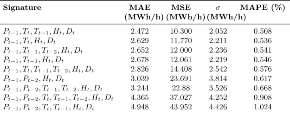
(c) 2010. . . 44 6.1 Actual and predicted electricity consumptions of the combinationPt−1TtTt−1HtDt
for the original data set with δPt as the target variable. . . 51
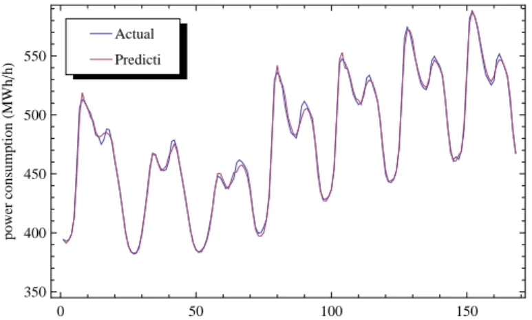
6.2 Actual and predicted electricity consumptions of the combinationPt−1TtTt−1Tt−2HtDt
for the original data set with Pt as the target variable. . . 52
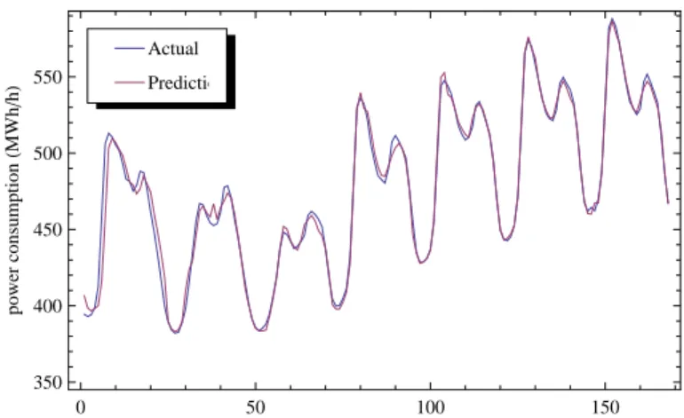
6.3 Actual and predicted electricity consumptions of the combinationPt−1TtTt−1HtDt
for the kernel reduced data set with δPt as the target variable. . . 53
6.4 Actual and predicted electricity consumptions of the combination Pt−1HtDt for
the kernel reduced data set with Pt as the target variable. . . 54
6.5 Actual and predicted electricity consumptions of the combinationPt−1TtTt−1HtDt
for the normalized data set withδPtas the target variable. . . 55
6.6 Actual and predicted electricity consumptions of the combinationPt−1Pt−2TtTt−1Tt−2HtDt
for the normalized data set withPtas the target variable. . . 56
6.7 The (a) MAE and (b) MAPE curves for the next 24 hours predictions for the best
combinations in the four seasons. Pt−1TtTt−1Tt−2HtDtfor winter,Pt−1Pt−2TtTt−1Tt−2HtDt
for spring, Pt−1Pt−2TtTt−1HtDtfor summer and Pt−1Pt−2TtTt−1HtDt for autumn. 60
7.1 Execution time for each best prediction in the six categories. . . 72 7.2 Usage of the variables Pt−2, Tt, Tt−1 and Tt−2 for the best results with an MAE
less than 3.0. . . 73 7.3 Usage of the variablesPt−2, Tt, Tt−1 and Tt−2 in the top 10 predictions of winter
season. . . 74 7.4 Usage of the variables Pt−2, Tt, Tt−1 andTt−2 in the top 10 predictions of spring
season. . . 75 7.5 Usage of the variablesPt−2, Tt, Tt−1 andTt−2in the top 10 predictions of summer
season. . . 76 7.6 Usage of the variablesPt−2, Tt, Tt−1andTt−2 in the top 10 predictions of autumn
season. . . 77 7.7 Usage of variables Pt−2Tt, Tt−1 and Tt−2 in top 10 predictions for all the seasons. 77
7.8 The (a) MAE and (b) MAPE curves for the next 24 hours predictions for the best combinations in the four seasons. Pt−1, Tt, Tt−1, Tt−2, Ht, Dt for winter, Pt−1, Pt−2, Tt, Tt−1, Tt−2, Ht, Dt for spring, Pt−1, Pt−2, Tt, Tt−1, Ht, Dt for
A.1 The main screen of defining the neural network to be tested . . . 90 A.2 Output of the training dataset . . . 91 B.1 The mean hourly electricity consumption on Wednesdays in year (a) 2008 (b)
2009 and (c) 2010 . . . 92 B.2 The mean hourly electricity consumption on Thursdays in year (a) 2008 (b) 2009
3.1 Sample dataset for regression. . . 17
4.1 Variables table. . . 31
4.2 Model summary table. . . 31
4.3 ANOVA table. . . 31
4.4 Coefficients table. . . 32
4.5 Correlation for multiple variables. . . 34
4.6 Coefficients for multiple variables. . . 34
5.1 Seasons and their durations. . . 38
5.2 Variables considered in the feature vector and their notations. . . 45
5.3 Differences of mean power consumption (MWh/h) between successive hours of the 3 years . . . 46
5.4 Range of values of different predictor variables in 2008. . . 47
6.1 Fixed training and test datasets. . . 50
6.2 Results for the prediction of power difference for original dataset. . . 50
6.3 Results for the prediction of power consumption for original dataset. . . 51
6.4 Results for the prediction of power difference for kernel reduced dataset. . . 52
6.5 Results for the prediction of power consumption for kernel reduced dataset. . . . 53
6.6 Results for the prediction of power difference for normalized dataset. . . 54
6.7 Results for the prediction of power consumption for normalized dataset. . . 55
6.8 Results for the prediction of power difference for original dataset on seasonal basis. 57 6.9 Results for the prediction of power difference for kernel reduced dataset on sea-sonal basis. . . 57
6.10 Results for the prediction of power difference for normalized dataset on seasonal basis. . . 58
6.11 Results for the prediction of power difference for next 24 hours in winter. . . 58
6.12 Results for the prediction of power difference for next 24 hours in spring. . . 59
6.13 Results for the prediction of power difference for next 24 hours in summer. . . . 59
6.14 Results for the prediction of power difference for next 24 hours in autumn. . . 59
6.15 Results for the prediction of power difference in MBPNN with 10 hidden layer neurons and 10000 epochs. . . 61
6.16 Results for the prediction of power difference in MBPNN with 10 hidden neurons
and 10000 epochs. . . 61
6.17 Coefficients table for winter. . . 62
6.18 ANOVA table for winter. . . 62
6.19 Model summary table for winter. . . 63
6.20 Results for the prediction of power consumption for winter using MLR. . . 63
6.21 Coefficients table for spring. . . 64
6.22 ANOVA table for spring. . . 65
6.23 Model summary table for spring. . . 65
6.24 Results for the prediction of power consumption for spring using MLR. . . 66
6.25 Coefficients table for summer. . . 66
6.26 ANOVA table for summer. . . 67
6.27 Model summary table for summer. . . 67
6.28 Results for the prediction of power consumption in summer using MLR. . . 68
6.29 Coefficients table for summer. . . 68
6.30 ANOVA table for autumn. . . 69
6.31 Model summary table for autumn . . . 69
6.32 Results for the prediction of power consumption in autumn using MLR. . . 70
7.1 Best forecasting results of the six categories for the dynamic dataset. . . 72
7.2 Top 10 forecasting results for dynamic dataset. . . 73
7.3 Top 10 forecasting results for winter. . . 74
7.4 Top 10 forecasting results for spring. . . 75
7.5 Top 10 forecasting results for summer. . . 76
7.6 Top 10 forecasting results for autumn. . . 76
7.7 Comparison of the forecasting results for winter. . . 79
7.8 Comparison of the forecasting results for spring. . . 79
7.9 Comparison of the forecasting results for summer. . . 79
7.10 Comparison of the forecasting results for autumn. . . 80
8.1 Best feature vectors. . . 82
8.2 Effect of previous consumption differences in the feature vector of the original dataset. . . 82
Introduction
In this chapter we direct the reader to the basic introduction of the thesis. In section 1.1, we outline the basic background and motivation of the thesis. We define the thesis definition in section 1.2 and present the basic research questions need to be solved in section 1.3. The remaining three sections: section 1.5, 1.6 and 1.7 detail the contributions supplemented to the research community; the target audience of the thesis; and the outline of the thesis respectively.
1.1
Background and Motivation
Electricity has become a basic need for the mankind today. It is used to carry out a range of day to day work, such as operating domestic and industrial equipments, lighting, heating, air-conditioning, cooking, washing and many other tasks. We can visualize this fact of how it
Figure 1.2: Electricity consumption by user group in Norway, 1990-2007 [1].
has become a basic need for mankind, by just looking at the earth at night in Figure 1.1, which illustrates the electricity required to light the earth at night.
This is true for the Norwegian community also, as we can see from Figure 1.2, which illus-trates the electricity consumption among different user groups in Norway from 1990 to 2007. The figure indicates an increase in consumption for many user groups over the years. Therefore it is clear that electricity has become an important commodity for the people.
Forecasting of electricity consumption is necessary to manage the power system effectively and thereby fulfil this increasing demand. On a long-term basis, power companies would require the power consumption forecast in the next 10 or 20 years to plan their future activities prop-erly, such as building adequate power plants and improve their transmission and distribution networks to meet the necessary demand. On a short-term basis, forecasting is required to per-form daily operations such as unit commitment, energy transfer scheduling and load dispatch of a utility company [3]. Therefore, accurate prediction of electricity consumption is crucial for both, performing daily operations and making future power plans for a power supplying company.
Electricity forecasting can be done mainly in three ways, as short-term, medium-term and
long-term. Short-term forecasting refers to an hour to a week prediction, while medium-term considers the range between a week and a year, and predictions that run more than a year are considered as long-term forecasts [4].
In the literature, we can observe various independent variables (predictors), that influence the consumption, have been used for forecasting under these three schemes, especially for short-term and long-short-term. In long-short-term forecasting, the most frequently used predictors are the
Gross Domestic Product (GDP) [5–8] and the population [5, 6, 8]. In addition, factors such as
capital [5],per capita consumption [6],number of consumers [6],peak electricity demand [6] and
temperature[9–11] andhumidity[9,11] have been widely used andwind-force[10],dampness[10],
chilled water consumption [9] andgas fuel consumption [9] have also been used for forecasting. The most common approaches of electricity consumption forecasting includes, statistical techniques (multiple linear regression), artificial neural networks (ANN) , Genetic algorithms (GA) , grey methods (GM) and time series analysis. Here, we briefly outline some of those selected attempts as follows. A statistical technique - multiple regression analysis using least squares method has been used by Imitiaz et al. [6] to forecast annual electricity consumption for Malaysia. Fung and Tummala [8] have used ANN models to forecast annual consumption and compared the results with multiple linear regression models. Dedy et al [9] have also used ANN to forecast daily electricity consumption by optimizing its model using Taguchi [12] method. RBF neural networks combined with Genetic algorithms have been used by Zeng et al. [10] for short-term forecasting. Grey methods [13] have been applied to forecast electricity consumption in [5]. A time series analysis based on auto regressive model done by Wang Baosen et al. [7] has been carried out for long-term electricity consumption forecasting.
In this thesis our approach is to forecast short term electricity consumption on an hourly basis which extends up to predicting the behaviour of the next 24 hours, using a relatively novel approach : Gaussian Process (GP) .
GP possess several attributes that make it a potential model to solve supervised learning problems which emerged over the last decade. The main reason for this is its non-parametric, kernel based nature, which provides more flexibility in solving inferring problems. GP is more a data-oriented approach which is capable of learning functions from the data itself. Moreover, it can be used for non-linear regression problems which makes it more suitable for forecasting electricity which is non linear in nature.
Gaussian process has been used before in a range of fields especially for estimating purposes. Here we concentrate on several of these researches. Gaussian processes has been used by Luo and Qian [14] to estimate the colour values in Poly Ethylene Terephthalate (PET) . Vathsangam et al. [15] have used GPs to estimate walking speed of a human using on-body accelerometers and gyroscopes. As Pasolli et al. propose in [16], it has been also used for estimating chlorophyll concentration in subsurface waters by sensing data remotely. According to Bazi and Melgani [17], semi-supervised GPs has been used for the estimation of biophysical parameters from remote sensing data. Zhang and Yeung [18] have suggested, Multi-Task Warped Gaussian Process (MTWGP) , which is a variant of GP, for personalized age estimation of people.
GP has been used for short-term electricity forecasting on two occasions in the literature. Firstly, by Mori and Ohmi [11], and secondly by Alamaniotis et al. [4]. In the first, GP has been used to forecast daily consumption and hierarchical Bayesian model has been used to evaluate the hyperparameters of the covariance function. Moreover, they have compared GP with conventional methods such as MLP , RBFN and SVR . In the second, several kernel functions have been built and the predictors have been evaluated using Genetic algorithm.
In our approach, we use GP on its original context but more focusing on the data itself by modifying both feature vector and target variable. We use techniques such as reduction and
normalization to modify the feature vector and test for different target variables that gives better results. Moreover, we compare GP with two traditional techniques: multiple linear regression
(MLR) and multiple back-propagation neural networks (MBPNN) , which have not been used in [11]. More focus will be given to seasonal changes in consumption, as there is a tie between weather and consumption in a country like Norway. Therefore, it is interesting to see how GP cope with these variations as it has been found in [19] that, traditional techniques such as linear regression and NN are not much sensitive to variations in the local structure of the input space and hence we can examine the ability of GP in estimating varying electricity consumption. However as stated clearly by Imitiaz et.al [6], forecasts are never going to be perfect and the validity of the general rule ’The forecast is always wrong’ has to be assumed.
1.2
Thesis Definition
The thesis definition can be formulated as follows:
This thesis proposes Gaussian Processes (GP) as a novel approach for short term forecasting of electricity consumption. It includes designing the optimum feature vector by concerning various factors affecting the electricity consumption. This should consist of a data filtering strategy and data scaling technique. In addition, it is required to use a corresponding kernel function for achieving best predictions. The core of the thesis is the design of a technique for exploring trends of electricity consumption through cyclic patterns and hence normalize the data in such a way that accurate predictions could be obtained. Moreover, it is expected to compare the forecast results of GP with the traditional forecasting techniques.
1.3
Research Questions
Throughout this thesis, we will answer to the research questions outlined below.
What are the cyclic patterns that we can observe in electricity consumption and what are the influential factors causing these cycles?
Electricity consumption will be different from hour to hour, day to day, month to month, season to season and year to year. But they can have repeating cyclic patterns. For this purpose, we consider a dataset, provided by Eidsiva Energy1 which contains electricity consumption data for 3 years. Using this dataset, we have to find out the patterns of electricity consumption and the factors that influence these patterns.
1
What is the best feature vector possible for forecasting electricity consumption under GPs?
As we know, electricity consumption may depend on many factors as mentioned in section 1.1. In our approach we focus mainly on the weather factors(temperature, wind, cloud cover), season of the year (summer, autumn, spring, winter), days of the week, hours of the day and previous electricity consumption values. The most influencing factors could be identified once we answer the first research question about cyclic patterns, and studying more about the dataset. Hence we could identify a feature vector(s) that is more suitable to obtain better prediction results.
What type of target variables we can use for better prediction accuracy?
It is obvious that the electricity consumption is the default target variable. However, we need to explore another target variable(s) which is(are) capable of providing better results. This would require a thorough emphasis on the dataset.
What are the strategies used to improve the predictions?
We need to test different techniques, and features to find out the best possible combinations of the input feature space that produce the accurate results. This might include scaling, normal-izing and reducing methods.
How good the predictions of GP compared with the traditional techniques?
It is necessary to compare the results of GP with the traditional techniques used to forecast electricity consumption. Here, we propose two traditional techniques : multiple linear regression
and multiple back-propagation neural networks.
1.4
Research Approach
The main starting point for this thesis is the dataset obtained from Eidsiva Energy as mentioned above. This dataset consists hourly electricity consumption measured in three successive years 2008, 2009 and 2010. In addition to the electricity consumption, temperature, cloud cover, wind speed are also stated in this dataset.
Through extensive studies on the dataset, we answer the research questions outlined above one by one using GP. Dataset will be utilized under different categories based on their attributes and features.
GP testing is done using the pyXGPR [35] python code library developed by Marion Neu-mann et al. This tool is based on the GP theories explained by Rasmussen and Williams [26].
1.5
Contributions
In this thesis, we introduce Gaussian process as a novel approach for short-term electricity forecasting on a seasonal basis, for a region where electricity consumption is related with the weather condition. The best feature vectors for forecasting electricity consumption on seasonal basis are found using the weather factors, previous electricity consumptions, days of the week, and hour of the day.
In addition to the input feature space, this thesis tests for different target variable analysis, to obtain better results.
Moreover, we evaluate the results of GP when reduction and normalization methods are applied to the feature space, in terms of electricity forecasting.
Finally, GP is compared with two traditional techniques : multiple linear regression and multiple back-propagation neural networks, which have not been compared in [11]. This will allow us to examine how good GP process compared with the other techniques.
1.6
Target Audience
This thesis can be referred by anyone who is interested in the machine learning field. Specially for those who have interest in the emerging technique of Gaussian processes.
Those who are in electric utility companies might be very much interested in forecasting electricity consumption. Therefore, this thesis work will be beneficial for them who are seeking improvements in their electricity supplying process.
In general, anyone who is working with the computer science, electrical engineering and statistics can use this thesis as a reference. However the readers are assumed to have the background knowledge on statistics theory and machine learning.
1.7
Thesis Outline
Mainly, the thesis is organized into eight chapters as follows. Chapter 1 covers the basic in-troductory part of the thesis, the background and motivation ,the research questions that we should solve, the thesis definition, contributions to the knowledge and the target audience.
Chapter 2 illustrates how the electricity generation, transmission and distribution process works, the consumption patterns of the consumers and the previous approaches of forecasting. Chapter 3 covers the basic theoretical background of GP and GP regression, with a short introduction to the random variable theories.
electricity forecasting: linear regression and artificial neural networks.
Chapter 5 is concerned with the proposed solution on how to forecast electricity consumption using Gaussian processes. Chapter 6 outlines the empirical results obtained from different tests including GP and traditional methods. Chapter 7 analyses the results obtained and compare GP with the traditional techniques. Finally, Chapter 8 concludes the findings by exploring the whole thesis work.
Electricity Consumption and
Forecasting
In chapter 1, we gave a brief introduction about the background of electricity consumption forecasting, with the traditional forecasting techniques and the need of Gaussian process. How-ever, first we should understand the basics of an actual power system and how it processes in the practical situation and how forecasting is going to do any good for the improvement of the system. In section 2.1, we discuss some of the theoretical features of a typical power system and how it fits with our case. Then we move on to the consumption of electricity, produced by the system based on our dataset and the different features of consumption in section 2.2. In the last section we discuss the importance of forecasting and give some details about the previous approaches in forecasting.
2.1
Electricity Supplying Process
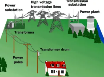
There is a complex process associated in delivering electricity safely and reliably to house-holds and industries. This process involves three basic stages : generation, transmission and distribution. Figure 2.1 illustrates these three stages in a typical electric power system.
The root of power generation is the power plant, which includes turbines and generators. There are different types of power plants based on the source of energy, such as hydro power, thermal, wind, solar and so on. The main source of electricity in Norway is the hydro-power and it constitutes 99 % of the overall production [20].
Figure 2.1: A typical power system with generation, transmission and distribution phases. [Source: http://science.howstuffworks.com/environmental/energy/power.htm].
In the next stage, three-phase power generated by this power plant is transmitted to a long distance through high voltage transmission lines as shown in the figure. Before transmitting, the voltage of the generated power, is increased (step-up) by the transformers in the transmission substation.
These transmission lines are then connected to power substations where the high voltage power is stepped down to a level that can be distributed across a certain region. This step is the last stage of the power system which is also known as the distribution stage. From the distribution transformer, the distribution bus lines carries electricity to the households and industries.
In short-term electricity forecasting, the main focus goes to the distribution stage. This is because, the controlling process could be only carried out on this stage by allocating proper resources on a short-term basis.
2.2
Electricity Consumption
In Norway, the authorities who distribute electricity from the final stage of the process are keen to provide better and continuous supply to their consumers all the time. In this process, they have to control and monitor the distribution of electricity through their grids according to the demand from the consumers.
Eidsiva Energy records the power consumption in the region on an hourly basis. In addition to the power consumption, the forecast temperature, actual temperature, wind speed and cloud cover are also measured with the consumption. These measurements which we found in the dataset are the basis for the forecasting carried out in this thesis.
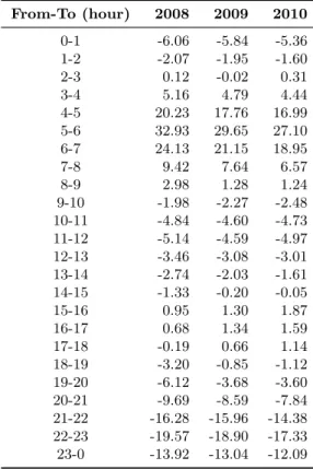
Figure 2.2 depicts the electricity consumption for the three years: 2008, 2009 and 2010 in the considered dataset.
0 5000 10 000 15 000 20 000 25 000 100 200 300 400 500 600 cumulative hours power consumption H MWh h L
Figure 2.2: Electricity consumption for 2008, 2009 and 2010. The vertical dashed lines separate the three years consecutively, and the x axis shows the cumulative hours starting from January 1st 2008.
According to the figure we can see that, there is a clear pattern in the consumption through-out a year. Winter (rare ends of each graph) and summer (middle section of each graph) seasons could be clearly visible in the figure with identical consumptions. The average power consump-tion in 2008 is 319.344 MWh/h and for 2009 it is 300.442 MWh/h and 304.407 MWh/h for 2010. Therefore it seems to be in the range of early 300. Moreover, we can see from figure that the power normally ranges from 100 to 600.
The weather factors seem to be playing a big role in these consumptions, due to the sea-sonal variations in the graph. Temperature is the most influential factor in terms of seasea-sonal changes. Therefore, we specially focus on theforecast temperature as it is the most influential environmental factor that affects the electricity consumption [21].
2.3
Electricity Consumption Forecasting
Forecasting of electricity consumption enables power utility companies to distribute electricity effectively. Electricity cannot be stored once it is generated. Therefore, it is very important to know how much electricity should be bought and distributed through the grid to the households and industries. Knowing the future consumption allows to manage this process in an effective way.
Therefore most power supplying companies and researchers have studied about different techniques to accurately forecast electricity consumption over the past few decades. Therefore we conclude this chapter by explaining how previous researches have been carried out regarding electricity consumption forecasting.
The research conducted by Imitiaz et al. [6] have used statistical analysis, which is basi-cally linear regression, to evaluate and forecast long term electricity consumption demand for Malaysia. They have used factors such aspopulation,per capita electricity consumption,number of consumers, peak electricity demand and GDP as the independent variables that affects the consumption. They have used training data of 10 years (from 1993-2003) to forecast for 7 years ahead (2004-2013).
As shown in [7], time series analysis based on autoregressive models has been used as another technique to predict power consumption. Time series analysis is a very popular technique for prediction. However it assumes that the past trends remain same for the future in estimating future values. The time series in this research has been based on the autoregressive model which express the value of a certain variable as a linear function of its previous values. They have used data from 1998 - 2005 as training, and 2006 - 2010 as test data. In our method also, we will adopt some of this technique in determining the feature vector as described in chapter 5.
From the range of methods used, grey methods [13] have also been a major consideration in terms of power prediction. Two models in grey methods: GM(1,1) and GM(0,N) have been used to forecast power consumption in a research done by Fang et.al [5].
In addition to these approaches, one of the most widely used techniques to predict power consumption is the neural networks as suggested in [8, 22, 23]. The research done by Fung and Tummala [8] compares the techniques, multiple linear regression and artificial neural network models, and concludes that ANN forecasts are at least as good as those generated by the multiple linear regression model. For ANN, they have used delta rule learning and error propagation methods to train the network. Different training and test datasets have been used in the span from 1970 - 1992.
Moreover, these two methods have also been used by Dhulst et al. [22] to predict the electric load consumed at a substation in Belgian electricity grid. In addition to that Quing et al. [23] suggests genetic algorithm and RBF neural network can be used to forecast power consumption, in which, GA optimizes the parameters of RBF neural network.
If we consider using of Gaussian processes in electricity consumption forecasting, we can find mainly two researches. The first one done by Alamaniotis and Ikonomopoulos [4], in which they apply genetic algorithm to determine the contribution from each independent predictor variable in order to compute a Pareto optimal solution. In this, they have used a set of kernels(will be defined in the next chapter) in the model. The kernel used in this technique are Neural Net,
Mat´ern, andRational Quadratic. The second, conducted by Mori and Ohmi [11] used Gaussian processes for daily power forecasting and a comparison has been done with MLP, RBFN and SVR.
Gaussian Process and Regression
In this chapter we move on to the theoretical aspects of the main research area in this thesis -Gaussian Processes. Before explaining that, we point to give a basic understanding about the basics of random variables and Gaussian probability distribution. In section 3.3, we explain about GP and in the following sections detail how the regression process is done using GP.
3.1
Random Variables
The concept of random variable can be explained by means of an experiment specified by the space S. A random variable (RV) is a number X(s) assigned to every outcome sS of that particular experiment [24]. In fact, the random variable X is a function whose domain issand the range is the real numbersR. It could be mathematically expressed as:
X:S→R (3.1)
When we discuss about the distribution of a particular random variable, we consider two functions: Cumulative distribution function (CDF) and probability density function (PDF) . Therefore it is worth to know about these two functions before getting into the Gaussian prob-ability distribution.
3.1.1 Cumulative Distribution Function
For any real number x from −∞ to +∞, the cumulative distribution function of a random variableX is given by:
It is the probability that the value of the particular random variable X is less than or equal to the considered value x. This scenario is visually illustrated in the diagram shown in Figure 3.1.
Figure 3.1: Illustration of Cumulative Distribution Function.
At−∞the CDF takes its minimum value (i.e zero) and at +∞it gets its maximum value(i.e one).
We categorize random variables into two based on the CDF. If the distribution function of a random variable is continuous, the random variable is said to becontinuous, and if it is discrete (i.e staircase type) the random variable is said to bediscrete [24].
If we consider more than one random variable (i.e multivariate random variables) the dis-tribution function is called as joint cumulative distribution function. For two random variable X and Y, the joint distribution function is given as:
FXY(x, y) =P{X≤x, Y ≤y} (3.3)
3.1.2 Probability Density Function
The next important function is the probability density function which is the derivative of the CDF and can be given as:
fX(x) =
dFX(x)
dx (3.4)
So as for CDF the density function can also be categorized into two types as continuous and discrete. For multivariate case, the joint probability density is given as:
fXY(x, y) =
∂2FXY(x, y)
∂x∂y (3.5)
See Papolis [24] for more information about the theories of random variables, CDF and PDF.
3.2
Gaussian Probability Distribution
Gaussian distribution is also termed as Normal distribution. Typically, a Gaussian (or Normal) random variable X is denoted as X ∼ N(µ, σ2) where µ is the mean and σ is the standard deviation. The PDF of a Gaussian distribution is given by the equation:
fX(x) = 1 √ 2πσe −(x−µ)2/2σ2 (3.6) The curve of the PDF against x takes a bell shape as shown in Figure 3.2. The bell shape curve is distributed symmetrically about the mean µ and the curve tends towards the x axis when the variance σ2 is increased indicating more deviation from the mean. In a Gaussian distribution the total area under the curve always sums up to one.
Σ=2 Σ=1 -4 -2 2 4 x 0.1 0.2 0.3 0.4 fXHxL
Figure 3.2: Gaussian Probability Distribution.
The concept of Gaussian distribution is extended to use in developing statistical models such as Gaussian processes as we will discuss in the next section.
3.3
Gaussian Process
With the basic introduction given in the preceding sections about random variables, this section outlines the theoretical aspects of Gaussian processes, which is the main area of focus in this thesis. GP has its basic foundations from statistics and machine learning, and it is considered as a general and rich framework which is related to a variety of other models such as Spline models, Support Vector Machines (SVM) , Least-Square methods, Relevance Vector Machines and Weiner filters [25].
Although GP has been in the use for a long time, it has not been extensively used in forecasting when compared with the other competitive techniques such as ANN or time series analysis. However, over the last decade it has become popular in the field of machine learning
[25].
Gaussian process is a generalization of the Gaussian probability distribution we discussed in section 3.2. Whereas a typical Gaussian distribution concerns about a single random variable, a Gaussian process is associated with a collection of random variables that produces a pool of functions relevant for prediction. In other words, Gaussian process is a distribution over functions. The definition of Gaussian process is as follows [26]:
Definition 1. A Gaussian Process is a collection of random variables, any finite number of which have a joint Gaussian distribution.
In general, the definition means that the joint PDF of the selected finite number of random variables is normally distributed. The notation of Gaussian process is given as:
f(x)∼GP(m(x), k(x,x0)) (3.7)
where m(x) is the mean function and k(x,x0) is the covariance function. Instead of the mean and variance of the Gaussian distribution, Gaussian process is fully described by its mean function and covariance function.
3.3.1 Mean Function
The mean function m(x) is calculated as the expected value of f(x) as shown in equation 3.8.
m(x) =E[f(x)] (3.8)
In most of the prediction scenarios, the mean function is assumed to be zero, in which the average value of the functions at each x in the prior Gaussian becomes zero. However, Rasmussen and Williams [26] states that it is not always necessary to have a Gaussian with a zero mean function. But in our case, we assume it to be zero for simplicity. More information about the non zero mean functions could be found in [26].
3.3.2 Covariance Function
With the assumption of a zero mean function, the whole focus shifts on to the covariance functionk(x,x0), which is also known as the kernel function of the Gaussian process. Because of the existence of a kernel function, Gaussian process gets the name kernel machines. This kernel based non-parametric nature of GP makes it a more flexible model than the parametric models [27].
The covariance between the two random variables f(x) and f(x0) is calculated as shown in equation 3.9.
when m(x) =m(x0) = 0, then the covariance function is given as:
k(x,x0) =E[(f(x))(f(x0))] (3.10)
Note that, the covariance is measured between the function valuesf(x) andf(x0) although the notation is given ask(x,x0). Whereas the variance is measured for a single random variable, the covariance is a measure between two jointly distributed random variables. It evaluates how closely the two random variables are related. In other words, it finds the correlation between the two variables.
In GP learning, covariance function is the most significant function. The accuracy of the predictions mainly depends on the kernel that we choose. Asheri et al. [25] mention that GP can be made equivalent to the well known models such as large-scale neural networks, spline models and support vector machines by employing a suitable kernel function. Therefore, an appropriate function needs to be selected to approximate the kernel function.
This selected function should have certain characteristics as specified by Rasmussen and Williams [26]. Mainly, the selected function should be positive semi-definite and symmetric (i.e
k(x, x0) =k(x0, x)).
In addition to these characteristics, most importantly, the function should be suitable for the particular application, such that we can obtain a smooth GP for the application.
There are some common kernel functions that have been used mostly in applications, such as
linear, γ-exponential,rational quadratic,Mat´ern,piecewise polynomial andsquared exponential
[25].
3.4
Regression Analysis
In supervised learning, we infer a function from the labelled training examples (training data). Each of these training example is a pair consisting of an input object (typically a vector) and an output value (scalar value).
Depending on the type of the output values, the problem of inferring falls into two categories:
regression and classification. When the output is continuous, the problem becomes regression and when it is discrete (output is a class label of the input) the problem is a classification problem. In this thesis, we focus on the problem of regression rather than classification.
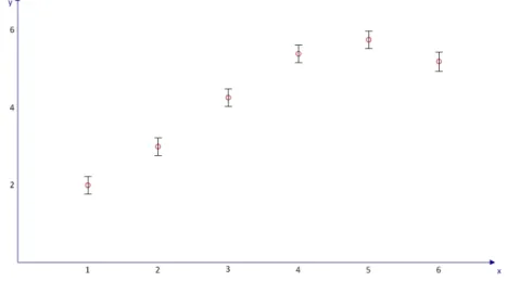
Suppose we have a sample dataset with 5 inputs and their observed output values y, as shown in Table 3.1. The problem in regression is to predict the output value y for the new input value x=6 as shown in Figure 3.3. Each observation has a noise value as illustrated by the error bars. Similarly we should estimate the error bars (the confidence interval) for the predicted value in regression analysis.
Table 3.1: Sample dataset for regression.
x 1 2 3 4 5 6
y 2.0 3.0 4.25 5.5 5.75 ?
Figure 3.3: A set of sample training data points with one test data point whose target value is unknown.
Inputs can be of single dimension or multiple dimensions. In general, it is a vector and the output is a single scalar value.
As mentioned above, statistical inference can be performed by learning a function from the sample training dataset with different input-output patterns. However the accuracy of inference is solely based on the method we choose for the underlying function that maps the input to the correct outputs.
3.5
Gaussian Process Regression
In this section we look at how Gaussian process can be used to perform regression. Before seeing any data, first we have to assume the underlying function (Gaussian prior) and select a proper covariance function. However, this selection of a proper kernel should be done in accordance with the characteristics of the data considered. Then Gaussian process specified by the respective kernel function will produce a distribution of random functions.
After the training data points are introduced , it selects the best matching functions from the distribution that pass through or pass closely to the given data points. In this way it finds the best possible set of functions from the Gaussian prior. For better forecasting accuracy, GP requires adequate number of training samples.
However, the selection of the best functions solely depend on the choice of kernel function and its parameters. Although GP is a non parametric model, the kernel function is associated with some parameters such as signal variance and length-scale parameter. These parameters should be set properly for better learning experience.
Suppose we are given a training datasetD={(xi, yi)|i= 1,2, ..., n}with noisy observations,
and we need to predict the target value y∗ for the new input value x∗. The problem is to
learn a function from the dataset, which involves an assumed Gaussian prior of functions. In fact, the observations and the underlying function f values are not the same due to the noisy measurements of the observations. Therefore the targets can be represented as:
y=f(x) +ε, (3.11)
with the assumption of a Gaussian noise model represented byε∼N(0, σn2). The underlying function f is approximated by a Gaussian process with zero mean function and a covariance function. The most commonly used covariance function is the Squared Exponential covariance function. Using this function we can express equation 3.7 as,
f(x)∼GP(0, k(x,x0)) (3.12)
k(x, x0) =σf2exp[(x−x
0)2
2l2 ] (3.13)
According to equation 3.11, the actual observations (i.e y) can be specified by adding the noise model to the underlying function defined by equation 3.12. Then the covariance function related to the target values y, denoted as cov(x, x0), can be given by:
cov(x, x0) =k(x, x0) +σ2nδ(x, x0) (3.14) whereδ(x, x0) is the Kronecker delta function which is equal to 1 iffx=x0 and 0 otherwise. Using the kernel function, the correlation between each and every training data point can be measured. The matrix generated with each of these covariance value as elements is known as theCovariance matrix and denoted by K.
K =
cov(x1, x1) cov(x1, x2) · · · cov(x1, xn) cov(x2, x1) cov(x2, x2) · · · cov(x2, xn)
..
. ... . .. ...
cov(xn, x1) cov(xn, x2) · · · cov(xn, xn)
(3.15)
The corresponding covariance matrix between the training data points and the test data points is given byK∗:
K∗ =
cov(x∗, x1) cov(x∗, x2) · · · cov(x∗, xn)
(3.16)
K∗∗ specifies the covariance matrix between the test data points itself.
K∗∗=cov(x∗, x∗) (3.17)
The joint distribution of the observations y and the predictions y∗, has been found as a
multivariate Gaussian distribution [28]:
y y∗ ∼N 0, K K∗T K∗ K∗∗ (3.18)
In fact, the actual prediction that we are interested in is given by the conditional distribution of y∗ given y
y∗|y∼N(K∗K−1y, K∗∗−K∗K−1K∗T) (3.19)
This particular distribution is known as the posterior Gaussian distribution. According to Rasmussen and Williams [26], for any Gaussian posterior, the mean of the posterior distribution is called as theMaximum a Posteriori (MAP) value, which is the best estimate for the variable considered. In equation 3.19 the actual prediction y∗ is its mean, which is the MAP estimate:
¯
y∗ =K∗K−1y (3.20)
The variance of the estimation is given by
var(y∗) =K∗∗−K∗K−1K∗T (3.21)
The variance is used to calculate the 95% confidence interval of the prediction as±1.96pvar(y∗),
which is approximately two times the standard deviation of the posterior distribution.
Now, let us apply these equations to the example shown in 3.3 and forecast the value of y atx∗=6 using Gaussian process. Suppose σf=3.35, l=2.95 andσn=0.08. Using these value we
can calculate the covariance matricesK,K∗ andK∗∗ as follows:
K= 11.27 10.63 8.95 6.72 4.49 10.63 11.27 10.63 8.95 6.72 8.95 10.63 11.27 10.63 8.95 6.72 8.95 10.63 11.27 10.63 4.49 6.72 8.95 10.63 11.27 (3.22)
K∗ =
2.68 4.49 6.72 8.95 10.63 (3.23)
K∗∗= 11.27 (3.24)
Applying these values to equations 3.20 and 3.21, we get the prediction of y at x∗=6 and
the variance of the prediction.
¯
y∗ = 5.06 (3.25)
var(y∗) = 0.14 (3.26)
Now we can visually illustrate the results, with the predicted value and the 95% confidence interval as shown in Figure 3.4.
Figure 3.4: A set of sample training data points with the predicted target value of the test data point.
Equations 3.20 and 3.21 has a considerable computational issue because of the inverse op-eration of K of sizen2 [19]. Here n is the number of observations. Therefore, the complexity of
Gaussian process isO(n3). However it can be reduced to a complexity ofO(nm2) by selecting an active subset of columns of K. Here m is the rank of the matrix approximation [19]. Also cholesky decomposition can be used to factorize K, to get a numerically stable approximation [19].
3.5.1 Selection of Hyperparameters
The noise variance σ2n, and the parameters in the kernel function are taken as the free hyper-parameters in Gaussian process. This is represented by the vectorθ:
θ={l, σ2f, σ2n} (3.27)
wherelis the characteristic length scale,σ2f is the signal variance andσ2nis the noise variance. In Gaussian Process Regression(GPR) , these three parameters are obtained by learning the data. In general, it uses Bayesian model to infer these parameters. This method is known as
marginal likelihood maximization method. According to the Bayes rule, we can represent the posterior probability of the parameters as follows:
p(θ|X, y) = p(y|X, θ)p(θ)
p(y|X) (3.28)
p(y|X, θ) is the marginal likelihood which is to be maximized, andp(θ) is the prior probability of the parameters.
The marginal likelihood can be calculated by marginalizing the integral of the likelihood and the Gaussian prior, over the latent function f.
p(y|X, θ) =
Z
p(y|f, X)p(f|X)df (3.29)
Both p(y|f, X) and p(f|X) follow Gaussian distributions. The log value of the marginal likelihood gives the parameters which has been found as [26]:
L(θ) = logp(y|X, θ) =−1 2y TK−1y−1 2log|K| − n 2log2π (3.30)
The first term −1 2y
TK−1y represents the data-fit,which is the only term that contains the
observed target values. The second term is the complexity penalty and the last term is a normalization constant.
Traditional Approaches of Electricity
Consumption Forecasting
In this thesis, results of Gaussian process are compared with the traditional techniques used for electricity consumption forecasting. We have selected two such traditional techniques : Artificial Neural Networks and Linear regression. The purpose of this chapter is to give the theoretical foundations of both ANN and linear regression. Section 4.1 introduces the concepts of ANN including its variants back-propagation and multiple back-propagation. Section 4.2 outlines the basics of linear regression and multiple linear regression explaining how regression is performed under different input variables.
4.1
Artificial Neural Networks
Artificial neural networks have been used for forecasting electricity consumption as we men-tioned in chapter 1 and 2. In this section we go deeply into the theoretical aspects of ANN, and back-propagation based ANN which we use to test our dataset, to compare the results with Gaussian processes.
4.1.1 Introduction to ANN
The concept of ANN arises from the knowledge of the biological nervous systems [29]. The nervous system is constructed by a number of structural constituents known asneurons, which are connected to each other by links. This network of neurons connected through links, is referred to as aneural network.
A neuron is defined by Patterson [29] as follows:
Figure 4.1: A typical neuron in a biological nervous system. [Source:http://www.mindcreators.com/NeuronBasics.htm]
and responds by generating electrical impulses that are transmitted to other neurons of effector cells.
There are about 1010 to 1012 neurons in the human nervous system [29], which contains trillions of interconnections between them that makes it a highly complex system. Basic com-ponents of a typical neuron cell is illustrated in Figure 4.1.
The cell body is known as the Soma. A neuron cell has an input side and an output side. The input side is the one which is named as dendrites in the figure. Dendrites are connecting the outputs from the other neurons to this neuron through synapses. There are a number of various synaptic connections to the neuron from which it can receive input signals. The outputs are carried through the axon to other neurons (through dendrites) or directly to effector organs such as muscles and glands.
Neurons can be categorized into three as input, output and intermediate neurons. In the human body, input and output neurons constitute 10% of the neurons and the remaining 90% store informations and other signal transformations [29].
These concepts of neurons and biological nervous system have led scientists to develop the artificial neural networks.
4.1.2 Back-Propagation Neural Networks
Back Propagation Neural Network(BPNN) , one form of ANN, is a non parametric statistical modelling technique, which is used in regression. It is considered by Smith [30] as the only form of neural network which has produced a number of commercial applications. It is a feed-forward network which has the ability to propagate prediction error, back to the network as a feedback and improve its results.
In its simplest form, a BPNN basically composed of three layers of neurons(nodes) - input layer, hidden layer and output layer. Figure 4.2 depicts a typical feed-forward network with these three layers. It consist of 4 input nodes (representing four independent variables), 3 hidden nodes (which performs the basic calculations) and 2 output nodes(representing two
Figure 4.2: A typical feed-forward network used for back-propagation
output variables).
Each layer in the BPNN is associated with a particular functionality. Similar to the biological nervous system, the input nodes in the BPNN receives input values. But in this case, they receive the values of the independent variables used in the training process. If there are n
number of variables in the feature vector, the network requires n input nodes in the input layer to accommodate the corresponding variables. The output nodes represent the dependant variables that needs to be estimated by the network. They output the estimated values of the dependant variables. Hidden layer is the intermediate layer which does the basic inner workings of the neural network, and also got its name hidden as it acts as a black box to the outside environment.
Every node in each layer is connected to the next layer by links ,which is analogous to the synaptic connections and dendrites in the biological nervous system. However, note that, there is no process likeback-propagation in actual human brain [30].
Now we should pay our attention as to how BPNN estimates the values of the output variables given the training set of input-output pairs. Back-propagation involves two types of passes: aforward pass, which is referred to as a mapping from inputs to outputs, and abackward pass, which is referred to as the learning of the network.
In forward pass, a relationship, which is a mathematical equation, is generated (called the
mapping function) between the input nodes and the output nodes across different connections in the network. Each connection between neurons has a certain strength which is termed as the weight between the two neurons. These weights play an important role in BPNN as they change their values in order to obtain better estimates.
The mapping function is built by using some standard functions. These functions used in the neural networks is so flexible that it can be configured to be close to any target function [30]. It
-4 -2 2 4 x 0.2 0.4 0.6 0.8 1.0 gHxL
Figure 4.3: The logistic function which is one type of sigmoid functions.
achieves this flexibility from the weights of the equation. In general, this function is constructed basically by the sigmoid functions.
A sigmoid function takes the S shape. It should be bounded (i.e has an upper limit and a lower limit), monotonically increasing and differentiable. The most commonly used sigmoid function used in neural networks is thelogistic function [30] depicted in equation 4.1.
g(x) = 1
1 +e−x (4.1)
Figure 4.3 illustrates the curve for the logistic function between the interval -4 and +4. Now we must look at how the mapping function is constructed in a back-propagation neural network. Suppose the network has two input nodes, two hidden nodes and one output node as shown in Figure 4.4. x1 and x2 are the two input values. wij are the weights of each link from
the input neurons and the hidden neurons where i = 1,2 and j = 1,2 for Figure 4.4. These weights are stored in the memory of hidden neurons. In addition to that, each hidden neuron stores a bias values which are shown as b1 and b2 in the figure. u1 and u2 are calculated in the
hidden layer as a weighted sum of each input value as shown in equation 4.2 and 4.3.
u1 =b1+x1w11+x2w12 (4.2)
u2 =b2+x1w21+x2w22 (4.3)
Instead of outputtingu1 andu2, the hidden neurons output the logistic values of them as the
inputs to the next layer. Therefore the two outputsy1 and y2 can be expressed as in equation
Figure 4.4: A BPNN with weights and bias values. Neurons are represented by circles and bias by triangles. y1 = g(u1) = g(b1+x1w11+x2w12) = 1 1 +e−(b1+x1w11+x2w12) (4.4) and y2 = 1 1 +e−(b2+x1w21+x2w22) (4.5)
Now y1 and y2 become the inputs to the output node o. The output node also perform a
similar calculation to generate the final output valuez. Similar to the hidden nodes, the output node also has a bias valueband weights for each connection link (i.ewo1 and wo2). The output
valuez is given by
z = g(o)
= 1
1 +e−o (4.6)
where o is the weighted sum of the outputs coming from the hidden layer
o=b+y1wo1+y2wo2 (4.7)
can be given as [30]: zk=g(ok), k= 1, ..., K (4.8) where, ok=bk+ J X j=1 wjkyj (4.9)
In general, if we assume a multilayer network with n input nodes, J hidden nodes and one output node. The equation 4.2 is generalized to
uj =bj+ n
X
i=1
xiwji, j= 1, ..., J (4.10)
and the generalized output from the hidden nodes can be calculated using the logistic func-tion. yj = g(uj) j = 1, ..., J = g bj+ n X i=1 xiwji ! (4.11)
The final estimated output can be found by applying the weighted sum and subsequently applying the activation function to it as follows.
o=b+
J
X
j=1
yjwoj (4.12)
z = g(o) = g b+ J X j=1 yjwoj = g b+ J X j=1 " g bj + n X i=1 xiwji ! woj # (4.13)
After the forward-pass is finished and the output is calculated, the backward-pass com-mences. This is also known as the learning process. The learning here refers to adjusting the weights we discussed above such that the mean squared error between the estimated and target values gets smaller. The method used to achieve this is gradient descent. The adjustment to the weights is done in the backward process by propagating the mean squared error from the output side to the hidden nodes. Therefore this method gets the name back-propagation . The training examples are feed to the network and possible output pattern is generated in forward pass. Then the estimated output pattern is compared with the desired output pattern and the difference is propagated in backward pass indicating the direction in which the correct adjust-ments should be made. In this way the weights between the hidden layer and the output layer are adjusted. This process is repeated a considerable number of iterations (known as epochs) until the total average error of the outputs converges to a minimum value.
4.1.3 Multiple Back-Propagation
In this thesis, we use the MBP Software1 developed by Lopes and Ribeiro [2], to test for neural networks. In [2] they describe about Multiple Back-Propagation (MBP), which is a generalization of the BP algorithm.
Here, a Multiple Feed-Forward network is used, which is obtained by integrating two FF networks : Main network and space network as shown in Figure 4.5.
The output of selective activation neurons in the main network is given by [2]:
ypk=mpkFk( N
X
j=1
wjkyjp+θk), (4.14)
where ykp is the output of neuron k for pattern p, mpk the importance of the neuron for the output of the network,Fk the neuron activation function,θk the bias andwjk the weight of the
connection between neuron j and k. The main network can calculate its output only after the space network outputs are calculated. In the learning pass, the weights of both the networks
Figure 4.5: A Multiple feed-forward network. Hidden and output neurons are represented by circles, input neurons by squares, and bias by triangles [2].
should be adjusted. For more information about MBP networks see [2, 31, 32], and in Appendix A we have included some screen shots of the tool used for forecasting using MBP network.
4.2
Linear Regression
Linear regression is a common regression technique used in most inferring problems. Unlike neural networks, it lacks the ability to capture non-linear relationships between variables. How-ever it is considered as one of the methods, which is easy to fit and highly scalable [19]. In the following sections we will describe basic theoretical aspects of linear regression and multi-ple linear regression and how we can use it to infer predictors using IBM SPSS ® Statistics software.
4.2.1 Statistical Significance
Before moving into the prediction, lets consider about the significance value which is mostly used in linear regression. It is also termed as significance or probability which is denoted by the letter p. The likelihood that a particular outcome may occur by chance is given by the p value. It can be used to identify whether two or more variables are correlated to each other signifi-cantly. So we should always try to find a very smaller p value for valid results. Social scientists have accepted that a p value less than 0.05 is statistically a significant correlation [33].
0 1 2 3 4 5 6 0 1 2 3 4 5 6 x y
Figure 4.6: Scatter plot of the sample dataset.
4.2.2 Linear Regression
Linear regression analysis is a way of testing hypothesis concerning the relationship between two numerical variables and a way of estimating the specific nature of such relationships [34]. The relationship is expressed in the form of an equation or a model connecting the dependant variable and one or more independent variables depending on the problem of interest. The method of least squares is used most frequently in fitting a line in linear regression.
The simplest relationship between an independent variable x and a dependant variabley is represented as
y=β0+β1x+ (4.15)
where β0 is the intercept and β1 is the slope. The random error term is given by which
should be normally distributed with 0 mean and at each possible value of x, the variance of|xi
should be constant and it should be independent of the other errors [34]. Normally we examine the residuals which are the differences between the observed values (y) and the estimated values to approximate this error term.
These unknowns have to be found using the samples in the training dataset. Lets consider the sample dataset found in Table 3.1 in chapter 3, which has an independent variable x and dependant variabley as shown in Figure 4.6.
SPSS generates four tables in linear regression analysis. Table of variables in the regression equation, amodel summary, an ANOVA table, and atable of coefficients.
Table 4.1: Variables table.
Model Variables Entered Variables Removed Method
1 x Enter
A variables table with only one independent variable is shown in Table 4.1. We can have multiple linear regression models if we have multiple variables based on the variables in the Entered and Removed columns. However in this case there is only one model due to the availability of one independent variable.
Table 4.2: Model summary table.
Model R R Square Adjusted R Square Std. Error of the Estimate
1 .984 .969 .958 .32914
The model summary table shown in Table 4.2 illustrates the goodness of fit in regression. Here, R is the correlation coefficient which ranges from -1 to +1 and R2 is the coefficient of determination which is the squared of R. If R2 is equal to 1, then it is a perfect fit. The value in the given table (i.e 0.969) is very close to one, meaning that the points in the dataset are experiencing a very good linear relationship. The adjusted R square value is a more better value than R square value which can be used for population estimates specially in multiple regression. The third table is the ANOVA table. ANOVA is used to compare three or more means to one another. For a single independent variable it is called one-way ANOVA [34].
Table 4.3: ANOVA table.
Model Sum of Squares df Mean Square F Sig.
1 Regression 10.000 1 10.000 92.308 .002
Residual .325 3 .108
Total 10.325 4
The Sig value is also known as the P-value and, if it is less than 0.05 we say the ANOVA is significant( F value is significant) and it can be concluded that there is a regression in the model. The F value in the table is known as the Levene statistic. In Table 4.3, the p value is less than .05, and therefore we can conclude that the two variables are statistically significant.
0 1 2 3 4 5 6 0 1 2 3 4 5 6 7 x y
Figure 4.7: Fitted line for the sample dataset.
Table 4.4: Coefficients table.
Model Unstandardised Coefficients Standardized Coefficients t Sig.
B Std.Error Beta
1 (Constant) 1.100 .345 3.187 .050
x 1.000 .104 .984 9.608 .002
The last table is the table of coefficients. We know that β0 and β1 are the coefficients in
equation 4.15. The first value in column B (i.e 1.100) is the intercept β0 and the second value
1.000 is the slope β1. If we consider the t value and the significant value for the slope, the
significance value is less than 0.05 meaning that there is a statistically significant relationship between x and y.
Using thes information we can interpret equation 4.15 as follows for the considered dataset.
y= 1.1 +x+ (4.16)
The fitted line for the above discussed dataset could be illustrated as shown in Figure 4.7. Now we can estimate the output of the target variable when x=6, i.e y=7.1.
But now we should pay our attention to the error term (or disturbance) of the fitted line. For this, we have to look at Table 4.2. The standard error of the estimate .329, is a measure of the variability of the random error. This can be used to calculate the 95% confidence interval by multiplying by two. This can be considered as the residual error term for the regression line. Therefore our estimate for y should be as follows:
Figure 4.8: The normal P-P plot of regression, which is used for residual analysis.
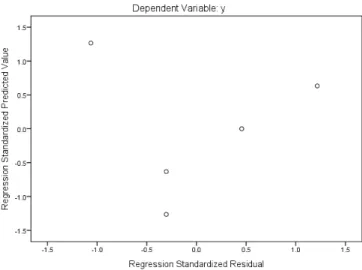
Figure 4.9: Graph of standardized predicted value versus standardized residual value, which is used for residual analysis.
y= 7.1±.658
To find out the validity of the first assumption of the residuals (i.e normality) we look at the normal probability plot as shown in Figure 4.8.
The assumption of equal variances can be identified by the scattered plot of the standardized residuals versus the standardized fitted values. [34]. This is illustrated in Figure 4.9.