Roffo, G., Melzi, S., Castellani, U., Vinciarelli, A. and Cristani, M. (2020) Infinite
feature selection: a graph-based feature filtering approach. IEEE Transactions on Pattern
Analysis and Machine Intelligence, (doi: 10.1109/TPAMI.2020.3002843).
There may be differences between this version and the published version. You are
advised to consult the publisher’s version if you wish to cite from it.
http://eprints.gla.ac.uk/218830/
Deposited on: 24 June 2020
Enlighten – Research publications by members of the University of Glasgow
http://eprints.gla.ac.uk
Infinite Feature Selection:
a Graph-based Feature Filtering Approach
Giorgio Roffo, Simone Melzi,
Member, IEEE
, Umberto Castellani,
Alessandro Vinciarelli,
Member, IEEE
and Marco Cristani,
Member, IEEE
Abstract—– We propose a filtering feature selection framework that considers a subset of features as a path in a graph, where a node is a feature and an edge indicates pairwise (customizable) relations among features, dealing with relevance and redundancy principles. By two different interpretations (exploiting properties of power series of matrices and relying on Markov chains fundamentals) we can evaluate the values of paths (i.e., feature subsets) of arbitrary lengths, eventually go to infinite, from which we dub our framework
Infinite Feature Selection(Inf-FS). Going to infinite allows to constrain the computational complexity of the selection process, and to rank the features in an elegant way, that is, considering the value of any path (subset) containing a particular feature. We also propose a simple unsupervised strategy to cut the ranking, so providing the subset of features to keep. In the experiments, we analyze diverse setups with heterogeneous features, for a total of 11 benchmarks, comparing against 18 widely-know yet effective comparative approaches. The results show that Inf-FS behaves better in almost any situation, that is, when the number of features to keep are fixed a priori, or when the decision of the subset cardinality is part of the process.–
Index Terms—Feature selection, filter methods, Markov chains.
F
1
INTRODUCTION
O
VERthe last few decades, successful approaches to machinelearning problems have been based initially on hand-crafted features (e.g., SIFT and HOG-like [1], [2], [3], [4],
dictionary-based [5]) that evolved into automatically learned ones with the
diffusion of deep learning models [6], [7], [8]. Through these
advancements, feature selection (FS) still remains an active and growing research area that enables both dimensionality reduction and data interpretability, looking for features which are relevant and not redundant [9], [10], [11].
In this paper we introduce a fast graph-based feature filtering approach that ranks and selects features by considering the pos-sible subsets of features as paths on a graph, and works in an unsupervised or supervised setup.
Our framework is composed by three main steps. In the first step, an undirected fully-connected weighted graph is built,
where the node ~vi, 1 ≤ i ≤ n, corresponds to the feature
fi, and each edge connecting~vi to~vj has associated a weight,
or value, modeling the expectation that features fi and fj are
relevant and not redundant. The weight comes from customizable pairwise relations among feature distributions, which can be easily crafted by the user, and, as a future perspective, learned directly from data. Here we present two instances of pairwise relations:
one exploiting class information (Inf-FSS), the other one being
completely agnostic (Inf-FSU).
In the second step, the weighted adjacency matrix associated to the graph is employed to assess the value of each feature (i.e., a node in the graph) while considering possible subsets of features (i.e., subsets of nodes) as they were paths of variable length. Two
• G. Roffo and A. Vinciarelli are with the School of Computing Science, University of Glasgow, Glasgow, UK.
• M. Cristani, S. Melzi and U. Castellani are with the Department of Computer Science, University of Verona, Verona, Italy.
Manuscript received August 5, 2019.
interpretations can be exploited: one comes from the properties of power series of matrices, the other one from the concept of absorbing Markov chain. In both the cases, we compute a vector
which at the i-th entry expresses the value (or probability) of
having a particular feature in a subset of any length, summing for all the possible lengths, until infinite. Going to infinite allows
us to reduce the computational complexity from O(n3lT) (n
features,lpath length,Tsamples) toO(n3T). For this reason, we
dubbed our approachInfinite Feature selection (Inf-FS). Ranking
the values of the “infinite” vector gives the ordered importance of the features.
In the third step, a threshold over the ranking is automatically selected by clustering over the ranked value. The rationale is to individuate at least two distributions, one which contains the features to keep with higher value, the other the ones to discard.
The proposed framework is compared against18comparative
approaches of feature selection, with the goal of feeding the selected features into an SVM classifier.
As for the datasets, we selected 11 publicly available bench-marks to deal with diverse FS scenarios and challenges. In particular we consider five DNA microarray datasets for
can-cer classification (Colon [12], Lymphoma [13], Leukemia [13],
Lung [14], Prostate [15]), handwritten character recognition
(GINA [16]), general classification tasks from the NIPS feature
selection challenge (MADELON, GISETTE [17], DEXTER [18]),
and two object recognition datasets with convolutional neural
networks (CNNs) features (PASCAL VOC 2007 [19] and CalTech
101 [20]).
One of the most interesting aspects shown in the experiments is the flexibility of Inf-FS, both in its unsupervised and super-vised version: independently on the scenario (small-sample+high dimensional, unbalanced classes, severe interclass overlap, noise) Inf-FS overcomes the competitors, and if not, it gives the sec-ond or third best performance, promoting itself as all-purpose feature selection strategy. Another important achievement is that
the automatic thresholding individuates those features capable of providing convincing performance on any given dataset. Finally, Inf-FS operates also on neural features, improving relevance and diminishing redundancy over cues that have been the state of the art until very few years ago [21].
The proposed framework generalizes the previously published
Infinite Feature Selection (Inf-FS) [22], [23] presented as an unsupervised filtering approach, explained by algebraic motivations. Here we introduce a supervised counterpart and a strategy to select a subset of features, supported by a novel alternative way to explain the Inf-FS thanks to Markov chains fundamentals.
The rest of the paper is organized as follows: Sec.2illustrates the related literature, including the comparative approaches we
consider in this study. Sec. 3 introduces our approach showing
how the fully-connected graph is built for both the unsupervised
and supervised variants. Sec.3.5connects the proposed approach
to the absorbing Markov chain framework, deriving the subset se-lection strategy. Extensive experiments are reported in Sec.4, and, finally, in Sec.5, conclusions are given and future perspectives are envisaged.
2
STATE
OF
THE
ART
Feature selection (FS) algorithms are partitioned into three main
classes [24], [25]: filters, wrappers and embedded methods.
Filter methods make use of the intrinsic properties of the data
(e.g., correlation, variance, locality, information gain, or other
statistics) to evaluate the value of a feature. In contrast,wrapper
methods assign an importance score to each feature based on the performance of a predictor, which is considered as a black
box [26]. Last, embedded methods include the feature selection
process as part of an internal regression model aimed at estimating the relationships among variables. The outcome of this process is also the solution to the feature selection problem (e.g., least square
regression (LSR) [10], least absolute shrinkage and selection
operator (LASSO) [27]).
Inf-FS belongs to the filter approaches, since it deals with the sole properties of the data, without relying on a specific predictor. This ensures a wider applicability, but at the same time does not exploit the potentialities of a particular classifier.
Within each of the above families of algorithms, FS techniques
can be further classified into two sub-categories, unsupervised
andsupervised, depending on the use of class-label information in the selection process. In this paper we offer one specific example of Inf-FS for both the cases, showing the portability of the framework.
Most of the FS algorithms are sorting algorithms, that, after having evaluated the feature set, the output is a sorted list of features. The output is then used to decide which features to keep (subset selection). Subset selection is commonly performed by cross-validation strategies in a classification scenario with the classifier exploiting the candidate features on some validation data [25].
The section overviews the three families of FS methods (filters, wrappers and embedded methods) specifying when they are unsu-pervised or suunsu-pervised, discussing their strengths and weakness.
2.1 Filter methods
2.1.1 Unsupervised approaches
In unsupervised scenarios, methods are mainly based on locality preserving principia found by clustering (data from the same cluster are often close to each other). The Laplacian Score (LS) for
FS [28] evaluates the value of features by considering their
ten-dency of preserving spatial relationships, that is, samples assigned to a particular group are at a shorter distance to each other than to those in other groups. Thus, LS constructs a nearest neighbor graph and ranks high those features that are consistent with
Gaussian Laplacian matrix [28]. Similarly, in the multi-cluster
feature selection approach (MCFS) [29], features are selected
based on spectral analysis and solving a sparse regression problem, encouraging the formation of compact clusters. Local learning
clustering (LLCFS) method [9] is a kernel learning method that
weights features and exploits the weights to regularize the clus-tering. Noteworthy, uninformative features are left out before the clustering.
These solutions, included in the experiments, are computation-ally expensive since rely on clustering. In contrast, our approach is faster since it only uses intrinsic properties of the data.
2.1.2 Supervised approaches
A standard two-class filter method is Relief and its multi-class
extensionRelief-F[30]. In general, the strategy evaluates feature value differences between nearest neighbor pairs and scores fea-tures according to how well they contribute to the overall class separation. One common criticism of relief is that it leads to
the selection of a redundant subset (i.e., features expressing the
same information), since it is not controlling feature correlation. A solution is given by the minimum Redundancy and Maximum
Relevancy (mRMR) algorithm [31], minimizing the redundancy
and maximizing the relevance of the set of features (i.e., relevant features are tightly connected to classes). This is obtained by maximizing the joint mutual information (using Parzen Gaussian
windows [32]) between the values of a given feature and the
membership to a particular class. mRMR suffers from an
expen-sive computational cost (i.e., O(n2T3)where n the number of
features andT the number of samples [31]), which makes this
algorithm not suitable for massive highly-dimensional data [25].
Another weakness of mRMR comes with the approximation of the mutual information, which is inaccurate when the number of training samples is small [32]. A practical yet faster filter approach is theFisher score[33], which assigns scores to features according to the ratio of inter-class separation and intra-class variance while evaluating each feature independently.
Several other algorithms employ mutual information (MI) to assess features usefulness. The standard MI method for feature
selection proposed in [34] estimates the mutual information
be-tween feature distributions and class labels. All the features are evaluated independently, one by one, obtaining a score that the MI method uses to rank all the features set. The recent
Max-Relevance and Max-Independence (MRI) [35] introduces an
additional constraint: relevancy. MRI does maximize the inde-pendent classification information while minimizes the
redun-dancy between features. Other MI-based [36] approaches, such as
CIFE [37], MIFS [38] and ICAP [39], quantify the redundancy (or dependency) among the set of feature distributions (considered as random variables) by proposing slightly different variations of the objective function. i.e., the conditional likelihood of the training
labels. Similarly, the joint mutual information (JMI) [40] and
conditional mutual information (CMIM) [41] for feature selection
can be included into this group. The common assumption behind all these methods is that a less dependency among features can af-fect the classification performance and enhance the discriminative ability of the entire feature subset.
The Inf-FS framework is attractive since, in its computation of the weighted adjacency matrix, allows to include inter/intra class reasoning, but is independent from it: in fact, the supervised
Inf-FSS proposed in this paper makes use of a fast computation of
the mutual information and Fisher criterion, but is not a necessary requirement. Especially in the case of large number of samples, mutual information may be dropped in favor of other, faster, feature analysis. Another difference with Inf-FS is that the MI-based approaches take into account pairwise (feature-class label)
dependencies, while our approach extends the2-nd order ton-th
order by considering subsets of features as paths on a graph. Recently, other graph-based approaches have been proposed
such as the eigenvector centrality (ECFS) [42], [43] and the
infinite latent feature selection (ILFS) [22], which is an extension
of the unsupervised Inf-FSU. The ECFS ranks features according
to a centrality measure over the graph of features (eigenvector centrality), and should be considered a lighter version of Inf-FSU,
with the mathematical difference explained in Sec.3). In ILFS the
features are grouped into token by probabilistic latent semantic analysis (PLSA), which in practice learns the weights of the adjacency graph of Inf-FS as to provide better class separability. Instead, our framework requires to craft the weights manually. Despite the experiments show our approach overcoming ILFS, we think learning the weights is a convenient direction, which we are interested at the present moment.
Summarizing, some advantages of using filter methods are:
• faster than wrapper and embedded methods,
• scalable,
• classifier independent (better generalization),
On the other hand, disadvantages are related to a general lower performance, being independent on the specific classifier.
2.2 Wrapper approaches
2.2.1 Unsupervised approaches
In the dependence-guided unsupervised feature selection
(DGUFS) [44], graph-based clustering is adopted as clustering
approach. DGUFS iteratively performs feature selection by op-timizing two terms: one term increases the dependence among samples of the same cluster (i.e., assign samples to clusters), while the other term favours those features that maximize the dependence between samples and the assigned cluster labels. This approach shows to be prone to local minima.
The feature selection with adaptive structure learning
(FSASL) [45] is an iterative approach that captures the global
structure of data within a sparse representation framework, where the reconstruction coefficient is learned from the selected features. Its main drawback is the high computational complexity (see Table1).
Finally, the unsupervised feature selection with ordinal locality
(UFSOL) is proposed in [46]. UFSOL is a clustering-based
approach that preserves the relative neighborhood proximities of the samples and contributes to distance-based clustering.
Similarly to our approach, these last three methods methods estimate inter-relationships among features, but in these cases
the estimations are intermediate steps of iterative clustering pro-cedures that make them computationally expensive and prone to local minima. Conversely, Inf-FS does not suffer from local minima since it is one-shot, deterministic.
2.2.2 Supervised approaches
The support vector machine with recursive feature elimination
(RFE) [47] is a popular wrapper method that eliminates useless
features in a sequential, backward fashion, ranking high a feature if it actively separates the samples using a linear SVM. However, the performance of the RFE becomes unstable at some values of the filter-out factor (i.e., the number of features eliminated in
each iteration) [48]. To overcome this weakness many different
variants of RFE have been proposed, where the initial feature subset is selected using several SVM models with different filter-out factors, and in the second stage, features are selected by eliminating one feature at each iteration. For example, the sample
weighting version calledSW SVM-RFE[49], gives more weight to
those samples that are close to the separating hyperplane. Another
extension of the RFE method is the Ensemble SVM-RFE [49]
that aggregates the results of several SVM-RFE selectors applied to randomized training data and has been empirically shown to be stronger than its original version. Finally, a slightly different
approach called recursive cluster elimination (RCE) [50] has been
introduce to overcome the RFE instability and provide improved classification accuracy. RCE is a backward elimination algorithm that combines K-means to identify correlated clusters of features to identify and rank features for classification.
Some advantages of using wrapper methods are:
• they find specific features for a particular classifier better than filters,
• they consider the dependence among features (multivariate
solutions),
• higher classification accuracy than filters.
The disadvantages are their tendency to be highly classifier specific (different classifiers bring to diverse features) and their computational requirements. On the contrary, Inf-FS is classifier agnostic, focusing only on intrinsic properties of data and their labels. We omit the RFE-X approaches in the experiments since
they have been already shown to be inferior to Inf-FS in [23].
2.3 Embedded methods
Finally, embedded methods include the selection process as part of an internal regression model, and the overall ranking process is less prone to overfitting than wrappers (e.g., L1, LASSO regularization, decision tree). In contrast to wrapper methods, which assess subsets of features according to their usefulness to a given predictor, embedded methods proceed more efficiently to the solution by directly optimizing an objective function that involves two constraints: the goodness of fit of the statistical model and a penalty for selecting a large number of features [51].
An example of unsupervised embedded method is the L2,
1-norm regularized discriminative feature selection for unsupervised
learning (UDFS) [52]. UDFS optimizes an objective function
representing a L2,1-norm regularized minimization problem with
orthogonal and locality preserving constraints [53] so that it
simultaneously exploits discriminative information and feature correlations. However, such optimization problems are difficult to solve due to the non-smooth objective function and non-convex constraints [53].
2.3.1 Supervised approaches
In supervised learning scenarios, the support vector machine intervenes in many approaches. The Feature Selection concaVe
(FSV) [11] generates a separating plane by minimizing a weighted
sum of distances of misclassified points to the two margin planes, minimizing the number of dimensions of the space used to determine the separating plane, and at the same time, maximizing the distance between the two margin planes. Another SVM-based feature selection approach minimizes the 0-norm with SVMs
(L0) [54]. Indeed, L0 is a variant of the standard SVM algorithm,
obtained by an iterative multiplicative rescaling of the training data. Feature selection is solved by minimizing the zero-norm in a single optimization, resulting in a minimization of the training errors and maintaining sparsity in the solution. After training, features associated with higher scores are those that contribute to the model construction and its performance the most. Least square regression (LSR) and several variants of LSR have been applied
as a feature selection tool. The LASSO [27] regression approach
minimizes the squared prediction error while maintaining the sum of the absolute values of the model parameters smaller than a fixed value. Feature selection is a consequence of this process when all the variables that still have non-zero coefficients are selected to be part of the model. For classification, LASSO is modified by
exploiting a hinge loss (LASSOh) which penalizes linearly with
respect to the correct classification labels [55]. More recently,
unhinged losses have shown to be more robust against biased
estimates [56] which are a known issue of LASSO (LASSOu).
Since in the experiments we evaluate the goodness of the features kept by the selection approaches with simple linear support vector machines (as LASSO is), we consider as comparative approaches
both LASSOhand LASSOu.
Another way to deal with the bias issue of LASSO lies on the use of non convex optimization strategies, as the ones of the hard-thresholding approaches. Under the hypotheses of strong restricted convexity/smoothness of the function to be minimized, recent hard
thresholding approaches are GraHTP [57], [58] and NHTP [59],
the latter included as comparative approach.
Advantages and disadvantages of using embedded methods are similar to those listed for wrappers (they are tightly coupled to the solver which separates the data), however, a further advantage that the embedding process brings in is to be less prone to over-fitting than wrappers. In any case, Inf-FS is conceptually different, being
a filter which prepares the data to a subsequent, disconnected
classification step. This makes it more versatile and customizable.
3
OUR
APPROACH
We propose two different versions of Inf-FS: the unsupervised
Inf-FSU and the supervised Inf-FSS. In both the cases, we build
upon a weighted undirected fully-connected graphG = (V, E)
with node setV = {~v1, ..., ~vn}representing a set of nfeature
distributionsF ={f1, ..., fn}, and edge setEmodeling relations
among pairs of nodes (i.e., relations among distributions). In the
following, the termsfeatureandfeature distributionwill be used
interchangeably.
Let us represent Gwith its adjacency matrixA, where each
of its elementsA(i, j),1 ≤i, j≤n, models the confidence that featuresfiandfj (the nodesv~iand~vj) arebothgood candidates
to be selected, thanks to an associated weight functionϕ(·,·): A(i, j) =ϕ(~vi, ~vj), (1)
whereϕ(·,·)is a positive, real-valued function defining thevalue
of each edge. In the unsupervised version of our approach, referred as Inf-FSU, the functionϕU(·,·)is modeled as a function of both
the variance and correlation of the features, while in its supervised form (Inf-FSS), the functionϕS(·,·)adds the class information
using the Fisher criterion and the mutual information. It is worth noting that other types of functions can be built, with the only constraint that the higher the value of the function, the stronger the preference of selecting both the features.
3.1 Graph Building for Inf-FSU
For the unsupervised scenario, ϕU(·,·) is a weighted linear
combination of two pairwise measures relating the featuresfiand
fj, defined as:
ϕU(~vi, ~vj) =αEij+ (1−α)corrij, (2)
with Eij indicating the maximal normalized standard deviation
over the two distributions, i.e.,Eij = max(σi, σj), where σi
is the standard deviation over the samples {fi}, normalized to
the range[0,1]by the maximum standard deviation over the set
F. The second term is the opposite of the correlationcorrij =
1−|Spearman(fi, fj)|, withSpearmanindicating Spearman’s
rank correlation coefficient. Theαis a loading coefficient∈[0,1], with its value being estimated during the experiments by cross validating on the training set for the classification tasks.
In practice, ϕU(·,·) ∈ [0,1] analyzes two feature
distribu-tions, accounting for the maximal feature dispersion (the standard deviation) and how much they are uncorrelated (the Spearman rank correlation coefficient).
3.2 Graph Building for Inf-FSS
The Inf-FSS introduces measures which consider class
member-ship information, where we assume to haveGclasses into play.
The functionϕS(~vi, ~vj)is formed by three factors: the first is
the Fisher criterion [60]:
˜ hi= |µi,1−µi,2|2 σ2 i,1+σ 2 i,2 , (3)
whereµi,g andσi,gare the mean and standard deviation,
respec-tively, assumed by thei-th feature when considering the samples
of the g-th class,1 ≤ g ≤ G. The multi-class generalization is
given by: hi= PG g=1(µi,g−µˆi)2 E2 i (4)
where µˆi and Ei denote the mean and standard deviation
of the whole data set corresponding to the fi feature (i.e.,
Ei2 =PG
g=1(σi,g)2). This score measures how much separated
and compact is a feature in comparison with all the other features
into play. The final scores are normalized to have maximum 1
and minimum0. The closerhi to 1, the less redundant is thei-th
feature, since its domain does not overlap with the other ones.
The second factor is the normalized mutual information mi
between the features samples of the i-th class and the class label [61]: mi = X y∈Y X z∈fi p(z, y)log p(z, y) p(z)p(y) , (5)
where Y is the set of class labels and p(·,·) stands for the joint probability distribution. Its normalized version is obtained by
normalizing over all thencomputed values (one for each feature
into play). In practice, mi measures the amount by which the
knowledge provided by the feature vector decreases the uncer-tainty about a class, summed over all the classes.
The third factor is the normalized standard deviation σi as
computed for the unsupervised case. The three factors are weighted linearly:
si=hiα1+miα2+σiα3 (6)
with 1 ≤ i, j ≤ n. The parametersαk are mixing coefficients,
0 ≤αk ≤1, P
kαk = 1, and their values have been estimated
during the experiments by cross validating on the training set for
the classification tasks. Summarizing, the scoresi indicates how
much a feature is not redundant (Fisher criterion) and relevant (mutual information, standard deviation) w.r.t. the other classes.
Finally, the weights of the adjacency matrixAare obtained by
coupling the correspondentsas follows:
ϕS(~vi, ~vj) =A(i, j) =sisj. (7)
It is worth noting that the formulation above is one among the many possible alternatives expressing the value of having both
featuresiandj in the pool of selected features. Studying how to
evaluate them in an end-to-end fashion would be probably more effective, and is subject of current work.
3.3 Feature Ranking Procedure
The Inf-FS procedure can be explained in two ways: with the properties of power series of matrices, or borrowing from the concept of absorbing Markov chain. Next, the analysis with the power series of matrices is presented, while the Markov chain view is given at Sec.3.5.
Letγ={~v0=i, ~v1, ..., ~vl−1, ~vl=j}denote a path of length
lbetween nodesiandj, that is, featuresfiandfj, through generic
nodes~v1, ..., ~vl−1. Let us suppose that the lengthlof the path is
less than the total number of nodesnin the graph. In this case, a
path is simply a subset of the features.
We define the overall weight associated toγas
πγ = l−1
Y
k=0
A(~vk, ~vk+1), (8)
whereπγ is actually the value of the path and it accounts for all
the features pairs that belong to it. There can be more than one path of lengthlconnecting nodesiandj. We define the setPli,j
as containing all the paths of lengthlbetween two nodesiandj.
To estimate the overall contribution of all these paths, we calculate the following sum:
Rl(i, j) = X
γ∈Pli,j
πγ, (9)
which, following standard matrix algebra, gives:
Rl=Al, (10)
that is, the power iteration of the adjacency matrixA.Rlcontains
now cycles, and in our feature selection view, this is equivalent to evaluate each feature several times, possibly associated to itself in a self-cycle. This is a side effect that arises with this kind of
network, but this possibility holds for all the features, and is taken into account byRl.
We can evaluate thesingle feature scorefor the featurex(i)at
a given path lengthlas
cl(i) = X j∈V Rl(i, j) = X j∈V Al(i, j). (11)
In practice, Eq.11 models the value of the feature x(i) when
considered in whatever selection oflfeatures; the highercl(i), the
better. Therefore, a first idea of feature selection strategy could be that of ordering the features decreasingly bycl, taking the firstm
obtain an effective, relevant set. Unfortunately, the computation of clis expensive and amounts to (O((l−1)·n3)): in fact,lis of the
same order of n, so the computation turns out to beO(n4)and
becomes impractical for large sets of features to select (>10K); our approach addresses this issue 1) by expanding the path length
to infinityl→ ∞and 2) using notions from algebra to analytically
solve the ranking problem in a computationally convenient way.
Eq.11 estimates the score for feature fi when injected in
whatever subset oflfeatures. Taking into account all the possible
path lengths (l → ∞) allows the evaluation of all the feature
subsets. c(i) = ∞ X l=1 cl(i) = ∞ X l=1 X j∈V Rl(i, j) . (12)
LetCbe the geometric series of adjacency matrixA:
C= ∞ X
l=1
Al, (13)
It is worth noting thatCcan be used to obtainc(i)as c(i) = ∞ X l=1 cl(i) = [( ∞ X l=1 Al)e]i= [Ce]i, (14)
where e indicates a 1D vector of ones, and the square bracket
indicates the extraction of an entry of the vector, specified by the indexi.
The problem is, summing infinite Al terms could lead to
divergence; in which case, regularization is needed, in the form of
generating functions [62], usually employed to assign a consistent
value for the sum of a possibly divergent series. There are different
forms of generating functions [63]. We define the generating
function for thel-path as
ˇ c(i) = ∞ X l=1 rlcl(i) = ∞ X l=1 X j∈V rlRl(i, j), (15)
where r is a real-valued regularization factor, and rl can be
interpreted as the weight for paths of lengthl. The parameterr
has been defined as r = 0.9/ρ(A), with ρ(A) spectral radius
of A (more on this at Sec. 3.4), ensuring that the infinite sum
converges.
From an algebraic point of view, ˇc(i) can be efficiently
computed by using the convergence property of the geometric power series of a matrix (for a proof, see Sec.3.4):
ˇ
C= (I−rA)−1−I, (16)
Matrix Cˇ encodes the partial scores of our set of features.
The goodness of this measure is strongly related to the choice of
We can obtain final relevancy scores for each feature by marginalizing this quantity:
ˇ
c(i) = [ ˇCe]i. (17)
Ranking in decreasing order theˇc vector gives the output of the
algorithm: a ranked list of features where the most discriminative and relevant features are positioned at the top of the list. The gist of the Inf-FS is to provide a score of importance for each feature
as a function of the importance of its neighbors. See Algorithms1
(unsupervised) and2(supervised) for a sketch of our approaches.
3.4 Choice of the regularization parameterr
In this section, we want to justify the correctness of the method
in terms of convergence. The value ofr (used in the generating
function, and introduced in the previous section, Eq. 15) can
be determined by relying on linear algebra [64]. Let us define
{λ0, ..., λn−1}as the eigenvalues of the matrix A; drawing from linear algebra, we can define the spectral radiusρ(A)as:
ρ(A) = max λi∈{λ0,...,λn−1} |λi| .
For the theory of convergence of the geometric series of matrices, we also have:: lim l→∞A l= 0 ⇐⇒ ρ(A)<1 ⇐⇒ ∞ X l=1 Al= (I−A)−1−I.
Furthermore, Gelfand’s formula [65] states that for every matrix
norm, we have:
ρ(A) = lim
k−→∞||A k||1
k.
This formula leads directly to an upper bound for the spectral radius of the product of two matrices that commutes, given by the product of the individual spectral radii of the two matrices, that is,
for each pair of matrices A andB, we have:
ρ(AB)≤ρ(A)ρ(B).
Starting from the definition ofsˇ(i)and from the following trivial consideration:
rlAl= rlI
Al= [(rI)A]l
,
we can use Gelfand‘s formula on the matricesrIand A and thus
obtain:
ρ(rI)A≤ρ(rI)ρ(A) =rρ(A). (18)
For the property of the spectral radius:liml→∞(rA)l= 0 ⇐⇒
ρ(rA)<1. Thus, we can chooser, such as0 < r < 1 ρ(A); in
this way we have:
0< ρ(rA) = ρ (rI)A ≤ρ(rI)ρ(A) = rρ(A)< 1 ρ(A)ρ(A) = 1 (19)
that impliesρ(rA)<1, and so:
ˇ C= ∞ X l=1 (rA)l= (I−rA)−1−I
This choice of rallows us to have convergence in the sum that
definesˇc(i). Particularly, in the experiments, we user= 0.9 ρ(A),
leaving it fixed for all the experiments.
Algorithm 1Unsupervised Infinite Feature Selection
Input: F ={f~1, ..., ~fn},α
Output: cˇfinal scores for each feature
+ Building the graph fori= 1 :ndo forj= 1 :ndo σij =max(std(fi), std(fj)) corrij= 1− |Spearman(fi, fj)| A(i, j) =ασij+ (1−α)corrij end for end for
+ Letting paths tend to infinite
r=ρ0(.A9) ˇ C= (I−rA)−1−I ˇ c= ˇCe return cˇ
Algorithm 2Supervised Infinite Feature Selection
Input: F ={f1, ..., fn},Y ={1, ..., G},α1, α2, α3
Output: cˇfinal scores for each feature
+ Building the graph fori= 1 :ndo hi PK k=1(µi,k−µˆi)2 E2 i m(i) =P y∈Y P z∈fip(z, y)log p(z,y) p(z)p(y) Computeσi si=hiα1+miα2+σiα3 end for fori= 1 :ndo forj= 1 :ndo A(i, j) =sisj end for end for
+ Letting paths tend to infinite
r=ρ0(.A9) ˇ C= (I−rA)−1−I ˇ c= ˇCe return cˇ
3.5 An Alternative View of Inf-FS as Absorbing
Ran-dom Walks
This section provides a different perspective of the proposed framework in terms of absorbing Markov chains and random walks.
Following standard theory on stochastic processes [66], any
m×mtransition matrixT of a discrete time, first-order Markov
chain withmstates can be written in thecanonicalform, which
separates absorbing states (having probability of self-transition
= 1) from transient ones by re-ordering rows and columns as
follows: T = I 0 R A˜ (20)
whereA˜ is the square submatrix of sizen×ngiving the
tran-sition probabilities from non-absorbing to non-absorbing states
(n≤m),Ris the non-null rectangular submatrix of sizen×k
giving transition probabilities from non-absorbing to absorbing
states (k=m−n),Iis the identity matrix of sizek×k, and0
Whenk >0, it means we have non-null probability of ending
in a absorbing state, with R andA˜ that are both substochastic,
meaning that summing (separately) over their rows gives at least
one row less than 1; in the case ofk= 0we have that the matrices
R,I,0vanish, and the transition matrixT = ˜Ais stochastic and
has no absorbing state. In the following, we assume that all of the
rows ofA˜are substochastic, so that necessarily there is at least
one absorbing state, so thatk >0.
With the canonical form, it becomes easy to compute different quantities, all related to the probability of having a particular
random walk associated to T. In particular, the probability of
having a walk oflsteps1 from stateito statej,1≤i, j ≤mis
given by Tl= I 0 (I+ ˜A+ ˜A2+...+ ˜Al−1)R A˜l (21)
The fact that A˜ is substochastic in all its rows is a sufficient
condition which tells us that its spectral radius isρ( ˜A)<1[67], which is the same condition that we required for the convergence of the infinite sum at Sec.3.4, this implyingA˜=rA. Therefore,
let us suppose that A˜ = rA, for a specific r which will be
discussed next, andAbuilt as described in Sec.3.2and Sec.3.1,
so thatA˜(i, j)indicates the probability of choosing featurejafter having selectedi. Under this probabilistic view, the higherA˜(i, j),
the higher the complimentarity betweenj and i. Going from a
(transient) state ofA˜into an absorbing stateb,1≤b≤k, driven by probability A˜(i, b), would mean to end the feature selection
process. Intuitively, a high A˜(i, b) would mean that no other
transient state (feature)j,k+ 1≤j ≤k+nis complimentary
w.r.t. i. Following this perspective, we may compute T∞ as
containing the probability of going from two states in an infinite
number of steps by rewriting Eq.21by puttingA˜→ ∞=0and
T∞= I 0 CR 0 (22) where the matrix
C=I+ ˜A+ ˜A2+...+ ˜A∞= (I−A˜)−1 (23) At this point, interesting facts do emerge:
• the matrixCof Eq.23resembles the matrix of Eq.16Cˇ =
(I−rA)−1−I, withA˜=rAand a difference given by the identity matrixI.
• In the Markov chain hypothesis, matrix C expresses with
C(i, j) the expected number of visits to transient state j
starting from transient statei, before to go into an absorbing state. In our feature selection case,C(i, j)could be seen as
the length of the path enabled by featureibefore to end the
process of selection: a long path means that there is a pool
of features, including necessarilyiandj, which are strongly
complimentary among each other (that have high probability to have transitions among themselves). In the same way,
considering c = Ce, ci indicates how much, in general,
featureienable long paths, irrespective of the arrival feature
j. The longer the path, the more complimentary is the feature
iwith respect to all the other features.
• Unfortunately, the matrixAthat we build with the procedures
in Sec.3.1and Sec.3.2, in general, could be not substochastic,
neither could be their regularized versionsrAof Sec.3.4. In
1. Here step means a single iteration of the stochastic process modeled by the Markov chain
fact, Sec.3.4indicates a necessary and sufficient condition
for making rA convergent to 0 at infinity, which is not
sufficient for being substochastic.
The three observations above suggest a different, stronger regu-larization than the one expressed by Sec.3.4 (r = 0.9/ρ(A)), in order to be compatible with the Markov chain paradigm;
in practice, we need to have rA with r = 0.9/rmax, where
rmax= maxiPnj=1A(i, j)is the max summation over the rows
of the original matrix adjacencyA. This makesrAboth
conver-gent to 0 at infinity, and substochastic, unlocking an alternative, more interpretable view of our selection process.
At the same time, with the above regularization, theCˇ of
ma-trix Eq.16measuring the value of a couple of features at infinity
can be computed as theCmatrix at Eq.23, and, consequently, the
vectors to be ordered becomecˇ= ˇCeandc=Ce.
It is worth noting thatcˇandc give rise to the same ranking,
so choosing one regularizationr = 0.9/ρ(A) or the otherr =
0.9/rmax, in practice, makes absolutely no difference: the two
regularizations give just two different interpretations of the same process.
3.6 Selection of the number of features
The vectorˇcobtained by Eq.17contains at thei-th entry, in term of power series of matrices, the cumulative cost of having a particular feature in any (possibly infinite) subset of features. Equivalently,
in terms of Markov chain,ciof Sec.3.5represents the expected
number of selections of features which are complimentary toithat
have been chosen before to finish the process of feature selection.
Ranking the c vector for feature filtering under the former
perspective amounts to rank features which ensures paths of higher costs, where the cost, by construction, is higher for features which are relevant and redundant. Choosing the high-ranked features ensures to consider features of high value. In the Markov chain
assumption, ranking the c vector amounts to promote features
which are highly complimentary to each other.
Looking at how the values of ˇc (or, equivalently, c ) are
distributed will give a global view of the features into play. Experimentally, we have found that the features are bipartite (especially in the supervised case), expressing features which are useful for the classification process and features that carry few or no value. In other words, it is easy to spot a structure in this data, which can be extracted by a clustering procedure.
In this paper we propose to select a particular number of
features, by considering the distribution of the{ci} values, and
select by a clustering method the features which include the first ranked feature. Different clustering strategies can be taken into account: in our case, we consider 1D Mean-shift with automatic
bandwidth selection [68], which showed to be highly effective in
the experiments.
Future work will be devoted in looking for alternative ways to cluster the data: in particular, we spot few cases in which the Mean-shift was not working, due toPareto-like distributions.
4
EXPERIMENTS AND
RESULTS
In this section, we compare our framework with several feature
selection methods considering both recent approaches [22], [42],
[43], [44], [46], [56], [59], as so as some established algorithms [11], [29], [30], [33], [34], [47], [52], [55]. Methods are selected
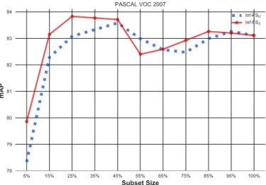
Acronym Type Class Comp. complexity LLCFS [9] f u N/A LS [28] f u N/A MCFS [29] f u N/A Relief-F [30] f s O(iT nG) MI [34] f s O(T2n2) Fisher [33] f s O(T n) ECFS [42], [43] f s O(T n+n2) ILFS [22] f s O(n2.37+in+T+G) CFS [47] f u O(n22T) UDFS [52] f u N/A DGUFS [44] w u N/A FSASL [45] w u O(n3+T n2) UFSOL [46] w u O(iT Gn3) RFE [47] w s O(T2nlog2n) FSV [11] e s O(T2n2) LASSO (hinged) [55] (unhinged) [56] e s O(T2n2) NHTP [59] e s N/A Inf-FSU f u O(n3(1 +T)) Inf-FSS f s O(T2+n3(1 +T)) TABLE 1
Feature selection approaches considered in the experiments of Sec.4. The methods follow the taxonomy of Sec.2, and are characterized by
type(f=filter, w=wrapper, e=embedded),class(u = unsupervised, s = supervised) andcomputational complexity. As for the complexity,Tis the number of samples,nis the number of initial features,iis the number of iterations in the case of iterative algorithms, andGis the
number of classes.
filter, wrapper and embedded approaches. Tab.1lists the methods
included in the experiments, reporting their type (f = filters,
w = wrappers, e = embedded methods), and their class ( s =
supervised or u = unsupervised). Additionally, the table shows
the computational complexity whereas it has been provided.
The experiments are performed on 11 different publicly
available benchmarks, whose characteristics are summarized in
Table 2. The benchmarks allow to evaluate the proposed
ap-proach on supervised classification problems, focusing first on small-sample, high-dimensional scenarios, studying the strengths and weaknesses of the unsupervised and supervised Inf-FS on heterogeneous datasets, dealing then with features produced by deep learning algorithms. All of these experiments evaluate the feature selection approaches when they are constrained to provide
a definite numberb of features; differentb’s are considered (see
in the following sections). In addition, we evaluate the automatic subset selection capability, where the optimal number of features has also to be decided. A conclusive statistics shows the Inf-FS framework as the most versatile and effective generpurpose al-gorithm among the considered competitors. All of the (MATLAB) code is available athttp://demo.polr.me/0.
4.1 Challenge 1: Small-sample, high-dimensional Treating few samples described by many features is a traditional feature selection challenge. For example, in the medical field [69] observations are often difficult to collect (e.g., in the case of rare diseases), while the number of measurements performed on each sample can easily reach the order of thousands (e.g., set of DNA sequences). The small-sample, high-dimensional scenario holds in
many other fields like business intelligence [70], geoscience [71] and the automatic analysis of behavioural cues and social sig-nals [72], [73]).
Here we consider five widely used small-sample,
high-dimensional 2-class microarray datasets: Colon [12],
Lym-phoma[13], Leukemia[13], Lung [14], andProstate[15]. They have been chosen for their variability in terms of number of
features (from 2000 to 12533, see Tab. 2) which characterize
45 to 181 samples, because they deal with balanced and unbal-anced classes, and because they are widely used in the literature. An exhaustive list of microarray small-sample, high-dimensional
datasets can be found inhttps://bit.ly/2OSlOfv, while an essay on
generic microarray datasets can be found in [74].
The experimental protocol consists in splitting the samples of the dataset in 70% for training and 30% for testing. The
training procedure consists in building the matrixAas described
in Sections3.1 and3.2. In the case of Inf-FSS, the class labels
are taken into account, while in the unsupervised case they are ignored. After the training, a selection of the ranked features
is considered, by keeping the top-b features, with b variable.
The selected features are used to train a linear SVM, where a 5-fold cross-validation on training data is used to set the best
C regularization parameter. The same experimental protocol has
been applied to all the comparative feature selection approaches.
The number b of selected features varies (i.e., b =10, 50,
100, 150, and 200) in order to show the performance at different regimes. The performance is specified in terms of classification accuracy. In order to avoid any bias induced by a particularly favourable split, this procedure is repeated 20 times by shuffling the data (keeping training and testing separated) and the results are averaged over the trials. A cross-validation is carried out on each training partition of the datasets to select the{α}parameters introduced in Sec.3.1and3.2.
Fig.1depicts the results: on theleft, the average performance obtained over all of the datasets by the unsupervised approaches
are reported; on theright, supervised approaches are shown.
On Fig. 1 (left and right), it can be seen that in both the
unsupervised and supervised case, the performance improves substantially with the number of the selected features up to a knee around 50 features; after 150 features, in general, the performance tends to saturate. On the left, it can be seen that
Inf-FSU outperforms the existing methods with a mild but consistent
average gap. On the right, Inf-FSS achieves definitely the best
performance, in particular when the number of selected features is fixed to be small (from 10 to 100).
Comparing Inf-FSU and Inf-FSS (Fig. 1, left and right) one
can see that, in general, Inf-FSSworks better than Inf-FSU, since it
uses class-label information to guide the FS process. Nonetheless, it is worth knowing (no curves are reported here) that on some datasets (COLON, LEUKEMIA and LUNG) the performance of the two approaches is comparable. This interesting aspect will be further discussed in Sec.4.4and Sec.4.3.
4.2 Challenge 2: Inf-FSU VS Inf-FSS
This section compares the supervised and unsupervised versions of Inf-FS. Essentially, the difference between the two approaches consists of the type of functions used for weighting the graph.
In fact, Inf-FSU does not employ any class-label information
according to Eq. 2, while Inf-FSS is a combination of three
10 50 100 150 200 Subset Size 65 70 75 80 85 90 95 Accuracy
MICROARRAY - PERFORMANCE (UNSUPERVISED)
CFS [48] DGUFS [51] FSASL [52] LLCFS [37] LS [35] MCFS [36] UDFS [57] UFSOL [53] Inf-FSU [8] 10 50 100 150 200 Subset Size 71 76 81 86 91 96 Accuracy
MICROARRAY - PERFORMANCE (SUPERVISED)
NHTP [59] ECFS [42] Fisher [33] FSV [11] ILFS [22] LASSOU [56] LASSOH [55] MI [34] ReliefF [30] RFE [47] Inf-FSS
Fig. 1. Classification results on the small-sample, high-dimensional challenge. On the left, the average performance curves for unsupervised approaches, and on the right, supervised methods are shown. In all of the cases, the performance is measured at different numbers of selected features (on the x-axis).
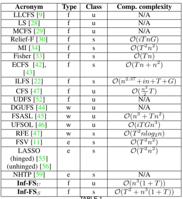
10 50 100 150 200 Subset Size 52 55 58 61 64 67 70 73 76 79 82 85 88 91 94 Accuracy Performance on GISETTE NHTP CFS DGUFS ECFS Fisher FSASL FSV ILFS LASSOU LASSOH LLCFS LS MCFS MI ReliefF RFE UDFS UFSOL Inf-FSU Inf-FSS 10 50 100 150 200 Subset Size 52 55 58 61 64 67 70 73 76 79 82 85 88 Accuracy Performance on GINA NHTP CFS DGUFS ECFS Fisher FSASL FSV ILFS LASSOU LASSOH LLCFS LS MCFS MI ReliefF RFE UDFS UFSOL Inf-FSU Inf-FSS 10 50 100 150 200 Subset Size 49 51 53 55 57 59 61 63 65 67 69 71 73 75 77 79 81 83 85 87 89 91 93 Accuracy Performance on DEXTER NHTP CFS DGUFS ECFS Fisher FSASL FSV ILFS LASSOU LASSOH LLCFS LS MCFS MI ReliefF RFE UDFS UFSOL Inf-FSU Inf-FSS 10 50 100 150 200 Subset Size 49 52 55 58 61 64 Accuracy Performance on MADELON NHTP CFS DGUFS ECFS Fisher FSASL FSV ILFS LASSOU LASSOH LLCFS LS MCFS MI ReliefF RFE UDFS UFSOL Inf-FSU Inf-FSS
Fig. 2. Comparison between Inf-FSUand Inf-FSS. All the supervised approaches are reported by solid lines and the unsupervised ones by dotted lines. Results are expressed in terms of classification accuracy (%).
Dataset Ref. #Samples #Classes #Feat. few train unbal. (+/-) overlap noise sparse COLON [12] 62 2 2K X (40/22) n.s. X LEUKEMIA [13] 72 2 7129 X (47/25) n.s. X LUNG [14] 181 2 12533 X (31/150) n.s. X LYMPHOMA [13] 45 2 4026 X (23/22) n.s. PROSTATE [15] 102 2 6033 X (50/52) n.s. DEXTER [18] 2600 2 20K (1,3K/1,3K) X X X GISETTE [17] 6000 2 5K (3K/3K) X X GINA [16] 3153 2 970 (1,5K/1,6K) X MADELON [17] 2000 2 500 (1K/1K) X X VOC 2007 [19] 10K 20 4096 X X X CalTech 101 [20] 10K 102 4096 X X X TABLE 2
Datasets and the challenges for the feature selection scenario. The abbreviationn.s.stands fornot specified(for example, in the DNA microarray datasets, no information on class overlap is given in advance).
criterion and mutual information, see Eq.6). When the difficulty
of a classification problem depends on classes that overlap,
Inf-FSS can naturally favour those features that best represent the
explanatory factors of the dissimilarity among the classes. On the
other side, Inf-FSS suffers when features are severely correlated,
even if they are representative for a specific class. In this case,
variance and correlation computed by Inf-FSUdo represent a very
convenient option.
To validate these considerations, we consider four additional
datasets from the NIPS feature selection challenge, namely:
DEXTER [18], GISETTE, MADELON [17] and GINA [16].
GISETTE and GINA present severely overlapped classes. Indeed,
the GISETTE dataset [75] has instances of “4” and “9”, two
con-fusable handwritten digits (i.e., two overlapped classes) extracted
from the MNIST data [76]. Features consist of normalized pixels
and quantities derived from their combination.
The task of GINA is again handwritten digit recognition, but
in this case, the two classes areeven and odd 2-digit numbers.
Obviously, only the unit digit is informative. In addition to the overlapping issues among the single digits (which are taken again from the MNIST data), a further consistent overlap is caused by the digits indicating the tens.
As for a dataset with non-descriptive features, we selected
the DEXTER dataset [18], composed by sparse continuous
bag-of-words histograms, extracted from the Reuters text
categoriza-tion benchmark [75]. Noise is coming from 10,053 distractors
(features having no discriminative power) put voluntarily in the dataset.
A benchmark where Inf-FSU should perform comparably if
not superior to Inf-FSS is MADELON [17]. In fact, MADELON
is an artificial dataset containing data points grouped in 32 clusters placed on the vertices of a five-dimensional hypercube and randomly labelled +1 or -1. The five dimensions constitute 5 informative features. 15 linear combinations of those features were added to form a set of 20 (redundant) informative features. Based on those 20 features one must separate the examples into the 2 classes (corresponding to the +1, -1 labels). A number of distractor features (480) called “probes” have no predictive power. Other than this, correlated features are present.
The results are shown in Fig.2. In general, Inf-FSS
outper-forms Inf-FSU on DEXTER, GINA and GISETTE and achieves
a absolute top performance in most of the cases. On the other
hand, Inf-FSUachieves a better performance on MADELON at 10
features w.r.t. the supervised counterpart, by discarding the several
correlated features in the set, and behaves comparably with Inf-FSSat the other regimes.
Considering each dataset separately, on GISETTE (Fig.2
top-left) Inf-FSSbetters all the comparative approaches when using 10
features, having NHTP close to its performance, while in the other supervised cases the gap is substantial. Unsupervised approaches do comparably to supervised ones when it comes to 10 features, but this is probably due to the fact that 10 features are definitely too few over the 5K which are originally available, and where many of them are probably equally useful. In fact, when the number of allowed features is growing (150, 200), it is visible that most supervised approaches better the unsupervised ones. Among
the unsupervised approaches, our Inf-FSU ranks approximately
third after LLCFS [9] and LS [28], since the former is driven
by variance and correlation, and this does not allow to unveil
features which are overlapped among classes. Notably, LLCFS [9]
and LS [28] select features which are locality preserving, i.e.,
which agree on a clustering over the data. We may think that this clustering is capable to naturally separating the digits data,
providing a more powerful solution than Inf-FSU.
ON GINA instead (Fig. 2 top-right), supervised approaches
show immediately at 10 features a consistent advantage over the
unsupervised methods. Here, Inf-FSS is on pair with the mutual
information MI [34] and the Fisher approach [33]. In facts,
Inf-FSS is containing both of them in the adjacency matrixA (see
Sec. 3.2), and they are useful to highlight features that do not
overlap across classes, i.e., which are non linearly correlated with
the class information. Inf-FSU gives here the worst performances,
ranking approximately fourth with respect to slower and more
complex approaches (MCFS [29], LLCFS [9], DGUFS [44])
which once again exploit the hypothesis that data is organized
in multiple clusters which we are ignoring with Inf-FSU.
DEXTER (Fig. 2 bottom-left) has the highest number of
features (20K) so that restricting to only 10-200 features opens to many equivalent selections, which anyway are better individuated
by INf-FSS (among the supervised approaches, except the 10
features case where LASSO shows to be better) and by INf-FSU
(among the unsupervised approaches, on pair with LS [28] which
is better at 100-200 features).
On MADELON we already have discussed above the results of Fig.2(bottom-right) .
5% 10% 15% 20% 25%
Subset Size
55 57 59 61 63 65 67 69 71 73 75 77 79 81 83mAP
Performance on PASCAL VOC 2007
NHTP CFS DGUFS ECFS Fisher FSV ILFS LLCFS LS MCFS MI ReliefF RFE UDFS UFSOL Inf-FSU Inf-FSS 5% 10% 15% 20% 25%
Subset Size
87 88 89 90 91 92Accuracy
Performance on CALTECH 101 NHTP CFS DGUFS ECFS Fisher FSASL FSV ILFS LLCFS LS MCFS MI ReliefF RFE UDFS UFSOL Inf-FSU Inf-FSSFig. 3. Performance achieved for the image classification task reported in terms of mAP (VOC 2007) and classification accuracy (Caltech-101) while selecting the first 5%, 10%, 15%, 20%, and 25% features. Solid lines individuate supervised feature selection approaches, dotted lines indicate unsupervised approaches. 10 50 100 150 200 Subset Size 1 2 3 4 5 6 7 8 9 Avg. Rank RANKING (UNSUPERVISED) CFS [47] DGUFS [44] FSASL [45] LLCFS [9] LS [28] MCFS [29] UDFS [52] UFSOL [46] Inf-FSU [23] 10 50 100 150 200 Subset Size 1 2 3 4 5 6 7 8 9 Avg. Rank RANKING (SUPERVISED) NHTP [59] ECFS [42] Fisher [33] FSV [11] ILFS [22] LASSOU [56] LASSOH [55] MI [34] ReliefF [30] RFE [47] Inf-FSS
Fig. 4. Bubble plot showing the average ranking performance (y-axis) overall the datasets while increasing the number of selected features for the unsupervised approaches (left) and supervised ones (right). The area of each circle is proportional to the variance of the ranking.
4.3 Challenge 3: Feature selection on CNN Features Applying feature selection on deep learning-based cues is a recent
trend in image recognition [77], [78]. In fact, recent studies
show that feature learning and deep learning are not immune to produce redundant or introduce useless information in the learned
representations. For example, [78] proposed a generic framework
for network compression and acceleration where CNNs are pruned by removing neurons with least importance, resulting in more robust networks. Neuron importance scores (usually associated to the last layer of the network, before classification) are computed
by Inf-FSUas a function of the importance of all the other neurons
in the layer.
In this subsection, we evaluate the performance of the
pro-posed approach on features learned by the very deep ConvNet [21]
framework, where the pre-trained model used for the ImageNet Large-Scale Visual Recognition Challenge 2014 (ILSVRC) is
adopted. We use the4,096-dimension activations of the last layer
as image descriptors (L2-normalized afterwards), and we focus on the CALTECH 101 and PASCAL VOC-2007 datasets. These datasets allow for a systematic testing of the feature selection approaches taken into account in this paper, in a reasonable amount of time. We omit to choose other benchmarks (Imagenet for example) since for some of the comparative methods (LASSO
and MCFS) the running time for a single trial is exceeding the week. Indeed, for each comparative approach, we perform a total
of200runs.
According to the experimental protocol provided by the VOC challenge, a one-vs-rest SVM classifier is trained for each class (where cross-validation is used to find the best parameter C) and
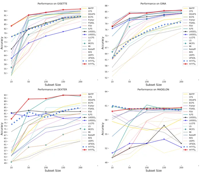
evaluated independently. Fig. 3 reports the performance curves
obtained with the 18 feature selection approaches (solid lines for supervised approaches, dotted lines for unsupervised ones). In this case, the goal was to investigate the classification while keeping the first 5%, 10%, 15%, 20%, 25% of the features, corresponding to 205, 410, 614, 819 and 1024 characteristics.
From Fig. 3 (Left), it can be seen that the supervised
Inf-F SS reaches good performance in general, with a slightly
supe-rior performance w.r.t. the eigenvector centrality-based approach (ECFS). In general, the supervised approaches are organized into two groups, the most performing ones are the INFFS, ECFS, that, together with MI and ILFS gives an increase in the classification performance when adding more features. The other supervised approaches (RFE, FSV and RELIEF) seems to have a lower trend. Viceversa, all of the unsupervised approaches are more consistent among themselves, with Inf-FS positioning in the top 3 positions after LS and LLCFS. In the case of CALTECH 101 it is easy to
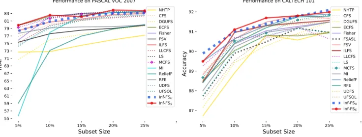
5% 15% 25% 35% 45% 55% 65% 75% 85% 95% 100% Subset Size 78 79 80 81 82 83 84 mAP PASCAL VOC 2007 Inf-FSU Inf-FSS
Fig. 5. Varying the cardinality of the selected features on VOC 2007. Mean average precision instead of classification accuracy is provided here.
see that the task is easier, with all of the approaches positioning in
a narrow band of performance. Notably, Inf-FSS and Inf-FSU are
on pair at the top position.
On the PASCAL 2007, we performed an additional experi-ment, aimed at exploring the performances when spanning the
number of features retained from 5% to 100% (Fig.5). The idea is
to check how much difference holds when keeping a small number of features with respect to the whole set. In fact, feature selection approaches often represent a compromise between admitting a lower classification performance at the price of a faster time of task
execution [25]. We apply both Inf-FSSand Inf-FSU. Noteworthy,
both of the approaches provide features subsets leading to a perfor-mance (mAP) superior to the one obtained with the entire pool. In
particular, with 25% of features, Inf-FSS raises the classification
performances of barely 1 percentage point (83.8% against 83.1% fo the full set). Better performances are obtained in the range of
25%-45%. The Inf-FSS shows that there is a 10% of features
ranked last which cause a slight bending of the performances
(see the 90%-100% range). Inf-FSU has a similar behaviour, but
lower in mAP score: The peak is at 45% of features (83.6%). To further explore the behavior of the approach in the range of
best performance (25%-45% for Inf-FSS and 35%-45% for
Inf-FSU) we perform a fine-grained cardinality analysis reaching the
absolute best of Inf-FSS at 31.5% features (84.18% mAP) and
36.5% for Inf-FSU (83.91% mAP).
4.4 The versatility of Inf-FSU and Inf-FSS
In this section we want to summarize the diverse experiments carried out so far, demonstrating that one of the most valuable
merit of the Inf-FS framework is thatit applies favorably on every
genre of feature selection scenario. To this sake, we set up in
Fig.4two bubble-plots showing the average ranking (the lower,
the better) for each compared approach (y-axis), considering all of the used datasets (except CALTECH 101 and PASCAL VOC where LASSO did not apply, and where we evaluated different numbers of features), separating the unsupervised and supervised approaches that we have considered in the experiments.
In practice, the ranking represents the position of an approach (as classification accuracy) with respect to all the others. In the case a given approach has the best accuracy for a given benchmark,
its rank on that benchmark is 1, in the case it gives the second-best accuracy the rank is 2, and so on. The average ranking shows how
an approach, independently on the accuracy score, isgenerically
betterthan the others, exhibiting a relative ordering.
The average ranking is computed with respect to different subsets of features (x-axis), and is enriched by the standard deviation in the ranking (how consistently an approach had a particular rank), depicted by the size of the blob (the larger the size, the higher the ranking variance).
The figures convey a clear message, since both Inf-FS unsu-pervised and suunsu-pervised have the best rank, with a variance of 0.23 which indicates a stable behavior of both the approaches. Notably,
Inf-FSS is definitely the most effective choice when it comes
to few features selected; the mutual information-based MI [34]
and the Fisher criterion for feature selection [33] follow. In the
case of unsupervised approaches, Inf-FSU is first, followed by the
clustering based approaches LS [28] and MCFS [29].
4.5 Challenge 4: Automatic Subset Selection
In this section, we test the process of selecting a subset of relevant features from the ranking provided by Inf-FS, explained in Sec.3.6.
To this sake, we repeat all of the experiments with Inf-FSSand
Inf-FSU on the 11 datasets examined so far, selecting as relevant
features the ones indicated by the cluster which includes the first-ranked feature, and using them for the classification tasks. As comparative approach, we consider LASSO learned with hinge loss [55] and unhinged loss [56], since it is the only which allows to automatically select a precise number of features, that is, the ones which survive the shrinking process during the training stage. In particular, we individuate the best-performing LASSO by 5-fold cross-validating the regularization parameter over the training set of each benchmark, for both the hinged and unhinged versions.
The results are reported in Table3
For each pair< dataset, method >, we report four different
quantities: in the Subset column we show in round brackets
the number of selected features, and alongside the classification
accuracy obtained with that number of features. In theBest Prev.
Perf.column, we report in round brackets the number of features
that provided the best performance obtainedin the previous
experi-ments(following on the right). In the table, bold scores indicate the highest classification performance among the scores obtained by the automatic selection of feature subset, not the highest absolute.
From the results, several observations can be drawn:
• The automatic selection of the number of features allow
Inf-FSU and Inf-FSS to provide higher performances than
LASSO on 9 out of 11 cases, with LASSO unhinged beating the Inf-FS framework on GISETTE and GINA;
• Tightly connected with the previous point, and worth noting,
the Inf-FS framework selects definitely less features than the LASSO approaches (apart from the microarray datasets, where anyway LASSO unhinged is giving scarce perfor-mance). LASSO unhinged tends to keep features in a number which is highly variable; for example, it suggests a very large amount of features (2126 for GISETTE) or very few (the five microarray datasets); this seems to be correlated with the number of samples in the dataset, that, for the microarray datasets, is quite small. LASSO hinge appears to be more stable (but it gives the highest number of features).
• Inf-FSSrequires for all of the datasets less features than