Deep Learning Algorithms for Cardiac Image Classification and Landmark Detection

Lunds tekniska högskola

Deep Learning Algorithms for Cardiac

Image Classification and Landmark Detection

Anton

HOLM

Supervisors:

Einar

_HEIBERG

Niels Christian

_OVERGAARD

Abstract

With the increase in computational power, deep learning algorithms have become an active field of re-search over the last 7 years. These data-driven machine learning algorithms have produced good results in many applications, image analysis being one of them. Today, many image analysis tasks in the medical field are done manually, taking valuable time and effort from professionals. Automating some of these tasks could relieve work-load and speed up the healthcare process.

In this thesis, the potential use of deep learning algorithms for medical image analysis will be evaluated. Two problems will be investigated, cardiac image classification and landmark detection in cardiac images. The algorithms used will be based on two existing deep learning algorithms, the U-net and AlexNet. The deep learning algorithms will be implemented in the deep learning software Caffe, and all training and testing will be ran on an Amazon Web Services instance. The data used for training, testing and validation are provided by the Department of Clinical Physiology at Lund University Hospital. This data is augmented by scaling and rotation to provide a larger and more representative data set for training. The trained algorithm for image classification achieved 98.8% accuracy on validation data, while the algorithm for landmark detection achieved approximately 95 % accuracy on validation data.

The image classification algorithms worked well, and it serves as a proof of concept with the potential of being able to solved more clinically difficult problems. With the high accuracy of the landmark detection algorithm largely being due to an imbalance in class distribution, this algorithm, while showing some promise, needs more work to be clinically useful.

Contents

1 Introduction 3

2 Aim 5

3 Theory 6

3.1 Neural networks . . . 6

3.2 Convolutional neural networks . . . 6

3.3 AlexNet . . . 7 3.4 U-net . . . 7 3.5 Loss function . . . 8 3.6 Hyper-parameters . . . 9 3.7 Data augmentation . . . 9 4 Method 11 4.1 Networks . . . 11 4.2 Training environment . . . 11 4.2.1 Microsoft Azure . . . 11 4.2.2 Caffe . . . 11 4.2.3 MatLab . . . 11 4.2.4 Hardware . . . 11 4.3 Data . . . 11 4.3.1 Landmark Detection . . . 12 4.3.2 View-plane Classification . . . 12 4.4 Data augmentation . . . 13 4.5 Training . . . 13 5 Results 14 5.1 Landmark detection . . . 14 5.2 Image Classification . . . 14 6 Discussion 17 6.1 Learning environment . . . 17 6.1.1 Implementation . . . 17 6.2 Landmark Detection . . . 17 6.3 Image Classification . . . 18 6.4 Future work . . . 19 7 Conclusions 20 8 Appendix 22 8.1 Appendix 1 . . . 22

1

Introduction

Many applications in cardiac image analysis, such as segmenting the ventricles or finding anatomical landmarks are time-consuming. There are automatic algorithms that perform some of these tasks, how-ever some tasks are still carried out entirely manually and algorithms at hand often need supervision as they are not as accurate as a human. This means that, in addition to occupying professionals with a rather basic task, the results are dependent on the individual who performs the task. It would thus be desirable to have algorithms which can perform image analysis automatically, with results comparable to those of a medical professional, saving both time and assuring consistent results.

In recent years there has been a surge of machine learning algorithms in image analysis and computer vision research. One branch of machine learning which has attracted a lot of attention and shown to be successful in many fields, especially image analysis and processing, is deep learning. These algorithms are based on Artificial Neural Networks, which has been an active field of research since the 1960’s [4]. However, limitations in computational power prevented them from developing much further.

The increase in computational power and the use of cloud services have in the last decade provided the opportunity to take these algorithms to the next level. A simple Neural Network consists of a few layers and less than a hundred neurons. The new networks that have been developed in recent years are much larger. SuperVision is a network that is made to classify images from the ImageNet database. It contains 7 layers, roughly 650 000 neurons and 630 million parameters, to train such a network takes several days even on multiple computers [7]. Networks which contains a large number of layers, neurons and parameters, such as SuperVison, have been given the name deep neural networks, or deep learning algorithms.

The position and the orientation from which the image is taken will determine which anatomical struc-tures can be seen in the image. The image could in theory be taken from any direction, however the most common is that it is taken in one of the three main planes of the body, the Coronal, Sagittal, or Axial plane. These planes are illustrated in Figure 2.

Figure 2: Planes of the body [3]

The direction and depth in which the image is taken defines the so-called ’view’ of the image. Images of the same view usually look similar, and differs significantly from other views.

The first task which is explored in this thesis is landmark detection in cardiac images. Depending on the view the image is taken in, there are different anatomical landmarks which could be detected. These landmarks can then be used by several other algorithms, for example for tracking the movement of the Atrio-Ventricular (AV) plane, to provide information about heart diseases [1].

The second task which is part of this thesis is identifying in which view the cardiac image is taken. Specifically, the views in which landmark detection can be applied is of interest. The three views which are of interest for landmark detection in this thesis are the 2-chamber, 3-chamber, and 4-chamber views. Examples of these can be found in Figure 9. In the 2-chamber view you see the Left Ventricle and the Left Atrium, in the 3-chamber view you also see the Aorta and, further, in the 4-chamber view you see in the Left- and Right Atrium as well as the Left- and Right Ventricle

There are algorithms available today that can accurately identify the view of the image. However, if it can be shown that a deep learning algorithm can solve this task well, or even better than existing algorithms it could be further developed to perform also tasks for which there today are no automatic algorithms available, for example analyzing images of an enlarged hearts.

Many of the current automatic methods that do image segmentation, landmark detection or other tasks, not based on machine Learning algorithms, are very application dependent. This means that even just a slight change in the description of the problem, e.g. you want to detect slightly different landmarks, renders the algorithm useless and much time and effort must be spent adjusting it to the new task at hand. Using machine learning, the network could easily be retrained on new data.

Deep learning algorithms for segmentation have been published in the last five years [7] and have shown good results. Not nearly as much efforts, however, have gone into landmark detection and this is still a task where deep learning algorithms need to be evaluated.

The deep learning algorithms which are used for segmentation, and will be used as a starting point for the landmark detection algorithms, are so calledsupervised learning algorithms. This means that they use data which come with a ’ground truth’, which in the case of segmentation is e.g. a mask showing where in the image the segments are, or for landmark detection, integer values identifying the different pixels where the landmarks are located. In other words, they use data that has been analyzed by a human who has provided the expected output given the input image.

The algorithms use these data to ’learn’ how to perform the task. In general, the more data the algorithm have available to learn from, the better it will be at performing the task [8]. In hospitals around the world there are many cardiac images in which the landmarks have been manually identified. Thus, there is an opportunity to gather large amounts of data that a deep learning algorithm can use. With the possibility of gathering large amounts of data, and based on the good results deep learning algorithms have provided in other Bio-medical imaging tasks, Thus, there is a potential for deep learning algorithms to achieve good results in landmark detection as well.

As mentioned above, most traditional image analysis methods are application dependent. For machine learning algorithms this may not be true. Even if a specific machine learning algorithm specializes in performing one task, it has been shown that using existing machine learning algorithms on new tasks, with only some slight modifications of the parameters, results not only in an algorithm that performs equally well as creating a new one from scratch, but can actually increase the performance, and enable the network to be trained with less data [10] et al. This is a technique called Transfer Learning. This principle will be used in this thesis where an established deep learning algorithm performing segmenta-tion of the left ventricle will be used as a starting point.

2

Aim

The aim of this thesis was to evaluate the potential use of deep learning algorithms in landmark detection and view-plane classification in cardiac images, using existing deep learning algorithms, specifically the U-net [11], and AlexNet. In more detail, this thesis includes evaluating different parameter setting and data augmentation for training the networks in an attempt to achieve algorithms which could be used clinically. Furthermore, exploring some of the available software platforms for developing deep learning algorithms, assessing their uses and downsides was also in scope.

3

Theory

3.1

Neural networks

Neural Networks are a set of machine-learning algorithms, modeled loosely after the human brain. They use a cascade of multiple layers of nonlinear processing units for feature extraction and transformation. Each of these layers uses the output from the previous layer as input. They learn in a supervised and/or unsupervised manner, using gradient descent defined on a loss function which gives a measure on how well the algorithm performs the task at hand based on the output of the algorithm and the ground truth on the given training example via back-propagation. Neural Network algorithms were first suggested in the 1950s and 60s, with training via back-propagation developed in the 1970s, but it wasn’t until the late 80s it was popularized in the machine learning community [2].

3.2

Convolutional neural networks

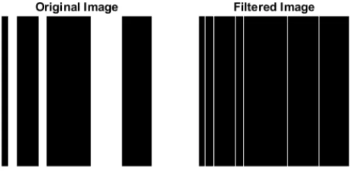
A Convolutional Neural Network (CNN) is a Neural Network which uses convolution, also known as filtering of the input, which in the case of CNNs is an image, in the feature extraction step of the algorithm. In this process, a kernel, also known as a filter, slides over the image performing a convolution at each location. The result is a new image which contains the characteristics of the image defined by the kernel at all location in the original image. In Figure 3 the result of using a kernel which extracts edges in vertical direction, i.e. rapid changes in brightness, on an image can be seen.

Figure 3: Edge-detection filter applied on image

One example of a vertical edge detecting kernel is 1 −1. When training a CNN, one of the things which changes is the values inside the kernel of each convolution layer. The size of the kernel is predefined by the user and can be different for each convolution layer.

After a convolution has been performed an activation function is applied to the output. Multiple convo-lutions followed by an activation layer can be added after each other. There are many types of activation functions which may be used, including sigmoids, step-functions or linear rectifying units. The task of these activation functions is to add non-linearity to the network. Without these functions the entire net-work would be a series of linear operations, which could be replaced by a single linear operation, i.e. one layer. As most tasks in real-life are non-linear, a linear algorithm would not be able to solve these tasks in a satisfactory manner. Hence non-linearity is needed to be able to solve a much wider range of problems. The next step in a CNN is a pooling layer. The most commonly used is the so-called max-pooling operation. Typically, for each 2-by-2 square in the image the largest value is selected and replaces the square, reducing the size of the image by a factor 2. A visualization of this operation can be seen in Figure 4. These operations are then cascaded in layers until the satisfactory level of detail extraction has been achieved.

Figure 4: Max-pooling operation [6]

Following these operation is a fully-connected neural network. This is a traditional neural network which connects each output in the following layer to all the input of the previous layer. The idea is that once the local features in the image have been extracted in the first part, the fully-connected network is trained to recognize which features are present and how they are orientated, both spatially in the image and in relations to each other, for each type of image it is being trained to recognize. This fully connected layer is in practice a series of weighted inner products. The weights of all these inner product operations is what changes during training of a CNN. An example of how a CNN could look is shown in Figure 5.

Figure 5: Example of a Convolutional neural network [9]

3.3

AlexNet

AlexNet is a Convolutional Neural Network consisting of 8 layers. The first 5 layers are convolutional, followed by 3 fully connected layers. This makes it quite a small network compared to others with similar performance. When competing in the ImageNet Large Scale Visual Recognition Challenge, which it won in 2012, it had to classify an image as one of 1000 different classes. Which it was able to do with a top-5 error of 15.3%.

3.4

U-net

The U-net architecture is a type of CNN with modifications making it appropriate for segmenting areas in an image. The first part of the network, which extracts the local features of the image is the same as in a standard CNN. The fully-connected network which follows is replaced by layers consisting of convolutions, activation-functions and up-convolution operations. The structure of a U-net is depicted in Figure 7. Where a standard CNN gives a single integer as output for an image, also called a label, a U-net architecture gives a label to each individual pixel in the image. An output like this where each pixel is assigned a label is ideal for segmentation. The simplest example would be if a label of 0 correspond to background and a label of 1 correspond to the area which is being segmented. An example of an image and its labelled segmentation mask is shown in Figure 6.

Figure 6: Segmentation of an image [5]

Figure 7: U-net Structure [11]

3.5

Loss function

The loss function is the driving force of the learning of the network. It gives a measurement of how well the algorithm is performing the task which it tries to solve. In each iteration of training the network, the parameters of the network are changed based on the gradient of the loss function, using gradient decent optimization.

A loss function should produce a large value when the output of the network does not match the ground-truth of the input and a small value when the output of the network matches the ground-ground-truth well.

With this rather vague requirement, one could think of many different functions which could be a loss function. One of the simplest being the Euclidean Loss Function, which takes the Euclidean distance between the output and the ground-truth. This is a loss function which is being used on some deep learning algorithms, but it is limited to only be applicable on algorithms which produces a single value as an output. Therefore, it couldn’t be used on a U-Net algorithm, which produces a matrix as output. One of the more common loss functions to be used for Convolutional Neural Network algorithms is the Soft-Max loss function. This is a generalization of the binary Logistic Regression classifier for multiple classes. The typical implementation of the loss function does not differentiate between classes, meaning that miss-classifying a pixel as class 1, when it should be class 0 produces the same amount of loss as miss-classifying a pixel as class 0, when it should be class 1.

A variation of the Soft-Max loss function is the weighted Soft-Max loss function, where the different classes are given a weight, changing how much a miss-classification of that class contributes to the loss function. A weighted loss function is typically used when there is a discrepancy in the amount of data between classes.

3.6

Hyper-parameters

For convolutional neural networks there are three hyper parameters which can be changed to vary the behaviour of the network during training.

Firstly, the initial learning rate, which controls how much the parameters in the network are changed in each training iteration. This learning rate can be kept constant throughout the whole training process or decrease over time as the network gets closer to an optimal solution.

One technique to prevent the algorithm getting stuck in a local minimum is to use a Momentum term. This term adds a fraction of the previous parameter update to the current one.

∆ωij(t) =µi∇f(yi) +m∆ωij(t−1)

In the equation above, the parameter update for the current iteration,∆ωij(t), is described by the

learn-ing rateµi, the gradient for the current iteration∇f(yi)and finally the momentum termm∆ωij(t−1)

which is the parameter update from the previous iteration scaled by the parameterm. The parameter

mis called the momentum hyper-parameter.

To reduce over-fitting of the network, a regularization is added to the training criterion. This regulariza-tion encourages the parameters of the network to be close to zero by penalizing values that gets to large. A so-called weight decay hyper-parameter controls how strong the regularization of the network should be. In addition to these three hyper-parameters there are a number of other parameters which needs to be set before initializing training, such as batch size, maximum number of iteration and test intervals. However, these do not affect the performance of training the network.

3.7

Data augmentation

Ideally, when training a deep learning algorithm of any sort, large amounts of data is beneficial. However, especially in medical imaging, this is not always available. Even if there are many medical images in databases at hospitals around the world, only a small amount is annotated with ground-truth for the specific task and integrity regulation prevents the data to be shared freely among research groups. This creates the need for well-designed data augmentation. Data augmentation takes an existing image, along with its ground-truth and performs some modifications to the data, such as rotations, scaling, ensuring that the ground-truth is augmented the same way to create more data to be used for training from the existing data. The challenge is deciding which kind of augmentation is relevant. Performing rotation augmentations on images where this type of augmentation is not present in the real data would be of no use and could actually make the algorithm perform worse rather than better. One needs experience

of the task at hand to be able to decide what kind of augmentation could be found in the real data and only perform augmentation which are of relevance. When done correctly, data augmentation is one of the most valuable tools when at attempting to increase the performance of a deep learning algorithm.

4

Method

4.1

Networks

The deep learning algorithm that will be used as a starting point for Landmark Detection in this thesis is a variation of the U-net [11]. This algorithm was developed as an entry in the ISBI challenge for seg-mentation of neuronal structures in electron microscope stacks. The deep neural network they developed won the challenge in 2015 by a large margin.

The View-plane classification algorithm will be based on the AlexNet algorithm. This network was developed as an entry to the ImageNet Large Scale Visual Recognition Challenge in 2012, which it won. It was developed by the SuperVision group, consisting of Alex Krizhevsky, Geoffrey Hinton, and Ilya Sutskever.

4.2

Training environment

4.2.1 Microsoft Azure

Originally, the intent was to use Microsoft Azures ML studio to create the networks and run training. However, it was quickly realized that this platform did not provide the tools for pixel-wise classification, i.e. segmentation, which was needed for the landmark detection task. It was therefore abandoned and another platform which did provide the necessary tools was identified.

4.2.2 Caffe

Instead of the intended Microsoft Azure software, all training of the networks was done using the Caffe platform for deep learning. This software was developed by Berkeley Artificial Intelligence Research and is open-source to use. This is a Linux based platform, which with the complementary software for GPU computations, CUDA, utilizes the GPU instead of the CPU for computations. It provides tools for defining networks, loading data with its corresponding ground-truths, training and testing the networks and exporting the ready trained networks into different software. The networks which were used in this thesis, the U-net and AlexNet, have previously been implemented in Caffe to be used for training on datasets provided by a user.

4.2.3 MatLab

In the 2017 version of MatLab, a toolbox for Deep learning was released. Much like Caffe, it provides tools for creating networks, training, testing and validating these networks on data provided by a user. Matlab was not used in this thesis for training the networks, however, it was used for validation as trained networks from Caffe can be imported into Matlab. Augmentation of the training and testing data was also done in Matlab.

4.2.4 Hardware

All training and testing of the algorithms was done on an Amazon Web Service (AWS) for cloud compu-tations instance. The instance has a Tesla K80 GPU where all compucompu-tations during training are carried out. The resources available on the AWS were limited, meaning that the length of the training sessions had to be limited to roughly 60 hours.

4.3

Data

The data used in the thesis was collected by the Department of Clinical Physiology at Lund University Hospital. The data used for landmark detection was manually annotated to provide ground-truth. The data for view-plane classification comes with ground-truth produced by an existing algorithm, based on usage of orientation in 3D extracted from the DICOM files. The previous algorithm does currently not use any image information, but bases its classification solely on the orientation data. The results of this algorithm have been manually verified.

4.3.1 Landmark Detection

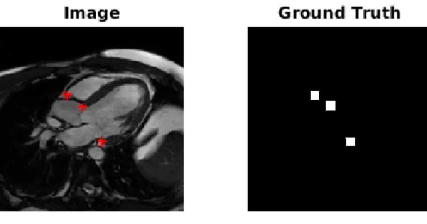
The manually annotated points for Landmark detection are given as just a pixel value for each landmark. Since the algorithm (U-net) that were used are made for segmentation, the ground-truth needed to be modified in order for it to be viewed as a segmentation problem. This was done by creating a small box of 11x11 pixels around each landmark and labelling all pixels within this box as 1, and the remaining pixels as 0. An example of this is shown in Figure 8. All images for Landmark Detection were re-sized to 200x200 pixels.

Figure 8: Example image and its ground truth for Landmark Detection. The landmarks are highlighted in the original image.

Only images in the 3-chamber view will be used for training and testing of the network.

4.3.2 View-plane Classification

For the View-plane classification data, the ground truth is a label of 2-, 3-, or 4-chamber view. Examples of how the three different views look are shown in Figure 9.

Figure 9: Examples of the different view-planes

These labels needed to be mapped to a single integer to be compatible with the algorithm. This was achieved by giving all 2-chamber images a label of 1, 3-chamber images a label of 2, and 4-chamber images a label of 3. Keeping the label of 0 as a label for any images which are none of those views. All images for View-plane classification were re-sized to 256x256 pixels.

For landmark detection there were around 300 annotated images to be used. 70% of the data was used for training the network and the remaining 30% for testing. In addition to these annotated images, there were un-annotated image which were used for validation. For view-plane classification there were around 2700 classified images available. For this task, 80% of the data was used for training, and 20% used for testing. Around 900 additional images were used for validation.

4.4

Data augmentation

In both the case of Landmark detection and View-plane classification, the data was augmented by scaling, as this is the most common augmentation which is expected to be found in real data. The data was scaled by a factor of 1.25, and 0.75, tripling the initial amount of data. The data used for Landmark Detection was also augmented by rotations, specifically 90, 180, and 270 degree rotations. A separate training run using the data with this augmentations was done to compare results.

4.5

Training

Training was carried out for roughly 500 000 iterations for the landmark detection network, and roughly 350 000 iterations for the view-plane classifications network, which resulted in approximately 50 hours of computation time in total, where the majority was spent on training the network for landmark detection. The hyper-parameters were varied for different shorter training sessions and the values which gave the best results were chosen for the longer training session. The training loss and the test accuracy were saved during training to be viewed once the training had finished.

5

Results

5.1

Landmark detection

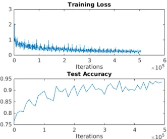
The training loss and test accuracy during training of the network for Landmark Detection, using the data augmented by rotations can be seen in Figure 10. The hyper-parameters used are stated in the caption.

Figure 10: Training-Loss and Test-Accuracy for Landmark Detection with data augmented by rotations. Initial learning rate: 5e-05, momentum: 0.99, weight decay: 5e-05.

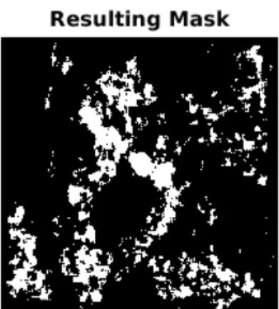
An example of a validation image, and its resulting mask, using the trained network, can be found in Figure 11. The validation data used had no existing ground truth. The training loss and test accuracy plot during training, and an example validation image, and its resulting mask, using the data augmented by scaling can be found in Appendix 1.

(a) Landmark detection validation image (b) Landmark detection validation mask

Figure 11: Example of results on validation data for landmark detection

5.2

Image Classification

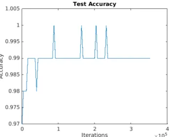
Figure 12: Test-Accuracy for View-Plane classification. Initial learning rate: 1e-04, momentum: 0.95, weight decay: 5e-04.

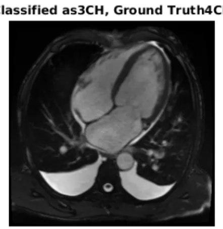
Validation of the trained network was done on a dataset of 900 images, where the network achieved an accuracy of 98.8%. Examples of validation images which were classified correctly, incorrectly and where the ground truth was incorrect are shown in Figure 13.

Out of all the miss-classified images in the validation dataset, roughly 40% were due to error in the ground-truth, while the remaining 60% were actual incorrect classifications. With this in mind, the ac-tual validation accuracy of the trained network exceeded 99%.

No images of the validation dataset were classified as the label 0, which was reserved for images which did not fit into any of the three different views. This design was chosen so the algorithm could be more general and used on datasets where images with such a label is present. However, in the dataset used for training in this thesis, all images belonged to one of the three views the algorithm is trying to differentiate between and thus no training data with label 0 existed, resulting in the algorithm not classifying any images as class 0.

(a) Example of correct classification of a validation image

(b) Example of incorrect classification of a validation image

(c) Validation image where the ground truth is incorrect, while the network classified the image correctly

6

Discussion

6.1

Learning environment

In 2017 Microsoft released a new software on their Azure platform, which supposedly supports pixel-wise classification of images. This could have been an option to use instead of Caffe.

Similarly, Matlab also released deep learning software in 2017. Both of these platforms are somewhat easier to use than the Linux-based Caffe platform, which requires quite some tinkering with prerequisites for it to work at all. Both Microsofts Azure and Matlab are ready to be used straight away without any other installations required. Matlab has also the advantage of being very easy to debug in, something that is more difficult in Caffe unless you are very familiar with Linux and its debugging system. Looking back, the best choice of software would probably have been Matlab. The reason it wasn’t chosen was because since it was very new, very little documentation for third party users exists. Matlab does provide documentation about the software and its functions, but examples of how others have done is very valuable when going into a new project. Furthermore, the networks which the algorithms used in this thesis are based on, AlexNet and U-Net, was already implemented in Caffe, without any need to convert it into a form which Matlab could have used.

6.1.1 Implementation

Provided any learning environment, fully installed with all complementary software, pre-defined networks and datasets, training a network and getting a useful result is quite simple. Setting the hyper-parameters and training parameters with desired values and running training and testing are done with only a few commands.

However, with that said, getting to this point proved to be more difficult than expected. Firstly, installing a Linux operating system, Ubuntu in this case, took time in order for it to be compatible with Caffe and the pre-defined networks it had to be a specific version of Ubuntu. Before setting up an Amazon Cloud Service, some testing on a local machine was needed. This local machine did only have a Windows operating system installed and had additional software which made the task of installing a separate operating system difficult.

The most time-consuming part of getting to the point where a network could be trained was to install all the required complimentary software for GPU computations. CUDA specifically, took time not only to install, but making sure all libraries and links were correct ensuring all the different software commu-nicated as they should. All in all, it took roughly 4 weeks before the software was installed correctly and training could be started.

The Amazon Cloud Service came with all the software already installed, however, even here some tin-kering was needed for it to work with the pre-defined networks which were to be used.

When planning for this thesis, the thought was that the majority of the time would be spent testing different configurations of the networks, different hyper-parameters and different data-augmentations. In reality, a third of the time was used to just set up the learning environment, leaving less time to modify the algorithms. Especially, more time for evaluating other data-augmentations would have been desirable.

6.2

Landmark Detection

One of the main reasons as to why the landmark detection algorithm didn’t perform well enough to be useful is that the problem was attempted to be solved as a segmentation problem, when in fact it is not a segmentation problem. The reason this approach was chosen is that segmentation is by far the most represented problem which has been solved by deep learning algorithms in medical imaging. Many example networks which perform segmentation in medical images are available to use in various software platforms, Caffe being one of them. When researching available networks, no network developed to find specific points in an image, e.g. landmarks in cardiac images was found. Therefore, the options were

either to use a segmentation network, and remodel the problem to a segmentation problem, or develop a new network more or less from scratch which is able to locate specific points in an input image. With very limited previous experience with deep learning algorithms, designing a new network seemed like a very challenging task, whilst remodeling the problem to fit a segmentation approach seemed more realistic within the given time frame of this thesis.

When presenting the landmark detection task as a segmentation problem, one of the main issues encoun-tered was the unbalance in the number of pixels from each class. As stated before, in a three-chamber cardiac image, there are three landmarks of interest. Around each of these landmarks a 11x11 box was made, and all pixels within the box was labelled as 1. In an image there is thus11·11·3 = 363 pixels with the label 1, and the remaining200·200−363 = 39647pixels have label 0, meaning that less than

1%of the pixels belong to class 1. Without a weighted loss function, the network would have classified everything as 0, and just stopped there as the few miss-classified labels 1 would not have been enough to drive any training forward. But even with a weighted loss function which prevents this, having a more balanced number of pixels for each class would likely have produced better results.

While this rather naive formulation of the problem did not produce any useful results, there are some ideas on how to improve the algorithm to possibly perform better without changing the approach to the problem.

One difficulty the network faced when trying to locate the areas around each landmark was that it was trying to find three, rather different looking areas at the same time. In the process of trying to learn how each of these areas look like, and classifying these areas correctly, many other areas in the image which are not close to any landmark were miss-classified.

If the network had to learn to find only one landmark, which has distinguished features around it which should be very similar in the different training images, it could potentially perform this task much better since it can specialize in the local structure around that specific landmark instead of trying to learn three different structures at the same time. The downside of this idea is that three separate networks would be needed for a 3-chamber view landmark detection algorithm, increasing the training time and computation time threefold.

6.3

Image Classification

While the results of the view-plane classification algorithm were good, it is still not very useful in prac-tice for cardiac MR images. This information is almost always gathered when the images are taken. If this information should however be missing, an algorithm which uses information gathered during the acquisition of the image to determine the view already exists.

There are other medical images where it could be more useful though. In ultrasound examinations, for example, image orientation is typically not available and the image classification could be very useful. Some of the few validation images where the view-plane algorithm miss-classified the view had features which rarely are found in these types of images. For example, in Figure??there are a lot of fluid present in the pleural cavity. Since very few images with the characteristic are present in the dataset, the algo-rithm is not able to determine the class correctly. With more training data, it is likely that this condition would be better represented, and thus enabling the algorithm to correctly classify also images like this. The results serve more as a proof of concept, that deep learning algorithms can perform well on finding differences in Medical images. Algorithms like this could in the very near future be trained to differentiate for example between images of an enlarged heart and a healthy heart. Further, the application doesn’t have to be limited to cardiac imaging, finding images with tumours for different organs is something which also could be an opportunity for these kind of algorithms.

In the end though, leaving the entire responsibility to classify an image as healthy or not to an algorithm is not wise. Algorithms like this will more likely serve as a decision support, perhaps going through large amounts of data and picking out images which show any kind of deviation for a medical professional to examine. This could speed up the clinical process and relieve the imaging experts from some of the more tedious work-load.

6.4

Future work

It is obvious that some more work is required to achieve an algorithm which handles the landmark detec-tion task in a satisfactory manner. If the current method of treating the problem as a segmentadetec-tion task is to be kept, the issue of having a very uneven distribution of the different classes needs to be addressed. One idea of how to do this is, prior to sending the image to the deep learning algorithm, segment out a smaller piece of the image, in which the landmark of interest lies. Also, this task could potentially be solved by a deep learning algorithm. A deep learning algorithm could be taught to identify in which re-gion of the image a particular landmark is located, and then send this smaller image into a deep learning algorithm of the type described in this thesis. With a smaller image, provided that the region around the landmark which is classified as class 1 is kept the same size, would make the distribution of classes more equal.

Another option would be to approach the problem differently, i.e. not using a network made for seg-mentation to solve the task. Using a network similar to AlexNet used for the image classification task, one could train a network to output a single integer value, representing a pixel in the image where the landmark is located. A network which outputs three integer values (or however many landmarks is being identified), representing all the landmarks in the image could also be an option. The potential problem with this, is that since no images are the same, the landmarks will always be located slightly different in different images. With a limited amount of training data, it is then difficult to represent all the different locations in which the landmark could be located. Given an image of size 200x200 pixels, the network would have to classify the image as one of 40000 classes, one class for each pixel in the image. Even for a complex network, this seems like a daunting task with much room for error. Without having tested this approach though, one can only speculate how well such a network would be at solving the task of finding landmarks in cardiac images.

7

Conclusions

From the results presented in this thesis, the conclusion is that, for view-plane classification, the deep learning algorithm worked well. The accuracy for validation data was 98.8%, where some of the miss-classified images where due to errors in the ground truth. Deep learning algorithms show some promise also for landmark detection in the sense that the output from the trained network on the validation data did classify the areas around the landmark correctly. However, in the current setting, it also classified parts of the image where no landmark is present as having a landmark, implying that modifications of the algorithm will be required to make it useful in practice.

References

[1] Seemann F, Pahlm U, Steding-Ehrenborg K, Ostenfeld E, Erlinge D, Dubois-Rande JL, Jensen SE, Atar D, Arheden H, Carlsson M, et al. Time-resolved tracking of the atrioventricular plane displace-ment in cardiovascular magnetic resonance (CMR) images. BMC Med Imaging. 2017;17(1):19. [2] Beyond Regression: New Tools for Prediction and Analysis in the Behavioral Sciences, Werbos, P.J.

https://books.google.se/books?id=z81XmgEACAAJ 1975 Harvard University

[3] Anatomical Terminology, Planes of the Body https://training.seer.cancer.gov/anatomy/body/terminology.html, Januray 2018

[4] A. G. Ivakhnenko, Valentin Grigor’evich Lapa, Cybernetics and forecasting techniques, American Elsevier Pub. Co., 1967.

[5] Siftflow Dataset, University of North Carolina, Computer Sience. http://www.cs.unc.edu/ jtighe/-Papers/ECCV10/siftflow/baseFinal.html, January 2018

[6] Convolutional Neural Networks (CNN/ConvNets) http://cs231n.github.io/convolutional-networks, January 2018

[7] Alex Krizhevsky and Sutskever, Ilya and Hinton, Geoffrey E, ImageNet Classification with Deep Convolutional Neural Networks, NIPS’12 Proceedings of the 25th International Conference on Neural Information Processing Systems - Volume 1 Pages 1097-1105 2012.

[8] Xue-wen chen, Xiaotong lin, "Big data deep learning: challenges and perspectives", IEEE Access, vol. 2, pp. 514-525, 2014.

[9] Convolutional Neural Networks (LeNet) http://deeplearning.net/tutorial/lenet.html, January 2018 [10] Wenyuan Dai, Qiang Yang, Gui-Rong Xue, and Yong Yu. 2007. Boosting for transfer learning. In Proceedings of the 24th international conference on Machine learning (ICML ’07), Zoubin Ghahra-mani (Ed.). ACM, New York, NY, USA, 193-200.

[11] Olaf Ronneberger, Philipp Fischer, Thomas Brox U-Net: Convolutional Networks for Biomedical Image Segmentation, Medical Image Computing and Computer-Assisted Intervention (MICCAI), Springer, LNCS, Vol.9351: 234–241, 2015.

[12] Geert Litjens, Thijs Kooi, Babak Ehteshami Bejnordi, Arnaud Arindra Adiyoso Setio, Francesco Ciompi, Mohsen Ghafoorian, Jeroen A.W.M. van der Laak, Bram van Ginneken, Clara I. Sánchez, A survey on deep learning in medical image analysis, Medical Image Analysis, Volume 42, 2017, Pages 60-88,.

8

Appendix

8.1

Appendix 1

Figure 14: Training Loss and Test Accuracy plots for Landmark Detection using data augmented by scaling

Figure 16: Resulting mask of example validation image using a network trained with data augmented by scaling