Fuzzy scheduling of job orders in a two-stage flowshop with batch-processing machines

(1)

Fuzzy scheduling of job orders in a two-stage ﬂowshop

with batch-processing machines

Alebachew D. Yimer, Kudret Demirli

*

Fuzzy Systems Research Laboratory, Department of Mechanical and Industrial Engineering, Concordia University, 1515 St-Catherine W., Montreal, QC, Canada H3G 1M8

Received 10 April 2007; received in revised form 1 August 2007; accepted 25 August 2007 Available online 20 September 2007

Abstract

In this paper, we present a mixed-integer fuzzy programming model and a genetic algorithm (GA) based solution approach to a scheduling problem of customer orders in a mass customizing furniture industry. Independent job orders are grouped into multiple classes based on similarity in style so that the required number of setups is minimized. The family of jobs can be partitioned into batches, where each batch consists of a set of consecutively processed jobs from the same class. If a batch is assigned to one of available parallel machines, a setup is required at the beginning of the first job in that batch. A schedule defines the way how the batches are created from the independent jobs and specifies the processing order of the batches and that of the jobs within the batches. A machine can only process one job at a time, and cannot perform any processing while undergoing a setup. The proposed formulation minimizes the total weighted flowtime while fulfilling due date requirements. The imprecision associated with estimation of setup and processing times are represented by fuzzy sets.

Keywords: Fuzzy scheduling; Batch production; Built-to-order

1. Introduction

The build-to-order (BTO) manufacturing system is a demand satisfying strategy in supply chains that are involved in assembling of customized products. It combines the characteristics of both make-to-stock (forecast driven) and make-to-order (demand driven) strategies. In a BTO system, standard component parts and non-customizable subassemblies are acquired or build in-house based on short-term forecasts, while schedules for the few customizable parts and the ﬁnal assembly are executed after detailed product speciﬁcations have been derived from booked customer orders. A BTO strategy is used to achieve economies-of-scope and improve customer service by allowing mass customization of products.

* _{Corresponding author. Tel.: +1 514 848 2424x3160; fax: +1 514 848 3175.}

E-mail addresses:[email protected](A.D. Yimer),[email protected](K. Demirli).

Available online at www.sciencedirect.com

International Journal of Approximate Reasoning 50 (2009) 117–137

(2)

Many furniture-manufacturing firms including Elran Furniture are undergoing a paradigm shift towards a built-to-order (BTO) and lean production system. In a BTO environment, firms assess specific needs of indi-vidual customers and manufacture products as per their requirements. Production of the final product is per-formed only after actual orders are received from customers. Adopting BTO processes allows firms to effectively customize their products in order to meet the specific requirements, resulting in enhanced satisfac-tion and better relasatisfac-tionship with targeted customers. BTO processes also generate tremendous manufacturing cost savings in terms of reduced raw material inventories, reduced finished goods inventories, reduced space requirements, and increased flexibility. For example, Pella Inc., a manufacturer of windows and doors for both business and individual customers, has developed a build-to-order system[24,31].

The production setting of upholstered furniture manufacturing gives a remarkable opportunity to study the significance of batch scheduling in a build-to-order environment. The upholstering process that involves fabric cutting, sewing, stuffing and assembling operations is the critical process that impacts the efficiency of the whole production scheduling. Furniture manufacturers can implement mass customization of their products by taking different combinations of variety of styles with wide range of fabric types[32]. In order to limit the variety of options available to customers, furniture designers usually specify the fabrics that appear best with each style and publish the recommended mixes in product catalogs. A limited variety gives greater responsive-ness to the market both in production time and procurement time. Agility and leanresponsive-ness in the shop floor are two important aspects that help manufacturers able to respond relatively quickly to specific customer orders. Flexibility is required in order to accommodate the dynamic workload imbalances inherent in producing dif-ferent furniture styles. The changeover times between different styles must be very short to minimize WIP at each stage of production. The jigs and fixtures used must also be relatively simple to operate and easily exchangeable. Upholstered furniture products are bulk in size and thus consume large amounts of space; therefore, manufacturers must implement a lean production system in order to keep the products moving smoothly through the plant and to the customer[31].

In many research papers, setup time is considered to be part of the processing time. Though this assumption simplifies the analysis, it adversely affects the solution quality. Many applications such as group technology manufacturing system require an explicit treatment of setup[2,32]. Recently, an important class of scheduling with setup requirements is characterized by a flowshop group-scheduling problem. The jobs are classified into families based on operation similarities, and a single setup is required on a machine if it switches processing of jobs from one family to another, but no setup is required if the jobs are from the same family[11,33,26,30,18]. The problem of scheduling jobs with family setup times on parallel machines is also addressed in[25,14,15,29]. A mixed-integer programming approach for scheduling of batch-processing machines is proposed by[8,23].

Flowshop scheduling problems are NP-hard combinatorial problems, which usually involve extremely large solution space with too many local optima. When a sequence is altered slightly, it is diﬃcult to evaluate the improvement of the objective function with respect to the global optimal solution. The highly unstructured nature of the search space makes the problem much more diﬃcult to solve. A number of constructive heuris-tics exist that can provide good solutions to the problem in a relatively short processing of time. However, many of these algorithms operate by over simplifying the problem, which may not be acceptable from the practical aspect[5,19].

Introduced by Holland in the 1970s, genetic algorithm (GA) has proved to be a successful method for solv-ing many practical optimization problems where the underlysolv-ing search space is unstructured. It is a random search method which works based on the principle of survival of the fittest or natural selection. GA can pro-vide better solutions when other methods like the branch and bound technique fail to perform efficiently[10]. It has been implemented to wide range of flowshop optimization problems[5,10,16]. Wang and Uzsoy[27] discussed the problem of minimizing maximum lateness by employing GA on a batch-processing machine in the presence of dynamic job arrivals. Ruiz and Maroto[20]have employed GA for a hybrid flowshop prob-lem with sequence dependent setup times and machine eligibility. Sarker and Newton [22], applied GA for solving economic lot size scheduling problem. Recently, Damodaran et al.[7]addressed a makespan minimi-zation problem on a batch-processing machine with non-identical job sizes using GA.

The majority of the literature on scheduling and sequencing of jobs is concerned with deterministic process-ing and setup times. In practice, however, as there exists a variation among operators eﬀectiveness, those parameters cannot be determined with certainty[1,3,9,3,15]. In the recent decade there have appeared some

(3)

papers dedicated to fuzzy scheduling approaches, which consider fuzzy setup and processing times[6,12,28]. A comprehensive review of the literature for ﬂowshop scheduling problems, and comparative evaluation of heu-ristics and metaheuheu-ristics algorithms are presented in[2,17,20].

In this paper, we present a mixed-integer fuzzy programming (MIFP) model for batch scheduling of job orders on parallel machines in a two-stage ﬂowshop. The rest of the paper is organized as follows. A brief description of the scheduling problem considered is presented in Section2. A MIFP formulation of the prob-lem under study is set out in Section 3. In Section4, we put forward an interactive fuzzy satisfying solution procedure to the proposed model. Computational results show that the MIFP model can be solved, in reason-able CPU runtime, for only limited number of jobs. For problems with larger number of jobs, we describe a genetic algorithm based solution approach in Section5. Finally, concluding remarks are given in Section6. 2. Problem description

In the upholstered furniture manufacturing process at Elran, the frame building operation is performed as a single card kanban or constant work in process (CONWIP) system [32]. Whence this operation is basically independent of the individual job orders. However, scheduling of the orders directly aﬀects the performance of the fabric processing (stage-1) and the upholstering (stage-2) workcenters. In manufacturing processes with a bottleneck operation, there is a desire to keep changeovers as few as possible in order to reduce the non-pro-duction setup time required. When setups are very costly in terms of money or time, jobs with similar char-acteristics are often grouped and processed together[29]. In such scenarios, grouping jobs together in a batch and allowing a single setup per batch may give sound operational advantage.

The required number of setups, both at the fabric cutting–sewing and the upstream upholstering operations are reduced if the jobs can be grouped together by virtue of similarity in style. The main focus of this paper is thus to partition the family groups into a sequence of batches so as to minimize the total weighted flowtime, while maintaining delivery promise dates. Flowtime measures the length of time a job stays within the system. Minimizing the total flowtime helps to reduce WIP inventory and improve customer service interims of responsiveness. Therefore, the scheduling problem under study requires five distinct, but interdependent deci-sions to be made:

Grouping decision – classify the set of job orders into families based on their setup similarity,

Batching decision– ﬁnd out which jobs of the same family are to be included in each batch,

Allocating decision – resolve how batches are assigned to available parallel machines at each stage of

operation,

Sequencing decision – determine the order in which the batches and the jobs within each batch are to be

processed, and

Sorting decision– regroup the ﬁnished jobs based on their due date and customer-ID.

Basically, the first and last decisions require technical and clerical work, while the other three require seri-ous optimization technique. At Elran, furniture orders are first grouped into families on the basis of similarity in style. For each family, batching of the jobs and allocation on machines are done using subjective managerial judgments by considering the order size and sometimes the fabric type. With the exception of few esteemed customers, the batches are mainly processed in a first-come first-served (FCFS) order. However, as evidenced by different computational results, such sequencing is not the optimal schedule that minimizes the total weighted flowtime of the system. In the finished products store, furniture items also wait for a longer time than necessary until all orders from one customer, but could be in different batches, are being processed.

In this paper, a set of independent job orders that are received from a group of customersðk¼1;. . .;KÞat release timerkand for due at timedkare considered. The jobs are ﬁrst indexed asðj¼1;. . .;JÞon the basis of earliest release time rule and next by shortest processing time at the critical stagep_j_;_i. At each stage of oper-ationði¼1;2Þ, the jobs are partitioned into distinct familiesðg¼1;. . .;GÞaccording to setup similarity. A sequence of batchesðb¼1;. . .;BÞare to be created by assigning jobs from the same familyðj2XgÞ. A batch cannot contain jobs from diﬀerent groups. A sequence independent setup timeag;iat each stage is required prior to processing a batch, but there are no setups between jobs within a batch. The release time of a batch

(4)

is the time its setup may begin such that once complete, all jobs in the batch are processed without idle time. The total number of batches created should be greater or equal to the number of family groups available and less than the total number of independent jobs available.

At each stage of operation, there aremiidentical parallel machines available, and each job is processed on one machine at a time. Machines cannot be preempted. The batch-processing timePbiat each stage is equal to

the completion time of the last jobCb;i minus the starting time of the ﬁrst job in that batchSb;i. An optimal schedule can be regarded as a sequence of batches, where a batch is a maximal consecutive subsequence of the jobs from the same class. It is shown in the literature that this problem is highly NP-hard, even in case of a single machine[33]and one stage parallel machines [11,25]with no setup consideration.

3. A MIFLP formulation of the problem

In formulating scheduling models, parameters such as job processing, ready and setup times are conven-tionally treated as deterministic values. However, in real-world situations, these parameters are often associ-ated with uncertainties. The length of time required to process parts on machines cannot be determined precisely because of measurement errors and in involvement of human actions in the manufacturing process. Due to the inconsistency in the performance of operators and machines at the shop floor, repeated measure-ment of the system’s parameters provides a certain range of values. Therefore, the information that we have about the model parameters is often vague and imprecise[9,15]. For instance, Elran management allocates an incentive mechanism to motivate employers working on parallel processing lines so that they will achieve pre-set target levels per shift. This will create computation among group of workers and narrow the gap in their performance. The prevalent approach used to represent uncertain parameters is using probabilistic distribu-tion funcdistribu-tions. However, this approach is computadistribu-tional expensive, since the probability distribudistribu-tions are basically defined from historical data by applying statistical techniques[3]. In a situation where we lack suf-ficient information to sharply define the parameters, qualitative terms described by linguistic expressions like ‘too short’ or ‘about 100’ are often used based on imprecise data. Indeed, fuzzy set theory provides the means for handling uncertain model parameters, which are not given as crisp values but rather as interval values rep-resenting estimates[1].

In this section, we formulate a mixed-integer fuzzy linear programming (MIFLP) model for the problem described in Section2. The objective is to determine the set of jobs to be included in each family and sequence the batches so that the total weighted ﬂowtime will be minimized. The uncertain time related parameters (setup or processing) are represented by triangular fuzzy sets.

3.1. Nomenclature

The following notations are used in formulating of the model:

Indices and sets

j index of jobs,j¼1;. . .;J

k index of customers,k¼1;. . .;K

i index of processing stages,i¼1;2

g index of job families or groups,g¼1;. . .;G

b index of processing batches,b¼1;. . .;B

Xk set of job indexes from customerk

Xg set of job indexes in groupg

Xb set of job indexes in batchb Crisp parameters

wk priority rating of customerkð0<wk<1Þ

rk release time for orders made by customerk

dk due date for orders made by customerk

(5)

mi number of available machines at stage i

nb number of jobs assigned to batchb

M1 very big positive number

Fuzzy parameters

~

ag;i machine setup time at stageifor jobs in groupg

~

qg;i processing time per job in groupg at stagei

~

pj;i processing time of jobj at stagei

~

cj;i completion time of jobjat stagei

e

Sb;i processing start time of ﬁrst job in batchb at stagei

e

Pb;i processing times of all jobs in batchb at stagei

e

Cb;i completion time of last job in batchb at stagei

e

Ck stage-2 completion time of last job in customer groupk

e

Cmax imprecise makespan

~zð~xÞ imprecise total weighted ﬂowtime

A tilde mark on top of the symbols is used to show that those variables represent imprecise values or fuzzy numbers:

Binary integers

Wk;j 1 if jobjis ordered by customer kðj2XkÞ, or 0 otherwise

Xb;j 1 if jobjis assigned to batchb ðj2XbÞ, or 0 otherwise

Yg;b 1 if all jobs into batch bare from groupg ðXb#XgÞ, or 0 otherwise

Zg;j 1 if jobjis member of groupgiðj2XgÞ, or 0 otherwise

General variables

vfð~xÞ fuzzy solution space

vcð~xÞ crisp solution space

~x a feasible solution vector of decision variables~x2vfð~xÞ [vcð~xÞ

k fuzzy goal satisfying levelð0<k<1Þ

Note that values for the following parameters: mi;wk;rk;dk;Xk;Xg;~ag;i;~qg;i are predetermined and will be used as input to the model.

3.2. The proposed model

Fuzzy goal function: Flowtime of a job is the length of time the job stays within the system starting from order release to final delivery. Since jobs from a given customer are released and delivered together, they will have the same flowtime. Therefore, the total weighted flowtime of all jobs is the sum of the flowtime of the individual jobs in each customer group multiplied by the priority rating of the customers. The fuzzy objective function(1)gives the imprecise weighted total flowtime of all jobs:

~zð~xÞ ¼X K k¼1 XJ j¼1 wkðCekrkÞ Wk;j¼ XK k¼1 wkðCekrkÞnk ð1Þ

Crisp solution space: The constraints related with batching restrictions do not depend on the fuzzy time variables. Therefore, they are considered to be crisp:

(6)

vcð~xÞ XB b¼1 Xb;j¼1 8j ð2Þ XG g¼1 Yg;b61 8b ð3Þ Xb;j6 XG g¼1 Zg;jYg;b; j2Xg 8b ð4Þ nb¼ XJ j¼1 Xb;j 8b ð5Þ Xb;j;Yg;b;Zg;j;Wk;j2 f0;1g ð6Þ i¼1;2; j¼1;. . .;J; k¼1;. . .;K b¼1;. . .;B; g¼1;. . .;G

Constraints(2)ensures that a job must be assigned to exactly one batch. Since there is no prior information as to how many batches can be created, we can initially assume that there will be at mostJbatches. Some of these batches may have multiple jobs and others could be with no job assigned. Therefore, constraint(3)restricts that all jobs assigned to a batch are derived from the same familyðYg;b¼1Þ, or else no job will be assigned

ðYg;b¼0Þ. Constraint(4)controls that a job in a given groupðZg;j¼1Þcan be assigned to a batchðXb;j¼1Þif and only if the group itself is assigned to the batchðYg;b¼1Þ. Constraint(5) determines the number of jobs assigned in each bach b. Constraint (6) restricts the decision variables Wk;j;Xb;j;Yg;b andZg;j to be binary integers.

Fuzzy solution space: All other sequencing constraints, which are dependent on uncertain time parameters, are thus fuzzy constraints:

v_fð~xÞ ﬃ~pi;j¼ XG g¼1 ~ qg;iZg;j 8ij2Xg ð7Þ e Sb;i¼Ceðbm;iÞ 8ib>mi ð8Þ e Sb;2P~cj;1þM1ðXb;j1Þb6m2 8j ð9Þ e Pb;i¼ XG g¼1 ~ ag;i:Yg;bþ XJ j¼1 ~ pi;jXb;j 8i 8b ð10Þ e Cb;i¼eSb;iþPeb;i 8i 8b ð11Þ ~ cj;iPCeb;iþM1ðXb;j1Þ 8i 8b 8j ð12Þ e Ck P~cj;2Wk;j; j2Xk 8k ð13Þ e Ck 6dk 8k ð14Þ e CmaxPCek 8k ð15Þ e Sb;i;ePb;i;Ceb;i;Cek;~pj;i;~cj;iP0 ð16Þ i¼1;2; j¼1;. . .;J; k¼1;. . .;K b¼1;. . .;B; g¼1;. . .;G

Constraint(7) determines the processing time of each job at each stage of operation. Taking the number of identical parallel machines at each stagemiinto account, constraints(8) and (9)determine the operation start-ing time of the ﬁrst job in thebth batch. Allowing the necessary sequence independent setup times for each batch, constraint(10)determines the batch-processing time period required at each stage. The processing time of a batchbis the sum of the processing times of all the jobs within the batch plus a machine setup time. Con-straint(11)determines the completion time of the last job in a batchb, while constraint(12)resolves the

(7)

com-pletion time of the individual jobs at each stage of operation. Constraint(13)determines the longest comple-tion time for set of jobs coming from the same customer group, and constraint (14)restricts the group com-pletion time to be within the promised due dates. Constraint(15)determines the maximum completion time of all jobs or the makespan. Constraint (16) imposes a nonnegativity restriction on the dependent time parameters.

3.3. Fuzzy goal programming

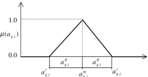
The uncertain time dependent parameters are represented by fuzzy sets. The degrees of membership func-tions for the fuzzy numbers parameters are deﬁned based on subjective judgments. A symmetric triangular fuzzy number is considered to be a more simplistic shape function as it can be constructed easily from two basic estimates – most possible value and maximum deviation from it [32]. For example, a symmetric trian-gular membership function for a fuzzy setup time~ag;i can be deﬁned by

~ ag;i’amg;ia d g;i¼ ða md g;i ;a m g;i;a mþd g;i Þ ¼ ða l g;i;a m g;i;a r g;iÞ ð17Þ

The right and left extreme values have the lowest likelihood of belonging to the set of possible values, and hence have a null degree of membership½l~aðalg;iÞ ¼l~aðarg;iÞ ¼0. The most likelihood value, which lays exactly at the midpoint between the two bound estimates, posses the highest degree of membership ½l~aðamg;iÞ ¼1. Other values within the span of ~ag;i, will assume a linearly varying membership degree in between 0 and 1. Other fuzzy parameters can also be represented in the same fashion. Fig. 1depicts a symmetric triangular membership function for~ag;i.

Likewise, the fuzzy goal function~zð~xÞcan be deﬁned in terms of two crisp functions for weighted ﬂowtime: ~zð~xÞ ’zm_ð_~_x_Þ_zd_ð_~_x_Þ where zmð~xÞ ¼X K k¼1 XJ j¼1 wkðCmk rkÞ Wk;j; and zdð~xÞ ¼ XK k¼1 XJ j¼1 wkðCdkrkÞ Wk;j ð18Þ

Similarly, the fuzzy solution spacev_fð~xÞshown by Eqs.(7)–(16)can also be deﬁned as a combination of two sets of crisp constraints as described next:

vfð~xÞ ﬃvmð~xÞ vdð~xÞ ð19Þ where v_mð~xÞ ﬃpm_i_;_j¼X G g¼1 qm_g_;_iZg;j 8ij2Xg Sm_b_;_i¼Cm_ð_b_m_;_i_Þ 8i b>mi Sm_b_;₂Pcm j;1þM 1_ð_X b;j1Þb6m2 8j Pm b;i¼ XG g¼1 am g;i:Yg;bþ XJ j¼1 pm i;jXb;j 8i 8b Cm_b_;_i¼Sm_b_;_iþPm_b_;_i 8i 8b cm j;iPC m b;iþM 1_ð_X b;j1Þ 8i 8b 8j Cm_k Pcm j;2Wk;j; j2Xk 8k Cm_k 6_d_k ₈_k Cm maxPC m k 8k Sm_b_;_i;P_bm_;_i;Cm_b_;_i;Cm_k;pm_j_;_i;cm_j_;_iP0 and

(8)

vdð~xÞ ﬃpdi;j¼ XG g¼1 qd g;iZg;j 8i j2Xg ð20Þ Sd_b_;_i¼Cd_ð_b_m_;_i_Þ 8i b>mi Sd_b_;₂Pcd_j_;₁þM1 Xb;j1 b6_m₂ ₈_j Pd b;i¼ XG g¼1 ad g;iYg;bþ XJ j¼1 pd i;jXb;j 8i 8b Cd_b_;_i¼Sd_b_;_iþPd_b_;_i 8i 8b cd_j_;_iPCd_b_;_iþM1ðXb;j1Þ 8i 8b 8j Cd_kPcd_j_;₂Wk;j; j2Xk 8k Cd_k6_d_k ₈_k Cd_maxPCd_k 8k Sd_b_;_i;Pd_b_;_i;Cd_b_;_i;Cd_k;pd_j_;_i;cd_j_;_iP0 ð21Þ

A fuzzy decision is obtained by taking the intersection of the fuzzy objective and the total solution space[4]. When information associated with the objective and the set of constraints is vague, the problem can be for-mulated as a fuzzy goal programming problem of type(22):

Find: ~x

To satisfy: ~zð~xÞ ﬃzmð~xÞ and ~x2v_cð~xÞ [v_fð~xÞ ð22Þ

where~xis a solution vector of decision variables within a feasible solution spacevcð~xÞ [vfð~xÞ, andzmð~xÞrefers to the target value of the fuzzy goal. The symbol‘ﬃ 0in the goal constraint represents the linguistic term ‘about’ and it means that the resulting total weighted ﬂowtime~zð~xÞshould be around the vicinity of the aspi-ration value zm_ð_~_x_Þ_{, with some symmetric deviation}_zd_ð_~_x_Þ_{on both sides. As outlined in Section} ₄_{, the target} value zm_ð_~_x_Þ _{is evaluated by taking the most possible values for the individual time dependent fuzzy} parameters.

4. Solution approach

For the fuzzy integer programming problem (FILP) presented in Section3.2, the imprecise objective func-tion will have a symmetric triangular possibility distribufunc-tion. Its shape funcfunc-tion can be deﬁned in terms of the three vertices: ~zð~xÞ ¼ ðzl_ð_~_x_Þ_;_zm_ð_~_x_Þ_;_zr_ð_~_x_ÞÞ_{. Minimization of} _~_z_ð_~_x_Þ _{is achieved by pushing those three vertices} towards the origin. To this end, the mixed-integer fuzzy programming problem is transformed into an auxil-iary multi objective linear programming (MOLP) problem by converting~zð~xÞinto three interdependent crisp objectives[32]. The simultaneous optimization of the three objectives involves minimizing the most possible valuez1ð~xÞ, maximizing the possibility of obtaining lower objectivez2ð~xÞ, and minimizing the risk of obtaining higher objective valuez3ð~xÞ, as shown in(23):

1.0 0.0 ) (ag,i μ r i g a , l i g a, δ i g a, m i g a, δ i g a,

(9)

Min z1ð~xÞ ¼zmð~xÞ

Max z2ð~xÞ ¼zmlð~xÞ ¼zdð~xÞ Min z3ð~xÞ ¼zrmð~xÞ ¼zdð~xÞ

Subject to: ~x2vcð~xÞ [vdð~xÞ

ð23Þ

wherezd_ð_~_x_Þ_{is the symmetric deviation of the triangular fuzzy number}_~_z_{with respect to the aspiration value}_zm_. Employing the fuzzy decision making of Bellman and Zadeh[4]and Zimmermann[34]fuzzy programming method, the auxiliary MOLP problem can be converted into an equivalent single goal linear programming problem. By solving(23)for each objectivezið~xÞseparately, we can determine the initial values for the positive and the negative ideal solutions. Therefore

zPIS₁ ¼Min zmð~xÞ

zNIS₁ ¼Max zmð~xÞ

zPIS₂ ¼zNIS₃ ¼Max zdð~xÞ

zNIS 2 ¼z PIS 3 ¼Min z d_ð_~_x_Þ ð24Þ

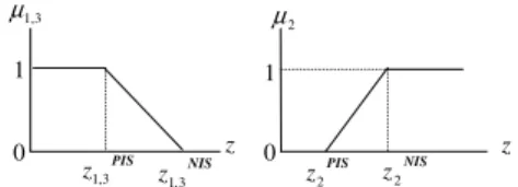
The decision maker can later adjust those parameters interactively within the range of values obtained from (24). The three objective functions are then translated into fuzzy goals using the linear membership functions shown inFig. 2. Equivalently, the three membership functions can be expressed algebraically as in(25):

l₁ðz1Þ ¼ z NIS 1 z1 zNIS 1 z PIS 1 l2ðz2Þ ¼ z2zNIS2 zPIS 2 zNIS2 l3ðz3Þ ¼ zNIS 3 z3 zNIS 3 zPIS3 ð25Þ

Using such linear membership functions and following the fuzzy decision of Bellman and Zadeh[4], the ori-ginal MOLP problem can be interpreted as

Maximize: minfl1ðz1Þ;l2ðz2Þ;l3ðz3Þg

Subject to: ~x2v_cð~xÞ [v_fð~xÞ ð26Þ

By introducing an auxiliary fuzzy goals satisfying levelk ð06_k6₁_Þ_{, the MOLP problem can be reduced to} Zimmermann’s[34]equivalent single objective conventional LP problem:

Maximize: k

Subject to: k6_l

iðziÞ fori¼1;2;3

~x2vcð~xÞ [vfð~xÞ

ð27Þ

Higher value of k (close to 1) indicates that the three objective functions are optimized to a high degree of satisfaction level.

Numerical example-1:A small sized problem consisting of 14 independent job orders from three customers

is considered to demonstrate the approach. Assume, the set of independent jobs can be grouped into four

0 1 PIS 3 , 1 z 3 , 1 μ z NIS 3 , 1 z 0 1 NIS 2 z PIS 2 z 2 μ z

(10)

families based on their style. Two parallel machines are available at each stage of operation. The set of job indices in each group, and the corresponding fuzzy setup and unit processing times are tabulated inTable 1. Employing Eq.(25), the positive and negative ideal solutions for the three objective functions are calculated as follows: zPIS₁ ¼Min zmð~xÞ ¼18 840 zNIS₁ ¼Max zm_ð_~_x_{Þ ¼}_{25 000} zPIS 2 ¼z NIS 3 ¼Max z d_ð_~_x_{Þ ¼}₄₅₀₀

zNIS₂ ¼zPIS₃ ¼Min zdð~xÞ ¼3248

For the equivalent single objective LP model shown in(27), the ﬁnal results are given inTable 2. The auxiliary model is solved using a commercial software LINGO 8.0 installed on a pentium-4 PC, and takes a CPU run-time of 1:35 h. The three auxiliary objective functions are optimized simultaneously with a degree of satisfac-tion levelk¼0:675, bearing the values:z

1¼22 087, andz2¼z3¼4373. As illustrated inFig. 3, the triangular expectation fuzzy number for the imprecise objective ~z is quantiﬁed from the three values. zl_¼_z

1z2¼ 17714;zm_¼_z

1¼22 087 and z

r_¼_z

1þz3¼26 460, which implies that, ~z¼ ðz

l_;_zm_;_zr_{Þ ¼}

Table 1

Example-1: Input data of parameters

Xg Group setup,~ag;i Unit processing,~qg;i

i1 i2 i1 i2 g1 fj3;j4;j11g 25 ± 5 75 ± 15 85 ± 15 230 ± 30 g2 fj2;j5;j10;j14g 15 ± 3 100 ± 25 180 ± 30 260 ± 50 g3 fj1;j6;j9;j13g 20 ± 4 40 ± 10 95 ± 15 325 ± 55 g4 fj7;j8;j12g 30 ± 6 90 ± 12 125 ± 25 410 ± 60 rk¼0 dk¼2500 Wk¼ f0:9;0:7;0:5g Table 2

Example-1: Result output

Xb Batch starting,eSb;i Batch processing,Peb;i Batch completion,Ceb;i i1 i2 i1 i2 i1 i2 b1 fj9g 0 115 ± 19 115 ± 19 365 ± 65 115 ± 19 480 ± 84 b2 fj1g 0 115 ± 19 115 ± 19 365 ± 65 115 ± 19 480 ± 84 b3 fj3;j4;j11g 115 ± 19 480 ± 84 280 ± 50 765 ± 105 395 ± 69 1245 ± 189 b4 fj6;j13g 115 ± 19 480 ± 84 210 ± 34 690 ± 120 325 ± 53 1170 ± 247 b5 fj2;j5g 395 ± 69 1245 ± 189 375 ± 63 620 ± 125 770 ± 132 1865 ± 314 b6 fj7;j8;j12g 325 ± 53 1170 ± 247 405 ± 81 1320 ± 192 730 ± 134 2490 ± 439 b7 fj10;j14g 770 ± 132 1865 ± 314 375 ± 63 620 ± 125 1145 ± 195 2485 ± 439 k¼0:6754 ~z_¼_{22 087}₄₃₇₃ _C_e max¼2500450 ) (x z 1.0 0.0 17714 )) ( (z x μ 4373 4373 26460 22087

(11)

ð17 714;22 087;26 460Þ. Since the shape function for the fuzzy output~zis continuous and symmetric, the most likely valuezm_¼_{22 087 can be considered as the defuzziﬁed value of the imprecise total ﬂowtime.}

5. GA based solution procedure

GA is a population based heuristic search algorithm that mimics the process of evolution and heredity in nature. It follows the principles of’survival of the fittest’ in natural selection to search for best fit individuals within the solution space. In the algorithm, the solution of the problem is coded as a string structure called chromosome. In order to arrive at a near-optimal solution, GA begins searching from a set of randomly gen-erated chromosomes called initial population and evolves to better sets of solutions over a sequence of itera-tions. Each chromosome in the population is evaluated and assigned a fitness value. Fitness value is a measuring criterion for the aptness of the objective function value. Whence, they are directly proportional to each other for the case of a maximization problem, and inversely proportional for the case of a minimiza-tion problem. The higher the fitness value, the better the individual chromosome would be. The search for good chromosomes is guided by the value of the objective function (or fitness measure) for each chromosome in the population [7,16,20].

In GA, one complete-iteration is often referred as a generation. In a given generation, individual chromo-somes within the population will undergo a series of genetic operations and strive for survival to the next gen-eration. Consequently, new chromosomes called oﬀspring with better ﬁtness evolve from the genetic processes. A parent selection mechanism is applied to choose individuals from the current population to a mating poll. Selected individuals in the mating poll reproduce by exchanging genetic materials in a process called crossover operation. Some other chromosomes are also selected to undergo a genetic process called mutation in which only certain parts of their genes are altered to bear a new chromosome. Mutation operators maintain popu-lation diversity by slight perturbations of selected solutions[10,21].

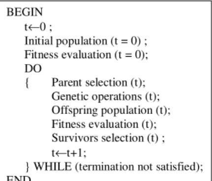
Finally, set of individuals which will pass to the next generation are chosen by employing a survivor selec-tion mechanism. The fittest chromosomes should have a greater chance of being selected in the process. Once an initial population has been created, parent selection, genetic operations, and survivor selection are per-formed sequentially in each generation until it converges to the optimal solution or a stopping criterion is met. This procedure is demonstrated by the pseudo-code shown inFig. 4. For further understanding of the algorithm, we recommend to Ref. [13]. The solution of decision variables in the original problem is then obtained by decoding the best individual chromosome of the final generation. The effectiveness of the GA greatly affected by the proper choice of the chromosomal encoding scheme, parent and survivor selection mechanisms and by the parametric values of crossover and mutation operators[10,22].

5.1. Solution representation (encoding scheme)

In a family setup batch scheduling problem, jobs are ﬁrst sorted into families manually according to their setup similarity. Next, successive decisions of batching and sequencing are made in two phases. Whence, two

BEGIN t←0 ; Initial population (t = 0) ; Fitness evaluation (t = 0); DO { Parent selection (t); Genetic operations (t); Offspring population (t); Fitness evaluation (t); Survivors selection (t) ; t←t+1;

} WHILE (termination not satisfied); END

(12)

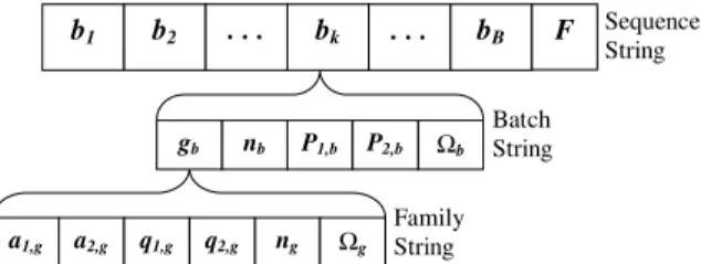
groups of decision variables represent a solution structure – variables for batching decisions, and variables for a sequencing decision. The batching decision variables are used to identify the jobs that are included in each batch from the same family group, while the sequencing decision variables determine the order by which the batches are processed. Therefore, the chromosomal encoding scheme consists of structured information for these two parts: an outer string for the ordering of the batches and an inner string for the creation of each batch.

A path representation using an array of batch indices is the most efficient and widely implemented encoding scheme for the sequencing decision[5,10,13,16]. As shown inFig. 5, the vector of batch indicesfb1;b2;. . .;bBg in the sequencing-string imply that the whole set of jobs available are grouped intoBbatches, and each batch is ordered according to its index value.Fcorresponds to the objective function (i.e., the total weighted flow-time) value for a given solution. It is computed by taking the weighted sum of the elapsed times between receiving and fulfilling of all orders accommodated within the planning horizon. Embedded within each batch, we will find a detail information on how the batch is created. Associated with a given batch bk, a batching string tells the number of jobsðnb6ngÞand set of their indices includedðXb#XgÞ, index key of their family groupðg_bÞ, and the batch-processing times on both machinesðP1;b andP2;bÞ. Through the family index key

ðg_bÞ, the batching string retrieve speciﬁc data pertaining to that family from the input database. The family string data consists of group setup time on the two machinesða1;g anda2;gÞ, unit processing time of a single job on both machines ðq₁_;_g andq₂_;_gÞ, total number of jobs ðngÞ and corresponding set of job indices ðXgÞ within that family. The batch-processing time on both machines can be calculated by the following equation:

Pi;b¼ai;bþ

X

j2Xb

wjqi;b fori¼1;2 ð28Þ

wherewjrefers to the weighting factor of jobj.

5.2. Fitness evaluation

Before a fitness value is assigned, the total weighted flowtime corresponding to each chromosome in the current population must be evaluated. For a given solution representation, the batches will be processed at stage-I according to the order of the batching indices in its sequencing-string. As shown in Fig. 6, batchb1 will be assigned to available first machine,b2to second machine and so on. Once all parallel machines are fully loaded, the rest of the batches, which are not yet assigned, will keep waiting in Line-I until one or more of the machines are freed once again. The batches which are processed on one of the machines at stage-I, will join a second waiting line according to their earliest finish time. At stage-II, the batches are processed according to their lineup sequence in waiting Line-II. Since the setup and processing time of each batch is variable, the resulting sequence in Line-II could probably be different from that of Line-I. This will avoid unnecessary restriction by a permutation sequencing rule which might be imposed only for the sake of simplifying the prob-lem. After the batches complete their processing at stage-II, the jobs within each batch will be re-sorted into their customer groups:k1;. . .;km. After obtaining the completion time of all batches at stage-II, from the sim-ulation process, the total weighted flowtime is computed by the following equation:

F ¼X K k¼1 nkðckrkÞwk where ck ¼ fmaxðcjÞ:8j2Xkg ð29Þ b1 b2 . . . bk . . . bB a1,g a2,g q1,g q2,g ng Ωg gb nb P1,b P2,b Ωb Family String Sequence String Batch String F

(13)

After the objective function (i.e., total flowtime) value is computed for each member of the population, an equivalent fitness value fi, which reflects the relative importance of the individual solution in its domain, is assigned. Since our objective is to minimize the total flowtime, a member with the lowest objective value should correspond to the highest fitness value and vice versa. Therefore, for each chromosome i, its fitness valuefican be evaluated by taking a factorKtimes the reciprocal of the objective function valueFi:

fi¼

K Fi

fori¼1;. . .;N andK ¼constant ð30Þ

5.3. Initial population

The initial population consists ofNrandomly generated chromosomes, whereNstands for the population size. As illustrated in Fig. 7, the chromosomes are created by using either of the two methods – a random batching or a random sequencing heuristic. Primarily, a total of 2 N individuals are generated, and their ﬁtness values be evaluated. Then, the bestNchromosomes out of the total will be chosen to form the initial population. Each member of the initial population are then treated with unary mutation operators joining the evolution cycle. . . ., b6 , b5 , b4 . . ., b’5 , b’4 M-II1 M-II3 M-II2 M-I1 M-I2 M-I3 b1 b2 b3 b’1 b’2 b’3 k1, k2, k3, . . . km Line-I Line-II

Stage-I Stage-II Customer

Grouping

Fig. 6. Queuing simulation of the production ﬂow.

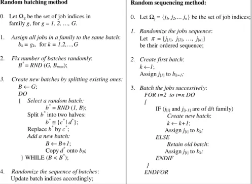
Random batching method

0. Let Ωgbe the set of job indices in

family g, for g = 1, 2, …, G.

1. Assign all jobs in a family to the same batch: bk = gk, for k = 1,2,…,G

2. Fix number of batches randomly: B* = RND(G, Bmax);

3. Create new batches by splitting existing ones: B←G;

DO

{ Select a random batch: b*= RND (1, B); Split b*into two halves:

b*_≅_{_c* _|_d*_};

Replace b* byc*; Add a new batch: B←B+1; Copyd*_onto_b

B;

} WHILE (B < B*_);

4. Randomize the sequence of batches: Update batch indices accordingly;

Random sequencing method:

0. Let Ωj= {j1, j2,… jn} be the set of job indices;

1. Randomize the jobs sequence: Let π = {j[1], j[2], …, j[n]}

be their ordered sequence; 2. Create first batch:

k ←1;

Assignj[1] tobk=1;

3. Batch the jobs successively: FOR i=2 to i=n DO {

IF (j[i]and j[i-1]are of d/t family)

Create new batch: k ←k+1; Assignj[i] tobk;

ELSE

Retain old batch: Assignj[i] tobk;

ENDIF }

ENDFOR

(14)

5.4. Recombination (crossover operation)

Crossover is a binary operation which combines genetic information from two randomly selected parent chromosomes with the purpose of breeding better offspring chromosomes. It exchanges the genetic material of the two parents in order to produce one or two new members for the next generation. The exchange of genes in the process is intended to search for better individuals that improve the good properties of their par-ents[10]. To perform crossover, two parents are selected from the mating pool at random. In order to allow better individuals to become parents of the next generation, up to 5% of the best members are included in the mating poll automatically while the remaining 95% of the population compete with equal selection probability ofp_c. Once a crossover operation has been performed on two mating parents, the new offspring chromosome may be accepted if its fitness is not inferior to that of the worst member in the current population (i.e., Fi<Fmax). Since different number of batches can be created in each parent chromosome, the crossover oper-ators we have considered treat the genes at the detail job string level. At each stage of operation, the processing time of every job in a batch is somehow equal. Therefore, jobs within a batch are arranged based on the ear-liest due date (EDD) sequencing rule.

In our implementation of GA, we have utilized three diﬀerent problem speciﬁc chromosome operations as shown next.

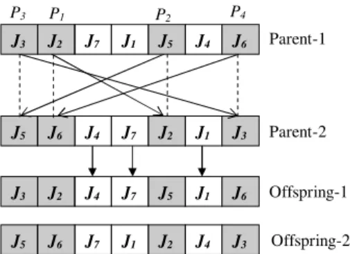
Job based uniform crossover (JUXO): The operator works as follows:

(1) Select two parent chromosomes from the mating poll.

(2) For each parent, extract the jobs included in each batch and build a job based string.

(3) Choose two randomly selected positionsP1 andP2, and block the segment of jobs in between. (4) Copy the blocked jobs from parent-1 to oﬀspring-1 in their respective positions.

(5) From the string of jobs in parent-2, select a job in order, which is not a member of the blocked segment in parent-1 and copy to the lowest vacant position of oﬀspring-1.

(6) For the resulting string in oﬀspring-1, batch adjacent jobs together if they belong to the same family, or separately otherwise.

(7) Update all the genetic information in oﬀspring-1 accordingly.

(8) Reversing the roles of parent-1 and parent-2, repeat from step 4 to create oﬀspring-2.

Example. Suppose the string of jobs in the two mating parents be fJ3;J2;J7;J1;J5;J4;J6gand fJ5;J6; J4;J7;J2;J1;J3g, respectively, as shown inFig. 8. IfP1 andP2are randomly chosen to be the second and fifth positions, we shade all jobs fromP1 toP2 inclusive. Next, the shaded jobs from each parent are copied to the same location of boxes in the two offsprings. To fill out the empty boxes of offspring-1, we look into the sequence of jobs in the second string and vice versa. The first potential candidate from the second string to fill out the left most empty box of offspring-1 isJ5. SinceJ5is a member of the shaded segment in offspring-1, it fails to satisfy the selection criteria. Moving forward one more step along the same string, we findJ6. SinceJ6 is not included in the shaded part of 1, it will be eligible to be placed at the first position of offspring-1. Next we findJ4, which satisfies the criteria to fill out the second vacant box. Continuing the process in the

J1 J2 J7 J4 J3 J5 J6 J1 J4 J7 J2 J3 J5 J6 J1 J4 J7 J2 J6 J5 J3 J5 J4 J7 J2 J6 J3 J1 Parent-1 Parent-2 Offspring-2 Offspring-1 P1 P3 P2

(15)

same way, we will get J2 andJ3 that can meet the selection condition to fill out the two remaining vacant boxes, respectively. Likewise, the empty boxes in offspring-2 are filled by copying unscheduled job indices from the first string, which are not members of the shaded block in parent-2.

Job based cyclic crossover (JCXO):This operator works as follows:

(1) Repeat steps 1 and 2 of JUXO. (2) Constrict the cycle as follows:

(a) Start with a randomly selected job position P1 from parent-1. (b) Include P1 in the cycle and record the corresponding job.

(c) Find a new position Piindicating the recorded job in parent-2. (d) AddPi to the cycle and record the corresponding job in parent-1.

(e) Repeat steps (c) and (d) if Pi–P1.

(3) For the corresponding positions in the cycle, copy the indicated jobs from parent-1 to oﬀspring-1 in their respective places.

(4) Select the unscheduled jobs from the string in parent-2, and copy them into the vacant positions of oﬀ-spring-1 sequentially.

(5) Batch adjacent jobs in the string of oﬀspring-1 together if they belong to the same family, or separately otherwise.

(7) For the case of oﬀspring-2, repeat the steps from 3 to 6 by swapping the tasks of the two parents.

Example. As illustrated in Fig. 9, suppose the string of jobs in the two mating parents be the same as the previous example. Let the second position be our first point P1 to start the cycle. In the first string, P1 indicates to the position of J2. Then, we look for the position of J2 in the second string (i.e., to fifth position) and fix point P2. Since P2 points to J5 in the first string, we search for J5 in parent-2 and fix point P3. In the same way, P4 is shown by looking to the position of J3 in the second string. The job represented by P4 in parent-1 is J6. Continuing the search for J6 in parent-2, we will rest on the second position, which corresponds to our initial point P1. At this point, we terminate our search for new positions as the cycle will repeat itself. Next, we shade all the jobs inside the boxes pointed out by points P1;P2;P3 andP4. The shaded jobs from each parent are then copied to the two offsprings in their respective locations. The remaining task is to fill out the empty boxes in each offspring by pasting unscheduled jobs sequentially from the string of jobs in the other parent, as we did in the previous example.

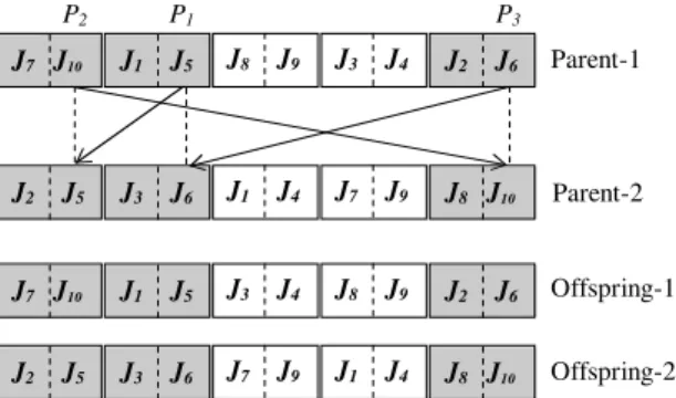
Batch based cyclic crossover (BCXO): This operator works as follows:

(1) Repeat steps 1 and 2 of JUXO.

J1 J4 J7 J2 J3 J5 J6 Parent-2 J1 J2 J7 J4 J3 J5 J6 Parent-1 P1 P2 P4 P3 Offspring-1 J7 J2 J4 J1 J3 J5 J6 Offspring-2 J4 J7 J1 J2 J3 J5 J6

(16)

(2) Constrict a batch based cycle as follows:

(a) Choose a starting positionP1randomly from parent-1, add it to the cycle and record the indicated job.

(b) Mark those jobs aroundP1which belong to the same batch. (c) Find a new positionPi in parent-2 containing the recorded job. (d) Mark those jobs aroundPiwhich belong to the same batch.

(e) AddPito the cycle and record the corresponding job in parent-1. (f) Repeat steps (c) to (e) untilPi rests on any marked job in parent-1.

(3) Copy all marked jobs from parent-1 and paste to their own places in oﬀspring-1.

(4) Select unscheduled jobs sequentially from the string in 2, and copy the batch of jobs from parent-1 into the lowest vacant position(s) of oﬀspring-parent-1.

(5) In the job sequence for oﬀspring-1, batch adjacent jobs together if they belong to the same family, or separately otherwise.

(7) To create oﬀspring-2, repeat from step 3 by exchanging the roles of the parents.

Example. Suppose the two parents contain 10 jobs which are grouped into five batches. In the sequencing-string, the jobs belonging to the same batch are bounded by the smaller boxes as shown inFig. 10. Let our starting pointP1be at the position ofJ5in parent-1. In order to locateP2, we search for the location ofJ5in the second string and shade the entire batch containingJ₅in both parents. The job indicated byP₂in the first string isJ10. Therefore, we look into the position ofJ10in parent-2 to fix pointP3and shade the corresponding batches. UnderP3 isJ6 which will direct us to the starting pointP1 in the second string. After shading the batches containingJ6 in both parents, we terminate the cycle. All shaded batches from each parent are then copied to the offsprings as they are. To complete offspring-1, we look for the unscheduled jobs in the second string. Since J3 is not scheduled in offspring-1, we copy the batch containing J3 from parent-1 to the left vacant positions. The two remaining empty boxes in offspring-1 are then filled by copying the last batch containing J4 from parent-1. Likewise, the empty boxes in offspring-2 are filled by copying batches from parent-2, based on the sequence of unscheduled jobs in the first string.

5.5. Mutation

Mutation operators are mainly used to prevent premature convergence. Mutation is also used to make local searching around a given solution, or to reintroduce lost genetic material and variability in the population. This operator can also be seen as a simple form of local search. Mutation is a way of enlarging the search space. It acts to prevent the selection and crossover from focusing on a narrow area of the search space or from the GA getting stuck in a local optimum. By mutating an individual, we slightly alter the chromosome,

P1 J1 J5 J8 J9 J3 J4 J2 J6 J7 J10 J2 J5 J3 J6 J1 J4 J7 J9 J8 J10 J1 J5 J3 J4 J8 J9 J2 J6 J7 J10 J2 J5 J3 J6 J7 J9 J1 J4 J8 J10 Parent-1 Parent-2 Offspring-1 Offspring-2 P2 P3

(17)

thus allowing a new but similar permutation. After undergoing mutation, if the fitness value improves, then the mutated individual will automatically replace its parent. However, if its fitness is less than that of the par-ent but still higher than the worst member of the population, then it will be allowed to join the currpar-ent pop-ulation as a new offspring chromosome. On the contrary, if the fitness of the mutated individual is less than the worst fitness member, it will be rejected automatically at its time of birth. Mainly three different mutation operators are proposed in the literature for permutation encodings: Swap, Position, Shift [21,10]. We have implemented a number of mutation operators in our application of GA:

FLIP mutation: Here, the sequencing-string of a member is partitioned into two parts at a randomly chosen location. The block of batches in the second portion are then cut from the string and placed in front of the ﬁrst portion. Next, all genetic information in the modiﬁed individual is updated accordingly.

SWAP mutation: Two batch positions are chosen randomly from the sequence-string of a member. The

genetic material within the two batches is then exchanged giving a variation to the original chromosome.

SHIFT mutation: In this case, a batch at a randomly chosen position is picked from a sequence-string and relocated adjacent to another randomly picked position, causing the string of batches in between to be dis-placed by one step in the reverse direction. The genes are then updated accordingly.

SHUFFLE mutation: This works by choosing two positions from the sequencing-string of a member at

ran-dom. The orders of batches in between the two positions are then randomized, and their genes modiﬁed accordingly.

INVERT mutation: This also works by randomly picking two positions in the entire string of a member and reversing the order of the batches in between the two positions.

MERGE mutation: In this case, families of jobs, which are divided into two or more batches, are first iden-tified for a given member. Then, two batches containing jobs from a randomly chosen family are selected. Giving all of its genes to the first batch, the second batch destroys itself in the process and pulls the block of batches after it by one step. The genetic information of the variation member is then updated.

SPLIT mutation: Here, a randomly picked batch consisting of two or more jobs is selected from a sequence-string of a member. Its genes are then divided into two parts with random sizes. The ﬁrst part replaces the original batch while the second part introduces a new batch positioned at the end of the string.

WSPT-mutation: Here the problem is ﬁrst conceived as a single machine ﬂowtime problem and the batches

in the entire string are arranged by a weighted shortest processing time (WSPT) rule. This sequencing rule minimizes optimally the weighted ﬂowtime of independent jobs for the case of one-machine problem with-out a setup. In order to combine the processing time of each batch at the two stages, the operator intro-duces a parameter. The operator works as follows:

(1) For a given member, letX¼ fb1;b2;. . .;bBg be the set of batches in the sequence-string. (2) Select a random value ofawhere 06_a6_1.

(3) For each batch, calculate the combined processing time by:Pb¼aP1;bþ ð1aÞP2;b for8b2X. (4) Arrange the batches in increasing order ofPb.

(5) Modify the genes in the variation chromosome accordingly.

JOHNSON mutation: This operator follows a modiﬁed Johnson’s heuristic to alter the sequencing-string of a member. The classical Johnson’s algorithm optimally minimizes the makespanðCmaxÞof independent jobs for the case of two-machine ﬂowshop problem without a setup. The operator works as follows:

(1) Let X¼ fb1;b2;. . .;bBg be the set of batches in the sequence-string.

(2) Partition X in two subsets (U and V) based on the dominant processing time:

U¼ fb2X:P1;bPP2;b andV ¼ fb2X:P1;b<P2;bfor8b2X.

(18)

(4) Append the block of batches inVnext to those inUto get a complete string. (5) Update the genes in the member accordingly.

ADOPT mutation: This operator simply introduces a randomly created chromosome to the current

popula-tion. Its operation is conditioned to the gab between the objectives of the best and worst chromosomes in the current population. When the gab gets smaller and smaller at higher generations, the operator introduces a new chromosome to replace the worst member. It basically helps to improve population diversity in the com-ing generations by allowcom-ing more chromosomes to survive.

Repeated execution of the GA simulation reveals that, the crossover operators considered are more eﬃcient at lower generations while the mutation operations are more eﬃcient at higher generations. However, the rel-ative importance of each operator varies from one problem instant to another.

5.6. Survivor selection mechanism

The population size from generation to generation is supposed to be constant. Thus, survivor selection mechanism is used to choose the set of individuals from the current parent and offspring population, which are allowed to exist in the next generation. We basically implemented a combination of two well known strat-egies in order to decide whether a member has to live or die. Among the survivor population,PE%are selected using a biased (Elitist) mechanism in which only the best fit chromosomes are chosen. The remaining 1PE% of the survivors are then selected by a fitness proportional (Roulette wheel) mechanism. The parameterPE%, which controls the boundary between the two strategies, can be referred as ‘degree of elitism’.

5.7. Termination criterion and parameters tuning

The control parameters which affect the efficiency of GA are: the population sizeN, the parent selection probabilityp_c in the mating poll to undergo a crossover operation, and the probability of mutation p_m. In our implementation of GA, if the best fitness level cannot improve after 200 additional generations, we will terminate the algorithm. For a given problem input data, we execute the algorithm with assigned parametric values and record the best solution obtained, the CPU runtime and maximum generation. In order to ensure that the GA is not trapped by local optima, we repeat the numerical simulation with different set of values of the control parameters (i.e., population size, operators’ probability, degree of elitism, etc.) and record the best solution obtained from the experiment. From our design of experiment (DOE), we observe that the parame-ters are insensitive for a wide interval of values proving the GA to be robust.

Numerical example-2: We considered a medium-sized problem with 60 jobs and 10 family groupings. The

job orders came from six equally valued customers. Based on their customer-ID, the jobs are indexed as follows: X1¼ fJ1;. . .;J12g;X2¼ fJ13;. . .;J23g;X3¼ fJ24;. . .;J36g;X4¼ fJ37;. . .;J45g;X5¼ fJ46;. . .;J52g; andX6¼ fJ53;. . .;J60g. The set of job indices in each family group and along with their fuzzy setup and unit

Table 3

Example-2: Data of input values

Indexg Setup time Unit processing time Set of jobs per familyg:Xg

~ a1;g ~a2;g ~q1;g ~q2;g ½1 46124 76634 33723 53838 fJ32g ½2 32733 82525 29330 37037 fJ10;J13;J18;J25;J28;J31;J33;J36;J39;J48;J50g ½3 27228 64232 23424 54735 fJ57g ½4 49825 98727 31231 44342 fJ7;J9;J17;J20;J29;J30;J41;J45;J59;J60g ½5 31224 75222 28723 36836 fJ4;J16;J19;J35;J42;J43;J44;J51;J52;J58g ½6 22332 81218 37727 38643 fJ1;J3;J6;J8;J12;J14;J34;J37;J53;J54;J55g ½7 34725 85023 26136 53939 fJ2;J5;J38;J56g ½8 47828 79234 37928 46844 fJ22g ½9 32223 73828 28535 54439 fJ11;J21;J23;J24;J27;J40;J46;J47;J49g ½10 28521 87824 29125 39949 fJ15;J26g

(19)

processing times is given in Table 3. The production setup consists of two and three identical machines at stage-1 and stage-2, respectively.

Using the most possible values for the imprecise setup and processing times, we tested the GA for about 20 times with diﬀerent set of control parameters. Accordingly, we select the following combination of parameters in solving the problem: population size Np¼100, crossover probability pc¼0:15, mutation probability: p_m¼0:1, and percentage of elitist selectionPE¼50%. The best incumbent solution is obtained after 500 cycles of generations. The resulting sequence batches and the job indices included in each batch are tabulated in Table 4. To account for the fuzziness of the objective function, next we determine its deviation from the mean by re-evaluating the incumbent solution using the maximum deviation values of the setup and processing times. Finally, we found the imprecise total ﬂowtime to be F ’675 70658 270. The GA is executed on a Pentium(R)4 PC with 3 GHz speed and 1 GB RAM, and took a CPU runtime of 4:27 min to converge.

The proposed GA has been tested for diﬀerent problem instances and the results obtained are compared with the LINGO solution. For all cases, the mean values of the setup and unit processing time vary uniformly over the intervals indicated in Table 5. Considering the most likelihood value zm _{to compare the} two approaches, Table 6 shows summary of results obtained for 10 diﬀerent instances of problems. The

Table 4

Example-2: Batches created according to their sequence of operations Set of jobs per batchb:B½b¼Xb

B½1¼ fJ10;J13g B½10¼ fJ22g B½2¼ fJ2;J5;J38;J56g B½11¼ fJ24;J27;J40g B½3¼ fJ11;J21;J23g B½12¼ fJ32g B½4¼ fJ1;J3;J6;J8;J12g B½13¼ fJ41;J45;J59;J60g B½5¼ fJ7;J9;J17;J20;J29;J30g B½14¼ fJ43;J44;J51;J52;J58g B½6¼ fJ4;J16;J19;J35;J42g B½15¼ fJ46;J47;J49g B½7¼ fJ15;J26g B½16¼ fJ54;J55g B½8¼ fJ18;J25;J28;J31;J33;J36;J39;J48;J50g B½17¼ fJ53g B½9¼ fJ14;J34;J37g B½18¼ fJ57g Table 5

Range of values for the input parameters

Parameter Range of values

Setup time at stage-I,a1 (200, 500)

Setup time at stage-II,a2 (800, 1200)

Unit processing time at stage-I,q1 (100, 400)

Unit processing time at stage-II,q2 (500, 1000)

Table 6

Comparison of results for diﬀerent problem instances

PR. code Test problem size Best solutionð 106Þfound and CPU runtime (s)

JobsJ GroupsG OrdersK Machines GA LINGO

m1 m2 F ’zm Time F’zm LB Time T1 5 2 2 1 2 0.0209 6.86 0.020901a 0.020901 7 s T2 10 3 2 2 2 0.0588 13.75 0.060655 0.030925 2.5 h T3 25 5 4 2 3 0.2029 34.06 0.224751 0.015642 1 h T4 50 10 6 2 4 0.5875 95.09 0.727642 0.029242 12 h T5 75 15 7 3 4 1.2415 240.05 · · · T6 100 18 10 3 5 1.7665 145.75 · · · T7 150 25 12 4 6 2.9734 331.69 · · · T8 200 30 15 5 8 4.3141 1508.83 · · · T9 250 32 20 6 10 4.8936 1364.39 · · · T10 300 35 25 10 15 4.9653 5494.22 · · ·

·= problem oversized to be solved by LINGO.

a

(20)

computational experiment conﬁrms that the proposed GA gives better quality of solution with medium com-putational eﬀort especially for larger problem sizes.

6. Conclusion

In this paper, we have demonstrated a mixed-integer fuzzy programming (MIFP) approach for batch scheduling of jobs on parallel machines in a two-stage flowshop. The goal of the fuzzy model is to improve customer responsiveness by reducing the total weighted flowtime for all jobs in the system. The fuzzy math-ematical programming approach incorporates the uncertainties associated with estimation of time dependent parameters directly into the optimization model. Such representations of fuzzy parameters with membership functions avoid the need to perform sensitivity analysis after an optimal solution is obtained. The uncertainty associated with batch-processing and setup times are represented by triangular fuzzy sets. Numerical results demonstrate that the proposed model can efficiently schedule small size of jobs. While for higher number of jobs, a robust GA solution method is suggested. The proposed model is vital as a sound decision support tool in the practical application of furniture scheduling, especially when the processing and setup times cannot be determined precisely.

References

[1] G.I. Adamopoulos, C.P. Pappis, N.I. Karacapilidi, Job sequencing with uncertain and controllable processing times, Int. Trans. Op. Res. 6 (1999) 483–493.

[2] A. Allahverdi, J.N.D. Gupta, T. Aldowaisan, A review of scheduling research involving setup considerations, Omega, Int. J. Manage. Sci. 27 (1999) 219–239.

[3] J. Balasubramanian, I.E. Grossmann, Scheduling optimization under uncertainty: an alternative approach, Comput. Chem. Eng. 27 (2003) 469–490.

[4] R.E. Bellman, L.A. Zadeh, Decision-making in a fuzzy environment, Manage. Sci. 17 (1970) 141–164.

[5] R.L. Burdett, E. Kozan, Evolutionary algorithms for ﬂowshop sequencing with non-unique jobs, Int. Trans. Op. Res. 7 (2000) 401– 418.

[6] S. Chanas, A. Kasperski, On two single machine scheduling problems with fuzzy processing times and fuzzy due dates, Eur. J. Oper. Res. 147 (2003) 281–296.

[7] P. Damodaran, P.K. Manjeshwar, K. Srihari, Minimizing makespan on a batch-processing machine with non-identical job sizes using genetic algorithms, Int. J. Product. Econ. (2006).

[8] P. Damodaran, K. Srihari, Mixed integer formulation to minimize makespan in a ﬂow shop with batch processing machines, Math. Comput. Model. 40 (2004) 1465–1472.

[9] T. Itoh, H. Ishii, Fuzzy due-date scheduling problem with fuzzy processing time, Int. Trans. Op. Res. 6 (1999) 639–647.

[10] S.K. Iyera, B. Saxena, Improved genetic algorithm for the permutation ﬂowshop scheduling problem, Comput. Oper. Res. 31 (2004) 593–606.

[11] M.M. Liaee, H. Emmons, Scheduling families of jobs with setup times, Int. J. Product. Econ. 51 (1997) 165–176. [12] M. Litoiua, R. Tadeib, Fuzzy scheduling with application to real-time systems, Fuzzy Sets Syst. 121 (2001) 523–535. [13] Z. Michalewicz, Genetic Algorithms + Data Structures = Evolution programs, third ed., Springer-Verlag, Berlin, 1996.

[14] E. Nowicki, C. Smutnicki, The ﬂow shop with parallel machines: a tabu search approach, Eur. J. Oper. Res. 106 (1998) 226–253. [15] J. Peng, B. Liu, Parallel machine scheduling models with fuzzy processing times, Inf. Sci. 166 (2004) 49–66.

[16] M.C. Portmann, A. Vignier, D. Dardilhac, D. Dezalay, Branch and bound crossed with GA to solve hybrid ﬂowshops, Eur. J. Oper. Res. 107 (1998) 389–400.

[17] C.N. Potts, M.Y. Kovalyov, Scheduling with batching: a review, Eur. J. Oper. Res. 120 (2000) 228–249.

[18] C. Rajendran, H. Ziegler, Scheduling to minimize the sum of weighted ﬂowtime and weighted tardiness of jobs in a ﬂowshop with sequence-dependent setup times, Eur. J. Oper. Res. 149 (2003) 513–522.

[19] R. Ruiz, C. Maroto, A comprehensive review and evaluation of permutation ﬂowshop heuristics, Eur. J. Oper. Res. 165 (2005) 479– 494.

[20] R. Ruiz, C. Maroto, A genetic algorithm for hybrid ﬂowshops with sequence dependent setup times and machine eligibility, Eur. J. Oper. Res. 169 (2006) 781–800.

[21] R. Ruiz, C. Maroto, J. Alcaraz, Two new robust genetic algorithms for the ﬂowshop scheduling problem, Omega 34 (2006) 461–476. [22] R. Sarker, C. Newton, A genetic algorithm for solving economic lot size scheduling problem, Comput. Ind. Eng. 42 (2002) 189–198. [23] T. Sawik, Integer programming approach to production scheduling for make-to-order manufacturing, Math. Comput. Model. 41

(2005) 99–118.

[24] A. Sharma, P. LaPlaca, Marketing in the emerging era of build-to-order manufacturing, Ind. Market. Manage. 34 (2005) 476–486. [25] J.M.J. Schutten, R.A.M. Leussink, Parallel machine scheduling with release dates, due dates and family setup times, Int. J. Product.

(21)

[26] X. Wang, T.C.E. Cheng, Two-machine ﬂowshop scheduling with job class setups to minimize total ﬂowtime, Comput. Oper. Res. 32 (2005) 2751–2770.

[27] C.-S. Wang, R. Uzsoy, A genetic algorithm to minimize maximum lateness on a batch processing machine, Comput. Oper. Res. 29 (2002) 1621–1640.

[28] C. Wang, D. Wang, W.H. Ip, D.W. Yuen, The single machine ready time scheduling problem with fuzzy processing times, Fuzzy Sets Syst. 127 (2002) 117–129.

[29] A.D. Wilson, R.E. King, T.J. Hodgson, Scheduling non-similar groups on a ﬂow line: multiple group setups, Rob. Comput.-Integr. Manuf. 20 (2004) 505–515.

[30] D.L. Yang, M.S. Chern, Two-machine ﬂowshop group scheduling problem, Comput. Oper. Res. 27 (2000) 975–985. [31] A.C. Yao, J.G.H. Carlson, Agility and mixed-model furniture production, Int. J. Product. Econ. 81–82 (2003) 95–102.

[32] A.D. Yimer, K. Demirli, Minimizing weighted ﬂowtime in a two-stage ﬂow shop with fuzzy setup and processing times, in: North America Fuzzy Information Processing Society (NAFIPS-06) Annual Meeting, IEEE Conference Proceeding, 2006, pp. 708–713. [33] S. Zdrzalka, A sequencing problem with family setup times, Discrete Appl. Math. 66 (1996) 161–183.