Semantic Information G Theory and Logical Bayesian Inference for Machine Learning

Information2019, 10, 261; doi:10.3390/info10080261 www.mdpi.com/journal/information Article

Semantic Information G Theory and Logical Bayesian

Inference for Machine Learning

Chenguang Lu

Institute of Intelligence Engineering and Mathematics, Liaoning Technical University, Fuxin 123000, China; [email protected]

Received: 20 June 2019; Accepted: 13 August 2019; Published: 16 August 2019

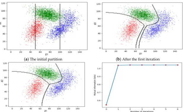
Abstract: An important problem in machine learning is that, when using more than two labels, it is very difficult to construct and optimize a group of learning functions that are still useful when the prior distribution of instances is changed. To resolve this problem, semantic information G theory, Logical Bayesian Inference (LBI), and a group of Channel Matching (CM) algorithms are combined to form a systematic solution. A semantic channel in G theory consists of a group of truth functions or membership functions. In comparison with the likelihood functions, Bayesian posteriors, and Logistic functions that are typically used in popular methods, membership functions are more convenient to use, providing learning functions that do not suffer the above problem. In Logical Bayesian Inference (LBI), every label is independently learned. For multilabel learning, we can directly obtain a group of optimized membership functions from a large enough sample with labels, without preparing different samples for different labels. Furthermore, a group of Channel Matching (CM) algorithms are developed for machine learning. For the Maximum Mutual Information (MMI) classification of three classes with Gaussian distributions in a two-dimensional feature space,only 2–3 iterations are required for the mutual information between three classes and three labels to surpass 99% of the MMI for most initial partitions For mixture models, the Expectation-Maximization (EM) algorithm is improved to form the CM-EM algorithm, which can outperform the EM algorithm when the mixture ratios are imbalanced, or when local convergence exists. The CM iteration algorithm needs to combine with neural networks for MMI classification in high-dimensional feature spaces. LBI needs further investigation for the unification of statistics and logic.

Keywords: semantic information theory; Bayesian inference; machine learning; Multilabel learning; maximum mutual information classifications; mixture models; confirmation measure; truth function

1. Introduction

Machine learning is based on learning functions and classifiers. In 1922, Fisher [1] proposed the Likelihood Inference (LI), which uses likelihood functions as learning functions and it uses the Maximum Likelihood (ML) criterion to optimize the learning functions and classifiers (see Appendix A for all abbreviations in this paper). However, when the prior distribution, P(x) (where x is an instance), is changed, the optimized likelihood function will be invalid. As LI cannot make use of prior knowledge, Bayesians proposed Bayesian Inference (BI) during the 1950s [2,3], which uses Bayesian posteriors as learning functions. However, in many cases, we only have prior knowledge of instances, instead of labels or model parameters and, hence, BI is still not good in such cases. A pair of Logistic (or Sigmoid) functions are often used as the learning functions for binary classifications. With a Logistic function and Bayes’ Theorem, we can make use of a new prior P(x) to make new

probability predictions for the ML classifier. However, when the number of labels is greater than two, we cannot find proper learning functions that are similar to Logistic functions for multilabel learning. We call the above problem the “Multilabel-Learning-for-New-P(x) Problem”.

Machine learning is used to acquire and convey information, and so the information criterion that is used should be a good criterion. In 1974, Akaike [4] proved that the ML criterion is equal to the minimum Kullback–Leibler (KL) divergence criterion, where the KL divergence [5] is also called “KL information”. Since then, information criteria, especially information criteria that are compatible with the likelihood criterion, have attracted the attention of researchers [6]. However, KL divergence decreases as the likelihood increases and, hence, the Least KL divergence is not ideal as an information criterion. Can we use Shannon’s mutual information or another information measure for the information criterion?

In 1948, Shannon [7] initiated classical information theory. In 1949, Weaver [8] proposed three levels of communication that are relevant to the technical problem that was resolved by Shannon, a semantic problem that relates to meaning and truth, and an effectiveness problem concerning information values. In 1952, Carnap and Bar-Hillel [9] proposed an outline of semantic information theory. Multiple different semantic information theories currently exist [10–13], as well as fuzzy information theories [14–16] and generalized information theories [17,18] that are related to semantic information theories. Recently, some researchers have used the Shannon mutual information measure with parameters to optimize neural networks [19,20].

However, Shannon’s Mutual Information (SHMI) formula has not yet been used to optimize a learning functions with parameters by the use of a sampling distribution. Therefore, the author introduced a learning function into the SHMI formula and developed semantic information G theory, or G theory. The author mainly developed this theory over the past three decades [21–26]. The G theory uses the membership functions of fuzzy sets, as proposed by Zadeh [27], as learning functions and treats a membership function as the truth function of a hypothesis. The truth function can represent the semantic meaning of a hypothesis, according to Tarski’s truth theory [28] and Davidson’s truth-conditional semantics [29].

“G theory” is used because, in this theory, Semantic Mutual Information (SMI) is a natural generalization of SHMI (“G” denoting “generalization”), so that SHMI is the upper limit of SMI. G

also denotes SMI as D denotes average distortion in Shannon’s information rate distortion theory [30]. Replacing D with G, the author reformed the rate-distortion function R(D) into the rate-verisimilitude function R(G) [24,25], not only for data compression, but also for machine learning.

G theory has two headstreams: Shannon’s information theory and Popper’s hypothesis-testing theory (see [31], p. 96 and 269; and [32], p. 294), which emphasizes that a hypothesis with a smaller logical probability can convey more information if it can survive empirical tests and, hence, is more preferable.

Carnap and Bar-Hillel [9] used logical probability to define the semantic information measure, which contains Popper’s partial thought. However, this measure does not deal with whether the hypothesis can survive empirical tests. Therefore, G theory introduces the membership function into the semantic information measure.

Cross-entropy has become a popular tool in machine learning [33]. G theory uses not only cross-entropy, but also mutual cross-entropy [22,25]. The SMI in G theory is a mutual cross-entropy.

To resolve the “Multilabel-Learning-for-New-P(x)” problem, the author investigated a new inference method: Logical Bayesian Inference (LBI). The Bayesians include subjective Bayesians and logical Bayesians. BI was developed by subjective Bayesians, who use subjective probability for statistical inference. Logical Bayesians, such as Keynes and Carnap [34], use logical probability, including the truth function, for inductive logic. BI uses the Bayesian posterior as the inferential tool. Logical Bayesian Inference uses the truth function (e.g., the fuzzy truth function) instead of the Bayesian posterior as the inferential tool. In LBI, both statistical and logical probabilities are simultaneously used. BI fits cases with a given prior distribution of a predictive model θ, whereas LBI fits cases with a given prior distribution of an instance X.

Besides Shannon’s information theory and Poppers’ hypothesis-testing theory, G theory and LBI should inherit, absorb, or be compatible with:

• Fisher’s likelihood method for hypothesis-testing [1];

• Zadeh’s fuzzy set theory [27,35] for semantic meanings and logical probabilities of hypotheses;

• Carnap and Bar-Hillel’s semantic information formula with logical probability [9];

• Floridi’s semantic concepts of information [11,36];

• Tarski’s truth theory for the definition of truth and logical probability [28];

• Davidson’s truth-conditional semantics [29];

• Kullback and Leibler’s KL divergence [5];

• Akaike’s proof [4] that the ML criterion is equal to the minimum KL divergence criterion;

• Theil’s generalized KL formula [37];

• the Donsker–Varadhan representation as a generalized KL formula with Gibbs density [38];

• Wittgenstein's thought: meaning lies in uses (see [39], p.80);

• Bayes’ Theorem [40], which can be extended to link likelihood functions and membership functions [41]; and,

• Logical Bayesian methods for inductive logic used by Carnap et al. [3,34]

Based on G theory and LBI, the author developed a group of algorithms, called Channel Matching (CM) algorithms [41–44], for machine learning. In the CM algorithms, the semantic channel and Shannon channel mutually match to achieve maximum information (for classification) or maximum information efficiency (G/R) (for mixture models).

These algorithms are used mainly for:

• making use of the prior knowledge of instances for probability predictions;

• multilabel learning, belonging to supervised learning;

• the Maximum Mutual Information (MMI) classifications of unseen instances, belonging to semi-supervised learning; and,

• mixture models, belonging to unsupervised learning. Each of them is very difficult and not well resolved before.

This study aims to completely introduce G theory, LBI, and the CM algorithms, along with sufficient background knowledge and applications for readers to fully understand them, especially to understand how to use them to resolve the “Multilabel-Learning-for-New-P(x)” Problem.

Partial contents of this paper have been introduced in several short papers that were published in conference proceedings [41–44]. Some contents introduced before are improved in this paper, such as one-dimensional examples for MMI classification and mixture models, which are now two-dimensional examples, as well as the previous two formulae for the confirmation measure being consolidated into one formula.

According to the author’s knowledge, nowhere in the literature has a semantic information measure been used to optimize the membership functions or truth functions with parameters by sampling distributions; no has the statistical probability and the logical probability of a hypothesis been distinguished and simultaneously used in the same formula; nor has the semantic channel with its mathematical representation been proposed.

2. Methods I: Background

2.1.FromShannonInformationTheorytoSemanticInformationGTheory

2.1.1. From Shannon’s Mutual Information to Semantic Mutual Information

Definition 1.

• x: an instance or data point; X: a discrete random variable taking a value x∈U = {x1, x2, …, xm}. • y: a hypothesis or label; Y: a discrete random variable taking a value y∈V = {y1, y2, …, yn}.

• P(yj|x) (with fixed yj and variable x): a Transition Probability Function (TPF) (named as such by Shannon

[7]).

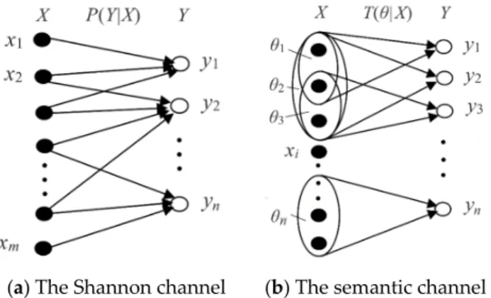
Shannon named P(X) the source, P(Y) the destination, and P(Y|X) the channel. A Shannon channel is a transition probability matrix or a group of transition probability functions:

1 1 1 2 1 2 1 2 2 2 1 2 ( | ) ( | ) ... ( | ) ( | ) ( | ) ( | ) ... ( | ) ( | ) ( | ) ... ... ... ... ... ( | ) ( | ) ... ( | ) ( | ) m j m j n n n m n P y x P y x P y x P y x P y x P y x P y x P y x P Y X P y x P y x P y x P y x             ⇔_{ }⇔_{ }         ， ₍₁₎

where  indicates equivalence. Note that the TPF P(yj|x) is not normalized, unlike the conditional

probability function, P(y|xi), in which y is variable and xi is constant. We will discuss how the TPF

can be used for the traditional Bayes prediction in Section 2.2.1. The Shannon entropies of X and Y are

( )= ( ) log ( ),_{i i} j H X −





The Shannon posterior entropies of X and Y are

( | )= ( ,_{i j}) log ( |_{i j}), j i H X Y −

 

 

The Shannon mutual information is

( | ) ( ; )= ( , ) log ( ) ( | ) ( ) ( | ) ( , ) log ( ) ( | ). ( ) i j i j j i i j i i j j i j P x y I X Y P x y H X H X Y P x P y x P x y H Y H Y X P y − = − = − = −

 

 

If Y=yj, the mutual information I(X;Y) will become the Kullback–Leibler (KL) divergence:

( | ) ( | ) ( ; )= ( | ) log = ( | ) log . ( ) ( ) i j j i j i j i j i i i j P x y P y x I X y P x y P x y P x P y





Some researchers have used the following formula to measure the information between xiand

yj: ( | ) ( | ) ( ; )= log log . ( ) ( ) i j j i i j i j P x y P y x I x y P x = P y (8)

As I(xi;yj) may be negative, however Shannon did not use this formulation. Shannon explained that

information is the reduced uncertainty or the saved average code word length. The author believes that the above formula is meaningful, because negative information indicates that a bad prediction may increase the uncertainty or the code word length.

As Shannon’s information theory cannot measure semantic information, Carnap and Bar-Hillel proposed a semantic information formula

I(p) = log[1/mp]. (9)

Zhong [12] made use of the fuzzy entropy of DeLuca and Termini [14] to define the semantic information measure

I(yj) = log2 + [tj logtj + (1 – tj) log(1 − tj)], (10)

where tj is “the logical truth” of yj. However, according to this formula, whenever tj=1 or tj=0, the

information reaches its maximum of 1 bit. This result is not expected. Therefore, this formula is unreasonable. This problem is also found in other semantic or fuzzy information theories that use DeLuca and Termini’s fuzzy entropy [14].

Floridi’s semantic information formula [11,36] is a little complicated. It can ensure that the information that is conveyed by a tautology or a contradiction reaches its minimum 0. However, according to common sense, a wrong prediction or a lie is worse than a tautology. As to how the semantic information is related to the deviation and how the amount of semantic information of a correct prediction differs from that of a wrong prediction, we cannot obtain clear answers from his formula.

The author proposed an improved semantic information measure in 1990 [21] and developed G theory later.

According to Tarski’s truth theory [28], P(X ϵ θj) is equivalent to P(“X ϵθ” is true) = P(yj is

true). The truth function of yj ascertains the semantic meaning of yj, according to Davidson’s truth

condition semantics [29]. Following Tarski and Davidson, we define, as follows:

Definition 2.

• θj is a fuzzy subset of U which is used to explain the semantic meaning of a predicate yj(X) = “X ϵ θj”. If θj

is non-fuzzy, we may replace it with Aj. The θj is also treated as a model or a group of model parameters. • A probability is defined with “=”, such that P(yj) = P(Y = yj), is a statistical probability; a probability is

defined with “∈”, such as P(X∈θj), is a logical probability. To distinguish P(Y = yj) and P(X∈θj), we

define T(θj) = P(X∈θj) as the logical probability of yj.

• T(θj|x) = P(x∈θj) = P(X∈θj|X = x) is the conditional logical probability function of yj; this is also called

the (fuzzy) truth function of yj or the membership function of θj.

A group of TPFs P(yj|x), j = 1,2,…,n, form a Shannon channel, whereas a group of membership

functions T(θj|x), j = 1,2…n, form a semantic channel:

1 1 1 2 1 1 2 1 2 2 2 2 1 2 ( | ) ( | ) ... ( | ) ( | ) ( | ) ( | ) ... ( | ) ( | ) ( | ) . ... ... ... ... ... ( | ) ( | ) ... ( | ) ( | ) m m n n n m n T x T x T x T x T x T x T x T x T X T x T x T x T x

θ

θ

θ

θ

θ

θ

θ

θ

θ

θ

θ

θ

θ

(a) The Shannon channel (b) The semantic channel

Figure 1. The Shannon channel and the semantic channel. The semantic meaning of yj is ascertained by the membership relation between x and θj. A fuzzy set θj may be overlapped or included by another.

The Shannon channel indicates the correlation between X and Y, whereas the semantic channel indicates the fuzzy denotations of a group of labels. The Shannon channel indicates the rule by which the observatory selects labels or forecasts for the weather forecasts between an observatory and its audience, whereas the semantic channel indicates the semantic meanings of these forecasts understood by the audience.

The expectation of the truth function is the logical probability: ( )_j ( ) ( | ),_{i j i}

i

T

θ



θ

which was proposed earlier by Zadeh [35] as the probability of a fuzzy event. This logical probability is a little different from the mp that was defined by Carnap and Bar-Hillel [9]. The latter

only rests with the denotation of a hypothesis. For example, y1 is a hypothesis (such as “X is infected by the Human Immunodeficiency Virus (HIV)”) or a label (such as “HIV-infected”). Its logical probability T(θ1) is very small for normal people, because HIV-infected people are rare. However, mp is irrelative to P(x); it may be 1/2.

Note that the statistical probability is normalized, whereas the logical probability is not, in general. When θ0, θ1, …, θn form a cover of U, we have that P(y0) + P(y1) + …+P(yn) = 1 and T(θ0) + T(θ1) + … + T(θn) ≥ 1.

For example, if U is a group of people of different ages with the subsets A1 = {adults} = {x|x ≥ 18}, A0 = {juveniles} = {x|x < 18}, and A2 = {young people} = {x|15 ≤ x ≤ 35}. The three sets form a cover of U, and T(A0) + T(A1) = 1. If T(A2) = 0.3; the sum of the three logical probabilities is 1.3 > 1. However, the sum of three statistical probabilities P(y0) + P(y1) + P(y2) must be less or equal to 1. If y2 is correctly used, P(y2) will change from 0 to 0.3. If A0, A1, and A2 become fuzzy sets, the conclusion is the same. Consider the tautology “There will be rain or will not be rain tomorrow”. Its logical probability is 1, whereas its statistical probability is close to 0 because it is rarely selected.

We can put T(θj|x) and P(x) into Bayes’ formula to obtain a likelihood function [21]:

( | ) ( ) ( | ) , ( ) ( | ) ( ). ( ) j j j j i i i j T x P x P x T T x P x T

θ

θ

θ

θ

θ



P(x|θj) can be called the semantic Bayes prediction or the semantic likelihood function. According

to Dubois and Prade [45], Thomas [46] and others have proposed similar formulae. Assume that the maximum of T(θj|x) is 1. From P(x) and P(x|θj), we can obtain

( ) ( | )

( | )=

, ( ) 1/ max[ ( | ) / ( )].

( )

T

P x

T

x

T

P x

P x

P x

θ

θ

θ

θ

=

θ

The author [41] proposed the third type of Bayes’ theorem, which consists of the above two formulae. This theorem can convert the likelihood function and the membership function or the truth function from one to another when P(x) is given. Equation (14) is compatible with Wang’s fuzzy set falling shadow theory [41,47].

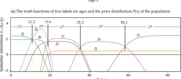
Figure 2 illustrates the relationship between P(x|θj) and T(θj|x) for a given P(x), where x is an

age, the label yj = “Youth”, and θj is a non-fuzzy set and, hence, becomes Aj.

Figure 2. Relationship between T(Aj|x) and P(x|Aj) for given P(x).

We use Global Positioning System (GPS) data as an example to demonstrate a semantic Bayes prediction.

Example 1. A GPS device is used in a train, and hence P(x) is uniformly distributed on a line (see Figure 3). The GPS pointer has a deviation. Try to find the most probable position of the GPS device.

Figure 3. Illustrating the positioning of a GPS device with deviation. The round point is the pointed position with a deviation, and the position with the star is the most probable position.

The semantic meaning of the GPS pointer can be expressed by

T(θj|x) = exp[− (x − xj)2/(2σ2)], (15)

where xj isthe pointed position by yj and σ is the Root Mean Square (RMS). For simplicity, we

assume that x is one-dimensional.

According to Equation (13), we can predict that the position indicated by the star in Figure 3 is the most probable position. Most people would make the same prediction without using any mathematical formula. It seems that human brains must automatically use a similar method: making predictions according to the fuzzy denotation of yj.

In semantic communication, we often see hypotheses or predictions, such as “the temperature is about 10 ˚C”, ”the time is about seven o’clock”, or “the stock index will go up about 10% next

month”. Each one of these may be represented by yj= “X is about xj”. We can also express their

truth functions by Equation (15).

The author defines the (amount of) semantic information that is conveyed by yjabout xi with the

log-normalized-likelihood: ( | ) ( | ) ( ; ) log = log . ( ) ( ) i j j i i j i j P x T x I x P x T

θ

θ

θ

θ

Introducing Equation (15) into this formula, we have

2 2

( ; ) log[1/ ( )] (_{i j j i j}) / (2 ),

I x

θ

θ

σ

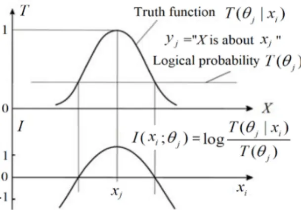
by which we can explain that this information is equal to the Carnap–Bar-Hillel information minus the squared relative deviation. Figure 4 illustrates this formula.

Figure 4. The semantic information conveyed by yj about xi.

Figure 4 indicates that, the smaller the logical probability, the more information there is; and, the larger the deviation is, the less information there is. Thus, a wrong hypothesis will convey negative information. These conclusions accord with Popper’s thought (see [32], p. 294).

To average I(xi; θj), we have generalized KL information

( | ) ( | ) ( ; ) ( | ) log = ( | ) log . ( ) ( ) i j j i j i j i j i i i j P x T x I X P x y P x y P x T

θ

θ

θ

θ





In Equation (18), P(xi|yj) (i = 1,2…) is the sampling distribution, which may be unsmooth or

discontinuous.

Theil proposed a generalized KL formula with three probability distributions [37]. However, in Equation (18), T(θj) is constant. If T(θj|x) is an exponential function with e as the base, and then

Equation (18) will become the Donsker–Varadhan representation [19,38].

Akaike [4] proved that the Least KL divergence criterion is equivalent to the Maximum likelihood (ML) criterion. Following Akaike, we can prove that the Maximum Semantic Information (MSI) criterion (e.g., the maximum generalized KL information criterion) is also equivalent to the ML criterion.

Definition 3. D is a sample with labels {(x(t), y(t))|t = 1 to N; x(t)∈U; y(t)∈V}, which includes n different sub-samples or conditional samples Xj, j = 1,2,…,n. Every sub-sample includes data points x(1), x(2),

…, x(Nj)∈U with label yj. If Xjis large enough, we can obtain the distribution P(x|yj) from Xj. If yj in Xj is

unknown, we replace Xj with X andP(x|yj) with P(x|.).

Assume that there are Njdata points in Xj, where the Nji data points are xi. When Nj data points

in Xj come from Independent and Identically Distributed (IID) random variables, we have the

log (

|

)= log ( (1), (2),..., ( )| ) log

( |

)

( |

) log ( | )= -

( |

).

P

P x

x

x N

P x

N

P x y

P x

N H X

θ

θ

θ

θ

θ

=

=

∏



X

( | )

( ; )

( |

) log

( | )

( |

) log ( )

( )

P x

I X

P x y

H X

P x y

P x

P x

θ

θ

=



= −

θ

+



I(X; θj) and logP(Xj|θj) reach their maxima at the same time that θj changes and, hence, the two

criteria are equivalent. It is easy to prove that, when P(x|θj) = P(x|yj), I(X;θj), and logP(Xj|θj) reach

their maxima.

When the sample Xj is very large, letting P(x|θj) = P(x|yj), we can obtain the optimized truth

function:

T*(θj|x) = [P*(x|θj)/P(x)]/max[P*(x|θj)/P(x)] = [P(x|yj)/P(x)]/max[P(x|yj)/P(x)]. (21)

We can also obtain

T*(θj|x) = P*(θj|x)/max[P*(θj|x)] = P(yj|x)/max[P(yj|x)]. (22)

This formula clearly indicates how the semantic channel matches the Shannon channel, which indicates the use rule of Y. It is also compatible with Wittgenstein's thought: meaning lies in uses (see [39], p. 80).

To average I(X; θj) for different y, we use the Semantic Mutual Information (SMI) formula

( | ) ( | ) ( ; ) ( ) ( | )log = ( ) ( | )log . ( ) ( ) i j j i j i j i j i j i i i j j P x T x I X P y P x y P x P y x P x T

θ

θ

θ

θ







If P(x|θj) = P(x|yj) or T(θj|x)∝P(yj|x) for different yj, the SMI will be equal to the Shannon Mutual

Information (SHMI).

Introducing Equation (15) into the above formula, we have

2 2 ( ; ) ( ) ( | ) = ( _j) log ( )_j ( ,_{i j})( _{i j}) / (2 _j ). j j i I X H H X P y T P x y x x

θ

θ

θ

θ

σ



 

It is clear that the maximum SMI criterion is a special Regularized Least Squares (RLS) criterion [33]. H(θ) is the regularization term and H(θ|X) is the relative error term. However, H(θ) only penalizes the deviations without penalizing the means. The importance of this is that the maximum SMI criterion is also compatible with the ML criterion.

2.1.2. From the Rate-Distortion Function R(D) to the Rate-Verisimilitude Function R(G)

The function R(G) will be used to explain the convergence of the CM algorithms for the MMI classification and mixture models.

Shannon proposed the rate-distortion function R(D) [30]. R(G) [25] is a new version of R(D). In

R(D), R is the information rate and D is the upper limit of average distortion. R(D) means that, for given D, R(D) is the minimum of SHMI I(X;Y).

The rate distortion function with parameter s (see [48], p. 32) includes two formulae:

( ) ( ) ( ) exp( ) / ( ) ( ) ( ) ln ij i j ij i i j i i i D s d P x P y sd R s sD s P x

λ

λ





where i ( ) exp(j ij)

j

P y sd

λ



Let dij be replaced with Iij= I(xi;θj) = log[T(θj|xi)/T(θj)] = log[P(xi|θj)/P(xi)] and G be the lower

limit of I(X; θ). The information rate for given G and source P(X) is defined as

( | ): ( ; )

( )

min

( ; )

R G

I X Y

=

Popper [32] proposed using verisimilitude, instead of correctness, to evaluate a hypothesis. Verisimilitude includes both correctness and precision. Hence, I(xi;θj) can be a good measure for the

verisimilitude of yj reflecting xi; therefore, we call R(G) the rate-verisimilitude function.

Following the derivation of R(D) ([48], p. 31), we obtain

( ) ( ) ( )2 ) / = ( ) ( ) / ( ) ( ) ( ) log ( | ) / ( ), ( ) ij sI s ij i j i ij i j ij i i j i j i i i s ij j i j i j ij j G s I P x P y I P x P y m R s sG s P x m T x T P y m

λ

λ

λ

θ

θ

λ









where mij= T(θj|xi)/T(θj) = P(xi|θj)/P(xi) is the normalized likelihood and λi = ∑jP(yj)mijs. The shape of

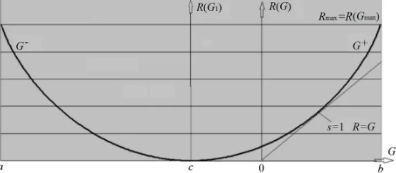
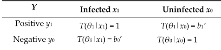
any R(G) function is a bowl-like curve with second derivative > 0, as shown in Figure 5.

Figure 5. The rate-verisimilitude functionR(G) for binary communication. For any R(G) function, there is a point where R(G)=G.

In Figure 5, s= dR/dD. When s = 1, R is equal to G, which means that the semantic channel matches the Shannon channel. G/R indicates the efficiency of semantic communication. In Section 3.4, we will see that solving a mixture model is equivalent to finding a parameter set θ that maximizes G/R, such that G/R is close to 1 or G≈R.

When s→∞, R and G both reach their maxima Rmax and Gmax. As s increases, the TPFs P(yj|x), j =

1, 2, …, n, will become steeper and the Shannon channel will have less noise. Hence, R and G will increase. This property of R(G) can be used to prove the convergence of the CM iteration algorithm for the MMI classification of unseen instances.

The function R(G) is different from R(D). For a given R, there exists a maximum value G+ _{and a} minimum value G-; G- is negative, which means that we also need certain objective information R to bring a certain information loss |G| to enemies. When R = 0, G is negative, which means that if we listen to someone who randomly predicts, the information that we already have will be reduced.

The function R(G) was mainly developed for image compression, according to visual discrimination [25]. However, it can also be used for convergence proofs of MMI classification and mixture models.

2.2.FromTraditionalBayesPredictiontoLogicalBayesianInference

To understand LBI better, we will first review Traditional Bayes Prediction (TBP), LI, and BI. Note that “Bayes prediction” means the prediction according to Bayes’ theorem, which is different from “Bayesian prediction” [3] that was made by Bayesians.

We call probability prediction with the TPF P(yj|x) TBP. For given P(x) and P(yj|x), we can

make a probability prediction

P(x|yj) = P(x) P(yj|x)/P(yj). (28)

When P(yj|x) is replaced with kP(yj|x), where k is a constant, P(x|yj) is the same, because

( ) ( | ) ( ) ( | ) = ( | ). ( ) ( | ) ( ) ( | ) j j j i j i i j i i i P x kP y x P x P y x P x y P x kP y x = P x P y x





Using this formula, we can easily explain that a truth function that is proportional to a TPF can be used for the same probability prediction.

For given P(yj), P(x|yj), and P(x), we can obtain the predictive model

P(yj|x) = P(yj) P(x|yj)/P(x). (30)

After P(x) is changed, we can still use P(yj|x) to make a new probability prediction, in most cases

where the Shannon channels are stable.

We use the medical test (or signal detection) as an example to explain how a TPF or a Shannon channel can be used as a predictive model.

Definition 4. Let z be an observed feature for an unseen instance (see Figure 1) and Z be a random variable, taking a value z∈C = {z1, z2, …}. For unseen instance classification, x denotes a true class or true label.

Assume that we classify every unseen instance with an unseen true label x, according to its observed feature z∈C. That is, we provide a classifier y=f(z) to obtain a label y for z (see Figure 6).

Figure 6. Illustrating the medical test and signal detection. We choose yj according to z∈Cj. {C0, C1} is a partition of C.

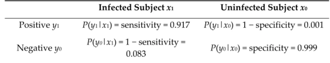
We use the HIV test to explain that the TPF can be used for probability prediction, with different P(x). For an infected subject x1, the conditional probability P(y1|x1) of y1 = positive is called sensitivity, which means the true positive rate. For an uninfected subject x0, the conditional probability P(y0|x0) of y0 = negative is called specificity, which means the true negative rate [49]. The sensitivity and specificity ascertain a Shannon channel, as shown in Table 1.

Table 1. The sensitivity and Specificity of a Medical Test ascertain a Shannon Channel P(Y|X).

Infected Subject x1 Uninfected Subject x0

Positive y1 P(y1|x1) = sensitivity = 0.917 P(y1|x0) = 1 − specificity = 0.001 Negative y0 P(y0|x1) = 1 − sensitivity =

0.083 P(y0|x0) = specificity = 0.999 * Data are obtained from OREQuick HIV tests [50].

Example 2. Calculate P(x1|y1) using P(y1|x) in Table 1 for P(x1) = 0.0001, 0.002 (for normal people),

and 0.1 (for high-risk crowd).

Solution.Using Equation (28), for P(x1) = 0.0001, 0.002, and 0.1, we have P(x1|y1) = 0.084, 0.65, and

0.99, respectively.

While using LI, it is not easy to solve Example 2. Nevertheless, when x is one of many different values and the sample size is not large enough, the TPFs cannot be smooth and, hence, we cannot use a TPF to obtain a smooth P(x|yj). This is why we use LI, which uses parameters to construct

smooth likelihood functions. Using Maximum Likelihood Estimation (MLE), we can use a sample X

to train a likelihood function to obtain the best θj:

*= arg max ( | ) arg max[

( | .) log ( | )],

j j j j i i j i

P

P x

P x

θ

X

θ

=



θ

where P(xi|.) indicates that yj is unknown. The main defect of LI is that LI cannot make use of prior

knowledge and that the optimized likelihood function will be invalid when P(x) is changed. Subjective Bayesians developed Bayesian Inference (BI) to make use of prior knowledge [2,3]. They brought the prior distribution P(θ) of θ into Bayes’ Theorem to obtain the Bayesian posterior

( ) ( | )

( | )

( )=

( ) ( | )

( )

P

P

P

P

P

P

P

θ

θ

θ

X

=

X

X



θ

X

θ

X

，

，

where Pθ(X) is the normalized constant related to θ and P(θ|X) is the posterior distribution of θ or

the Bayesian posterior. Using P(θ|X), we can derive the Maximum A Posterior estimation:

*= arg max ( | ) arg max ( ) ( | )

= arg max[ ( | .) log ( | ) log ( )]

j j j j j j j j i i j j i P P P P x P x P θ θ θ

θ

θ

θ

θ

θ

θ



BI has some advantages, such as

• it is especially suitable to cases where Y is a random variable for a frequency generator, such as a dice;

• as the sample size increases, the distribution P(θ|X) will gradually shrink to some θj* coming

from the MLE; and,

• BI can make use of prior knowledge better than LI. However, BI also has some disadvantages:

• the probability prediction from BI [3] is not compatible with traditional Bayes prediction;

• P(θ) is subjectively selected; and,

• BI cannot make use of the prior of X.

If we try to use BI to solve Examples 1 and 2, we will find that the Bayesian posterior is not as good as TPF P(yj|x). Therefore, to make use of the prior of X, we still want a parameterized TPF P(θj|x).

2.2.2. From Fisher’s Inverse Probability Function P(θj|x) to Logical Bayesian Inference (LBI) De Morgan first called TPF P(yj|x) the “inverse probability”, with respect to Laplace’s method

of probability [2]. The corresponding direct probability is P(x|yj). Later, Fisher called the likelihood

function P(x|θj) the direct probability and the parameterized TPF P(θj|x) the inverse probability [2].

We use θj (instead of θ) and x (instead of xi) to emphasize that θj is a constant and x is a variable,

and hence P(θj|x) should be a function. In the following, we call P(θj|x) the Inverse Probability

Function (IPF). According to Bayes’ theorem,

P(θj|x ) = P(θj) P(x|θj)/P(x), (34)

P(x|θj) = P(xi) P(θj|x)/P(θj). (35)

The IPF P(θj|x) can make use of the prior knowledge P(x) well. When P(x) is changed into P’(x),

we can still obtain P’(x|θj) from P’(x) and P(θj|x).

When n = 2, we can easily construct P(θj|x), j=1,2, with parameters. For instance, we can use a

pair of Logistic (or Sigmoid) functions as the IPFs. Unfortunately, when n > 2, it is hard to construct

P(θj|x), j=1,2,…,n, because there is a normalization limitation ∑jP(θj|x) = 1 for every x. This is why a

multiclass or multilabel classification is often converted into several binary classifications [51,52]. It seems that we may use the Softmax function as the IPF P(θj|x) for n > 2. However, this

function is not compatible with P(yj|x), especially when two or more classes are not exclusive, the

Softmax function does not work.

Using P(θj|x) and P(yj|x) as predictive models also has another disadvantage: In many cases,

we can only know P(x) and P(x|yj) without knowing P(θj) or P(yj), such that we cannot obtain

P(yj|x) or P(θj|x). Nevertheless, we can obtain a truth function T(θj|x) in these cases. In LBI, there is

no normalization limitation and, hence, it is easy to construct a group of truth functions and train them with P(x) and P(x|yj), j=1,2,…,n, without P(yj) or P(θj). This is an important reason why we use

LBI.

When a sample Xj is very large, we can directly obtain T*(θj|x) from Equation (21). For a

size-limited sample, we can use the generalized KL information formula to obtain

( | ) ( | )

( | )

( | ) *( | ) arg max ( ; )= arg max ( | ) log

( ) ( | )

= arg max ( | ) log .

( ) j j j j i j j i j T x T x _{i j} i j i j T x i i T x T x I X P x y T P x P x y P x θ θ θ

θ

θ

θ

θ

θ





This formula is the main formula that is used in LBI. LBI provides the Maximum Semantic Information Estimation (MSIE):

*= arg max ( ; )= arg max[

( | .) log[ ( | ) / ( )]

= arg max[

( | .) log ( | ) log ( )]

j j j j j i i j i i i j i j i

I X

P x

P x

P x

P x

T

x

T

θ

θ

θ

θ

−

θ





，

which is compatible with MLE. If the samples are large enough, the MSIE, MLE, and MAP are equivalent.

We suggest using the truth function as the predictive model or the inferential tool for LBI in some cases, as it has the following advantages:

• we can use an optimized truth function T*(θj|x) to make probability predictions for different

P(x) just as we would use P(yj|x) or P(θj|x);

• we can train a truth function with parameters by a sample with small size, as we would train a likelihood function;

• the truth function indicates the semantic meaning of a hypothesis and, hence, is easy for us to understand;

• it is also the membership function, which indicates the denotation of a label or the range of a class and, hence, is suitable for classification;

• to train a truth function, we only need P(x) and P(x|yj), without needing P(yj) or P(θj); and, • letting T(θj|x)∝P(yj|x), we construct a bridge between statistics and logic.

The CM algorithms further reveal these advantages.

3. Methods II: The Channel Matching (CM) Algorithms 3.1.CM1:ToResolvetheMultilabel-Learning-for-New-P(x)Problem

3.1.1. Optimizing Truth Functions or Membership Functions

We use CM1 to denote the basic matching algorithm, in which the semantic channel matches the Shannon channel, and membership functions or truth functions are used as learning functions.

Assume that x is an age, yjis a label “Youth”, and θj is a fuzzy set {x|x is a youth}. From

population statistics, we can obtain a population age distribution P(x) and a posterior distribution

P(x|yj).

We can directly use Equation (21) to obtain the optimized membership function T*(θj|x)

without parameters if the sample is very large and, hence, the distributions P(x) and P(x|yj) are

smooth. If P(x) and P(x|yj) are not smooth, we can use Equation (36) to obtain T*(θj|x) with

parameters. Without needing P(yj), in CM1, every label’s learning for T*(θj|x) is independent.

If the given sampling distribution is a TPF P(yj|x), we may assume that P(x) is flat.

Subsequently, Equation (36) becomes

( | )

( | ) ( | )

* ( | ) arg max log .

( | ) ( | ) j j i j i j T x _{i j k j k} k k P y x T x T x P y x T x θ

θ

θ

θ

 



If P(yj|x) is smooth, we can use Equation (22) to obtain T*(θj|x) without parameters. For

multilabel learning, we can directly obtain a group of truth functions from a Shannon channel

P(Y|X) or a sample with distribution P(x,y). However, while using popular multilabel learning methods, such as Binary Relevance, we have to prepare several samples for several Logistic functions.

When P(x) is changed, T*(θj|x) is still useful for making semantic Bayes predictions.

3.1.2. For the Confirmation Measure of Major Premises

We use “degree of confirmation” to denote “degree of belief” supported by evidence or samples.

Bayesians use “degree of belief” to explain the subjective probability of a hypothesis. This degree of belief is between 0 and 1. However, researchers of induction use “degree of belief” to evaluate if–then statements or major premises. This degree of belief should be between −1 and 1. In this paper, we take “degree of belief” between −1 and 1 for the subjective evaluation of if–then statements. We know that the correlation coefficient between the two random variables is also between −1 and 1. The difference is that if–then statements are asymmetric; there is more than one major premise and degree of belief between the instance X and the hypothesis Y.

Now, we take the medical test as an example to explain how to use truth functions to replace TPFs or how to use the semantic channel to replace the Shannon channel for probability predictions.

From the Shannon channel in Table 1, we can derive the semantic channel, as shown in Table 2. Assume that T(y1|x1) = T(y0|x0) = 1 and T(y1|x0) = T(y0|x1) = 0 for non-fuzzy hypotheses. Two truth functions for corresponding fuzzy hypotheses are

T(θ1|x) = b1’ +b1T(y1|x), (39) T(θ0|x) = b0’ +b0T(y1|x), (40) where b1 = b(y1→x1), which is the degree of belief of major premise MP1 = y1→x1 = “if Y = y1 then X= x1”,and b1 ’ = 1 − |b1| means the degree of disbelief of MP1 and the ratio of a tautology in y1. Likewise, b0 = b(y0→x0) and b0’ = 1 − b0.

Table 2. The two degrees of disbelief of the medical test form a semantic channel T(θ|X).

Y Infected x1 Uninfected x0

Positive y1 _{T(θ1|x1) = 1 T(θ1|x0) =b1’} Negative y0 T(θ0|x1) = b0’ T(θ0|x0) = 1

According to Equations (21) and (22), the two optimized degrees of disbelief are

b1’*=P(y1|x0)/ P(y1|x1) = [P(x0|y1)/P(x0)]/[P(x1|y1)/P(x1)], (41) b0’*=P(y0|x1)/P(y0|x0) = [P(x1|y0)/P(x1)]/[P(x0|y0)/P(x0)]. (42) For given y1, we can use b1’* and different P(x) to make the semantic Bayes prediction:

P(x1|θ1) = P(x1)/[P(x1) + b1’*P(x0)], (43) P(x0|θ1) = b1’*P(x0) /[P(x1) + b1 ’*P(x0)]. (44) This prediction is equivalent to the traditional Bayes prediction with the TPF P(yj|x). We can still

make the prediction, even if we only know P(x|y1) and P(x) without knowing P(y1). It is easy to verify that, while using Equation (43) to solve Example 2, the results are the same as those that were obtained from the traditional Bayes prediction.

We will find it is not easy for the model to fit different P(x) if we try to use LI or BI to obtain a predictive model for medical tests.

In comparison with the Shannon channel in Table 1, the semantic channel in Table 2 is easier to understand and remember. To remember P(y1|x), we need to remember two numbers; whereas, to remember T*(θ1 |x), we only need to remember one number b1’*.

In [41], the author provided two formulae for positive and negative degrees of confirmation. These two formulae can be merged into a new formula:

1 1 1 0

1 1 1

1 1 1 0

( | ) ( | ) sensitivity-(1-specificity)

* *( )

max( ( | ), ( | )) max(sensitivity 1-specificity) True_ positive_ rate False_positive_rate

max(True_ positive_ rate, False_positive_rate)

P y x P y x b b y x P y x P y x C − = → = = − = = ， 1 1 1 1 ' max( , ') L CL CL CL − _， (45)

where CL1 = P(y1|x1)/[P(y1 |x0) + P(y1 |x1 )] is the confidence level of MP1 and CL1 ’ = 1 − CL1 . As CL1 changes from 0 to 1, b1* changes from −1 to 1, as shown in Figure 7.

Figure 7. Relationship between degree of conformation b* and confidence level CL. As CL changes from 0 to 1, b* changes from −1 to 1.

3.1.3. Rectifying the Parameters of a GPS Device

If we do not know the real parameters of a GPS device or are suspicious of the parameters claimed by the producer, we can assume

T(θj|x) = exp[− |x − (xj+△x)|2/(2σ2)], (46)

where x is a two-dimensional vector. Subsequently, we can use a sample to find the parameters △x

(the systematic deviation) and σ. We may obtain the sample by driving a car with the GPS device around a big square and recording the relative positions x’ = x−xj. From many relative deviations,

we can obtain a sampling distribution P(x’|yj). As we are driving on a big square, P(x) should be

flat. Afterwards, we can use the generalized KL information formula to obtain the optimized parameters △x* and σ*. Subsequently, we replace yj with yk= ”X is about xk”, where xk=xj+△x*.

Assuming that the GPS device is often faulty, we can also use

T(θj|x) = b exp[−|x− (xj + △x)|2/(2σ2)] + 1 − b (47)

as the learning function to obtain the degree of confirmation b* of the GPS device.

If one tries to use the inverse likelihood function P(θj|x) or the Bayesian posterior P(θ|X) for

the above task and probability prediction (see Figure 3), they will find that it is difficult to do, because they only have prior knowledge P(x) from a GPS map, without prior knowledge P(y) or

P(θ).

3.2.CM2:TheSemanticChannelandtheShannonChannelMutuallyMatchforMultilabelClassifications

CM2 includes two steps：

• Matching I: Let the semantic channel match the Shannon channel or use CM1 for multilabel learning; and,

• Matching II: Let the Shannon channel match the semantic channel by using the Maximum Semantic Information (MSI) classifier.

Both steps use the MMI or ML criterion.

For multilabel learning, we may train every label by Equation (36) or Equation (38). We may also train a label yj with membership function T(θj|x) and its negative label yj’ with membership

function 1 − T(θj|x), at the same time, as in the popular method of [51,52], by

( | )

( | )

*( | ) arg max[ ( ; ) ( ; )]

( | ) 1 ( | )

= arg max [ ( | )log ( | )log ]

( ) 1 ( ) j j c j j j T X j i j i i j i j T x _{i j j} T x I X I X T x T x P x y P x y T T θ θ

θ

θ

θ

θ

θ

θ

θ



where θjc is the complementary set of θj. The obtained T*(θj|x) may be a Logistic function, which

will cover a larger area of U, in comparison with T*(θj|x) from Equation (36) or Equation (38).

If there are examples with one instance and several labels, or with several instances and one label, we may split such an example into several single-instance and single-label examples, in the manner of the popular method in [51]. Subsequently, we can obtain the Shannon channel P(Y|X) for multilabel learning.

For classifications where instances are visible, x is given. In Matching II, the MSI classifier is *= ( ) arg max log ( ; )= arg max log[ ( | ) / ( )]

j j

j j j j

y y

y h x = I x

θ

θ

θ

While using T(θj), we can overcome the class-imbalance problem [50] and reduce the rate of

becomes Carnap and Bar-Hillel’s semantic information measure, and the classifier becomes the minimum logical probability classifier:

with ( | ) 1 with ( | ) 1

*= ( ) arg max log[1 / ( )]= arg min log ( )

j j j j j j j y T A x y T A x y h x T A T

θ

This criterion encourages us to select a compound label with smaller denotation.

For unseen instance classifications or uncertain x, we only have knowledge of P(x|z). Afterwards, the MSI classifier becomes

( | )

*

( ) arg max

( | )log

.

( )

T

x

y

f z

P x z

T

θ

θ

=

=



To simplify multilabel learning, we may train fewer atomic labels and use them and the fuzzy logic, which is compatible with Boolean algebra [22] to produce the membership function of a compound label for multilabel classifications [44].

In the popular method for multilabel classifications while using the Bayes classifier or the MPP criterion, for different x the classifier compares two IPFs P(θj|x) and P(θk|x), such as two Logistic

functions, to select a label with greater IPF. This method is not compatible with the information criterion or the likelihood criterion.

3.3.CM3:theCMIterationAlgorithmforMMIclassificationofUnseeninstances

We use CM3 to denote the CM iteration algorithm, which repeats the two matching steps (i.e., Matching I and Matching II). CM2 is not an iterative algorithm; nevertheless, CM3 is. This algorithm is used for MMI classification, for which the most popular method is Gradient Decent.

We use the medical test, as shown in Figure 6, as an example to explain the problem with the MMI classification of unseen instances.

We need to optimize z’ for the MMI. The problem is that, without the classifier f(z), we cannot express the mutual information I(X; Y); whereas, without the expression of mutual information, we cannot optimize the classifier f(z). This problem is also met by MLE for uncertain Shannon channels. To resolve this problem, researchers generally use parameters to construct partition boundaries and then use Gradient Descent or the Newton method to search for the best MMI parameters. The CM iteration algorithm for MMI classification is different. It uses numerical values to express boundaries and information gain functions (e.g., reward functions). It repeatedly updates information gain functions and boundaries to achieve MMI.

Let Cj be a subset of C and yj= f(z|z∈Cj); hence, S = {C1, C2, …} is a partition of C. Our aim is, for given P(x,z) from D, to find the optimized S, as given by

( | )

* arg max ( ; | ) arg max ( ) ( | ) log

( ) j i j i j S S _{j i j} T x S I X S P C P x C T

θ

θ

θ



Matching I: Let the semantic channel match the Shannon channel. First, we obtain the Shannon channel for a given S:

(

| )

( | ),

1, 2,...,

P y x

P z x j

n

=



=

From this Shannon channel, we obtain the semantic channel T(θ|X) and the semantic information I(xi; θj). Subsequently, for given z, we obtain the information gain functions:

( ; | )_{i j} ( | ) ( ; )_{i i j}

i

I X

θ



θ

(54)

which are some curved surfaces over a two-dimensional feature space, as U is two-dimensional. We may directly let I(xi; θj) = I(xi; yj) = log[P(yj|x)/P(yj)]. However, with the notion of the semantic

Matching II: Let the Shannon channel match the semantic channel by the classifier * ( ) arg max ( ; | ) j j i j y y =f z = I X

θ

Repeat Matching I and II until S does not change. The convergent S is the S* we seek.

Using Matching II for the optimization of the Shannon channel can reduce noise. We can understand the two matching steps in this way: Matching I is for the reward function; Matching II is for the Bayes decision.

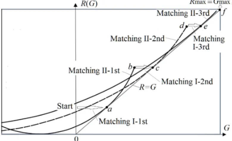
For a given source P(X), a semantic channel ascertains an R(G) function. An improved R(G) function has a higher matching point; that is, where R(G) = G. CM3 finds this matching point, which is also the point that attains Rmax and Gmax (see Figure 8).

Figure 8. Illustrating the iterative convergence of the MMI classification of unseen instances. In the iterative process, (G,R) moves from the start point to a,b,c,d,e,…,f gradually.

We can prove that the iteration will converge. In the iterative process, the coordinate (G,R) changes, as follows:

Matching I-1st Matching II-1st Matching I-2nd Matching II-2nd Matching I-3rd Matching II-3rd

Start

...

a

b

c

d

e

f

⎯⎯⎯⎯⎯

→ ⎯⎯⎯⎯⎯→ ⎯⎯⎯⎯⎯→ ⎯⎯⎯⎯⎯→

⎯⎯⎯⎯⎯

→ ⎯⎯⎯⎯⎯→

This process continues until Matching II cannot improve R and G.

The coordinate (G,R) can converge to (Gmax, Rmax), as every Matching I procedure increases G

and every Matching II procedure increases G and R, and the maxima of G and R are finite.

Matching II can always find any best partition for given I(X;yj|z), j=1,2,…, because it checks

every z to see which of the I(X;yj|z), j=1,2…, is the maximum.

We can understand the CM iteration algorithm in the following way: The function R(G) is like a ladder, and the coordinate (G,R) is like a climber. In Matching I, (G,R) creates a ladder and then moves on it. In Matching II, it climbs up to the top of the ladder. Afterwards, the process is repeated, creating new ladders until (Gmax, Rmax) is reached.

3.4.CM4:theCM-EMAlgorithmforMixtureModels

We use CM4 to denote the CM-EM Algorithm: An Improved Expectation-Maximization (EM) Algorithm for mixture models.

In CM3, Matching II is used to find the maximum R, whereas, in CM4, Matching II is used to find the maximum information efficiency G/R or minimum R−G.

CM4 is based on a different convergence theory of the mixture models. The popular convergence theory of the EM algorithm explains that we can maximize the incomplete data log-likelihood LX(θ) by maximizing the complete data log-likelihood Q, whereas the convergence

theory of the CM-EM algorithm explains that we can maximize LX(θ) by maximizing the information

efficiency G/R.

The EM algorithm [53] for mixture models has been shown to often result in slow or invalid convergence [54,55]. We can improve the EM algorithm by letting the semantic channel and the Shannon channel mutually match. The difference is that Matching II is used to find the minimum of the Shannon mutual information R.

If a probability distribution Pθ(x) comes from the mixture of n likelihood functions, such as

1 ( ) ( ) ( | ) n j j j P x_θ P y P x θ = =



Subsequently, we call Pθ(x) a mixture model. If every predictive model P(x|θj) is a Gaussian

function, then Pθ(x) is a Gaussian mixture. In the following, we use n = 2 to discuss the algorithms

for mixture models.

Assume that P(x) comes from the mixture of two true model P(x|θ1 *) and P(x|θ2*) with ratios of P*(y1) and P*(y2) = 1 − P*(y1); that is,

P(x)=P*(y1)P(x|θ1*)+P*(y2)P(x|θ2*). (57) We only know P(x) and n = 2. We can use the guessed parameters and mixture ratios to obtain

Pθ(x) = P(y1)P(x|θ1) + P(y2)P(x|θ2). (58) Subsequently, we have the observed data log-likelihood

( ) ( ) log ( ) ( ),

X i i

i

L

θ



and the relative entropy or KL divergence:

( )

( ||

)

( ) log

( )

( ).

( )

P x

H P P

P x

H X

H X

P x

=



=

−

If the two distributions P(x) and Pθ(x) are close to each other, such that the relative entropy is

close to 0, for example, less than 0.001 bit for a huge sample or 0.01 bit for a sample with size = 1000, then, we may say that our guess is right. Therefore, our task is to change θ and P(y) to maximize the likelihood LX(θ) = logP(X|θ) or to minimize the relative entropy H(P||Pθ).

The main formula of the EM algorithm for mixture models can be described, as follows:

( ) ( | ) log ( ,

| )

( )

( ) (

| ) log (

| )

Q N

P x P y x

P x y

L

N

P x P y x

P y x

θ

θ

=

=

+





，

where Q= − NH(X,Y|θ) is called the complete data log-likelihood and P(yj|x) is from Equation (63).

There exists

LX(θ) = Q + H, (62)

where H = − NH(Y|X,θ) is a Shannon conditional entropy. A popular convergence theory of the EM algorithm explains that we can increase LX(θ) by increasing Q.

The steps in the EM algorithm are:

E-step: Write the conditional probability functions (e. g., the Shannon channel):

(

| )

( ) ( | ) /

( ),

( )

( ) ( | ).

P y x

P y P x

P x

P x

P y P x

θ

θ

=

=



M-step: Improve P(y) and θ to maximize Q. If Q cannot be further improved, then end the iteration process; otherwise, go to the E-step.

Neal and Hinton [56] proposed an improved EM algorithm, the Maximization–Maximization (MM), in which Q is replaced with F = Q + H(Y) and F is maximized in both steps.

Almost all of the EM algorithm researchers believe that Q and logLX(θ) are positively correlated and that the E-step does not decrease Q; nevertheless, this is not true. The author found that Q may decrease in some E-steps; and, Q and F should decrease in some cases [42].

Using the CM algorithm to improve the EM algorithm, we have developed an algorithm, the CM-EM algorithm, for better convergence.

The CM-EM algorithm includes three steps:

E1-step: Construct the Shannon channel. This step is the same as the E-step of the EM algorithm.

E2-step: Repeat the following three equations until P+1_{(y) converges to P(y):} 1 1

( )

( ) (

| )

( ) (

| ),

1, 2,...;

( )

( );

(

| )

( | ) ( ) /

(

( | ),

1, 2,...;

1, 2,...

P

y

P x P y x

P x P y x

j

P y

P

y

P y x

P x

θ

P y

P y P x

θ

i

j

=

=

=

=

=

=

=







）

If H(P||Pθ) is less than a small value, then end the iteration.

MG-step: Optimize the parameters θj+1 of the likelihood function in log(.) to maximize G：

+1

( | )

( |

)

( ; )=

( )

( ) log

( )

( )

P x

P x

G I X

P x

P y

P x

P x

θ

θ

θ

=



Then, go to the E1-step.

As G reaches a maximum when P(x|θj+1)/P(x) = P(x|θj)/Pθ(x), the new likelihood function is

P(x|θj+1) = P(x)P(x|θj)/Pθ(x). (66)

Without the E2-step, P(x|θj+1) above is, in general, not normalized [57]. For Gaussian mixtures,

we can easily obtain new parameters:

1 1 1 1 2 0.5

( ) ( | ) /

( ),

1, 2,..., ;

{

( )[ ( |

)

] } ,

1, 2..., .

P x P x

P x

j

n

P x P x

j

n

μ

θ

σ

θ<