POUR L'OBTENTION DU GRADE DE DOCTEUR ÈS SCIENCES
acceptée sur proposition du jury: Prof. C. N. Jones, président du jury Dr A. Karimi, Dr M. Martino, directeurs de thèse
Prof. M. Heertjes, rapporteur Prof. S. Formentin, rapporteur
Prof. D. Dujic, rapporteur
Controller Design via Convex Optimization
THÈSE N
O8305 (2018)
ÉCOLE POLYTECHNIQUE FÉDÉRALE DE LAUSANNE
PRÉSENTÉE LE 16 FÉVRIER 2018À LA FACULTÉ DES SCIENCES ET TECHNIQUES DE L'INGÉNIEUR LABORATOIRE D'AUTOMATIQUE 3
PROGRAMME DOCTORAL EN GÉNIE ÉLECTRIQUE
Suisse 2018 PAR
You must be ready to give up even the most attractive ideas when experiment shows them to be wrong. — Alessandro Volta
The writing and completion of this dissertation would not have been possible without the assistance, support, and guidance of the many special people in my life. Firstly, I would like to thank God for giving me the capability to contribute to the engineering world and hopefully assist the future civilizations in creating technologies for the good of mankind. I hope that ethical values will be exercised and that the technologies arising from the new frontiers of science are used in conscientious manners.
Secondly, I would like to thank my EPFL advisor, Dr. Alireza Karimi. I have learned many things from him since starting my Ph.D, and I thank him for accepting me into his program. His contributions and patience were key factors in the successful completion of this dissertation. I would also like to thank my CERN supervisor, Dr. Michele Martino. He has been very helpful during my Ph.D studies, and I have enjoyed the numerous technical discussions I had with him; I always learned something new from each discussion, and am very appreciative for that. Among my other CERN colleagues, I would like to also thank Miguel Cerqueira Bastos, Quentin King, Olivier Michele, Davide Aguglia, Todor Todorvic, Ivan Jovetic, Olivier Founier, and Louis De Mallac. The knowledge that I have acquired from Michele and my numerous colleagues will be something that I will foster and cherish for the rest of my life. Among other EPFL personnel and members of other universities that I have collaborated with, I would like to thank Prof. Colin Jones (president of my jury committee), Prof. Dan Simon, Prof. Dominique Bonvin, Prof. Kiril Streletzky, Prof. Marcel Heertjes, and Prof. Simone Formentin.
In addition to my work colleagues, I would also like to thank Zlatko Emedji and Jose Manuel De Paco Soto for being good friends and providing the emotional support I needed. Also a thank you to Predrag Milosavljevic and Christoph Kammer for being good competitors at Foosball during my time at EPFL. Additionally, I would like to thank Michael Davis, Hugo Lebreton, Miguel Hermo Serans, Mahdieh Sadat Sad Abadi, Ioannis Lymperopoulos, Timm Faulwasser, Philippe Muellhaupt, and all other CERN and EPFL colleagues for our random technical and non-technical discussions. A special thank you to Ruth Benassi for her continued support for all administrative work and Christophe Salzmann for his support on technical related issues in the laboratories.
Finally, I would like to thank my family for their support during this endeavour. To my wife Iuliia for her continued support and love, I thank you for everything you have done and being born into this world. I am utterly grateful to be with you and could not wish for anything else. My sisters Carmen, Marie, and Elizabeth have been great inspirations to me; they shaped me into the person I am today and can honestly say that without them, I may not have been so
successful. To my mother, I thank you for everything you have done for me during my 34 years on this planet. I appreciate all of the hard work that you have done to support the family, and I will always carry your love in my heart. And finally, to my father, I wish you could have still been with us to witness this moment in my life. I know that you would have been proud of me, and am very grateful for all of the sacrifices you made for the family.
The objective of this dissertation is to develop data-driven frequency-domain methods for designing robust controllers through the use of convex optimization algorithms. Many of today’s industrial processes are becoming more complex, and modeling accurate physical models for these plants using first principles may be impossible. Albeit a model may be available; however, such a model may be too complex to consider for an appropriate controller design. With the increased developments in the computing world, large amounts of measured data can be easily collected and stored for processing purposes. Data can also be collected and used in an on-line fashion. Thus it would be very sensible to make full use of this data for controller design, performance evaluation, and stability analysis. The design methods imposed in this work ensure that the dynamics of a system are captured in an experiment and avoids the problem of unmodeled dynamics associated with parametric models. The devised methods consider robust designs for both linear-time-invariant (LTI) single-input-single-output (SISO) systems and certain classes of nonlinear systems.
In this dissertation, a data-driven approach using the frequency response function of a system is proposed for designing robust controllers withH∞performance. Necessary and sufficient conditions are derived for obtainingH∞performance while guaranteeing the closed-loop stability of a system. A convex optimization algorithm is formulated to obtain the controller parameters which ensure system robustness; the controller is robust with respect to the frequency-dependent uncertainties of the frequency response function. For a certain class of nonlinearities, the proposed method can be used to obtain a best-linear-approximation with an associated frequency-dependent uncertainty to guarantee the stability and performance for the underlying linear system that is subject to nonlinear distortions.
The controller for this design scheme is presented as a ratio of two linearly-parameterized transfer functions; in this manner, the numerator and denominator of a controller are simul-taneously optimized. With this construction, it can be shown that as the controller order increases, the solution to the convex problem converges to the global optimal solution of theH∞problem. This method is then extended to the 2-degree-of-freedom discrete-time controller where the necessary and sufficient conditions are imposed for multiple weighted sensitivity functions.
The concepts behind these design methods are then used to devise necessary and sufficient conditions for ensuring the closed-loop stability of systems with sector-bounded nonlineari-ties. The conditions are simple convex feasibility constraints which can be used to stabilize systems with multi-model uncertainty. Additionally, a method is proposed for obtainingH∞
performance for systems with uncertain gains within these sectors.
By convexifying theH∞problem, the global optimal solution to an approximate problem is obtained. For low-order controllers, the solution to this approximate problem may lead to solutions far from the optimal solution of the trueH∞problem. Thus two methods are proposed to address this issue for low-order controllers. In one method, a non-convex problem is formulated which optimizes the basis function parameters of a controller while guaranteeing the stability of the closed-loop systems. In another method, a set of convex problems are solved in an iterative fashion to obtain the desired performance (which also guarantees the closed-loop stability of the system). With both methods, the local solution to theH∞problem for fixed-structure controllers is obtained. However, the convex problem is computationally tractable and can also considerH2performance.
The effectiveness of the proposed method(s) is illustrated by considering several case studies that require robust controllers for achieving the desired performance. The main applicative work in this dissertation is with respect to a power converter control system at the European Organization for Nuclear Research (CERN) (which is used to control the current in a magnet to produce the desired field in controlling particle trajectories in particle accelerators). The proposed design methods are implemented in order to satisfy the challenging performance specifications set by the application while guaranteeing the system stability and robustness using data-driven design strategies.
Key words: Convex optimization, data-driven control, fixed-structure control,H∞control, H2control, nonlinear control, power converter control, robust control, sector nonlinearity.
L’objectif de cette thèse est de développer des méthodes de domaine fréquentiel pilotées par les données pour la conception de contrôleurs robustes grâce à l’utilisation d’algorithmes d’optimisation convexe. De nombreux procédés industriels actuels deviennent de plus en plus complexes et il peut être impossible de modéliser des modèles physiques précis pour ces plantes en utilisant les principes premiers. Bien qu’un modèle puisse être disponible ; cepen-dant, un tel modèle peut être trop complexe à considérer pour une conception de contrôleur appropriée. Avec les développements accrus dans le monde informatique, de grandes quan-tités de données mesurées peuvent être facilement collectées et enregistrées à des fins de traitement. Les données peuvent également être collectées et utilisées en ligne. Il serait donc judicieux de tirer pleinement parti de ces données pour la conception du contrôleur, l’évalua-tion des performances et l’analyse de la stabilité. Les méthodes de concepl’évalua-tion imposées dans ce travail garantissent que la dynamique d’un système est capturée dans une expérience et évite le problème de la dynamique non modélisée associée aux modèles paramétriques. Les méthodes développées prennent en compte des conceptions robustes pour les systèmes à entrée unique à sortie unique (SISO) linéaire invariant de temps (LTI) et pour certaines classes de systèmes non-linéaires.
Dans cette thèse, une approche basée sur les données utilisant la fonction de réponse en fréquence d’un système est proposée pour concevoir des contrôleurs robustes avec des per-formancesH∞. Les conditions nécessaires et suffisantes sont dérivées pour obtenir des performancesH∞tout en garantissant la stabilité en boucle fermée d’un système. Un algo-rithme d’optimisation convexe est implémenté pour obtenir les paramètres du contrôleur qui assurent la robustesse du système ; le contrôleur est robuste par rapport aux incertitudes dépendantes de la fréquence de la fonction de réponse en fréquence. En effet, pour une certaine classe de non-linéarités, la méthode proposée peut être utilisée pour obtenir une meilleure approximation linéaire avec une incertitude dépendante de la fréquence associée pour garantir la stabilité et la performance du système linéaire sous-jacent aux distorsions non-linéaires.
Le contrôleur pour ce schéma de conception est présenté comme un ratio de deux fonctions de transfert paramétrées linéairement ; dans cette manière, le numérateur et le dénominateur d’un contrôleur sont simultanément optimisés. Avec cette construction, on peut montrer qu’à mesure que l’ordre du contrôleur augmente, la solution au problème convexe converge vers la solution optimale globale du problèmeH∞. Cette méthode est ensuite étendue au contrôleur à temps discret à 2 degrés-de-liberté où les conditions nécessaires et suffisantes sont imposées
pour des fonctions de sensibilité pondérées multiples.
Les concepts qui sous-tendent ces méthodes de conception sont ensuite utilisés pour conce-voir les conditions nécessaires et suffisantes pour assurer la stabilité en boucle fermée des systèmes avec des non-linéarités liées au secteur. Les conditions sont de simples contraintes de faisabilité convexes qui peuvent être utilisées pour stabiliser des systèmes avec une incerti-tude multimodèle. De plus, une méthode est proposée pour obtenir des performancesH∞ pour les systèmes dont les gains sont incertains dans ces secteurs.
En convexisant le problèmeH∞, on obtient la solution optimale globale à un problème approximatif. Pour les contrôleurs de bas-ordre, la solution à ce problème approximatif peut conduire à des solutions loin de la solution optimale du vrai problème H∞. Ainsi, deux méthodes sont proposées pour résoudre ce problème pour les contrôleurs de bas-ordre. Dans une méthode, un problème non convexe est formulé qui optimise les paramètres de fonction de base d’un contrôleur tout en garantissant la stabilité des systèmes en boucle fermée. Dans une autre méthode, un ensemble sur des problèmes convexes est résolu de manière itérative pour obtenir la performance désirée (ce qui garantit également la stabilité en boucle fermée du système). Avec les deux méthodes, la solution locale au problèmeH∞pour les contrôleurs de structure fixe est obtenue. Cependant, le problème convexe est informatiquement tractable et peut également considérerH2performance.
L’efficacité de la méthode proposée est illustrée en considérant plusieurs exemples qui néces-sitent des contrôleurs robustes pour atteindre la performance souhaitée. Le principal travail applicatif de cette thèse porte sur un système de contrôle de convertisseur de puissance au CERN (qui est utilisé pour contrôler le courant dans un aimant afin de produire le champ souhaité pour contrôler les trajectoires de particules dans les accélérateurs). Les méthodes de conception proposées sont mises en œuvre afin de satisfaire les spécifications de performance difficiles définies par l’application tout en garantissant la stabilité et la robustesse du système à l’aide de stratégies de conception pilotées par les données.
Mots clefs : Optimisation convexe, contrôle piloté par les données, contrôle à structure fixe, contrôleH∞, contrôleH2, contrôle non-linéaire, contrôle du convertisseur de puissance, contrôle robuste, non-linéarité sectorielle.
1DOF 1-Degree-Of-Freedom 2DOF 2-Degree-Of-Freedom ARE Algebraic Riccati Equations BLA Best Linear Approximation BP Bilinear Programming CbT Correlation-based Tuning
CERN Conseil Européen pour la Recherche Nucléaire (European Organi-zation for Nuclear Research)
CPU Central Processing Unit DF Describing Function
FGC Function Generator Controller FRF Frequency Response Function HJI Hamilton-Jacobi-Isaacs
ICbT Iterative Correlation based Tuning IFT Iterative Feedback Tuning
KYP Kalman-Yakubovich-Popov LMI Linear Matrix Inequality LP Linearly Parameterized LPV Linear Parameter-Varying LQG Linear-Quadratic-Gaussian LTI Linear Time-Invariant MFAC Model-Free Adaptive Control MIMO Multiple-Input-Multiple-Output MPC Model Predictive Control
MRAC Model Reference Adaptive Control MRC Model Reference Control
PI Proportional-Integral
PID Proportional-Integral-Derivative PRBS Pseudorandom Binary Sequence PSO Particle Swarm Optimization RL Resistive(R)-Inductive(L) SDP Semi-Definite Programming
SDRE State-Dependent Riccati Equation SIP Semi-Infinite Programming SISO Single-Input-Single-Output SPR Strictly Positive Real UC Unfalsified Control
List of Operators and Conventions
RH∞ The set of all stable, proper, real-rational transfer func-tions with bounded infinity norms.
ρ Transponse of the vectorρ.
H≺0 Strict matrix inequality of a symmetric matrixH.
ℑ{·} Imaginary part of a complex variable.
C The set of all complex numbers.
R The set of all real numbers.
Rn The set of all real vectors of dimensionn.
Rm×n The set of realm×nmatrices.
R+ The set of all real numbers greater than zero.
Z The set of non-negative integers.
F{·} Fourier transform of the argument.
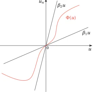
Φ(u) Nonlinear function of an input signalu.
ℜ{·} Real part of a complex variable.
σ2 x y=Q1−1
Q
q=1(x
[q]−x)(y[q]−y)∗ Sample covariance ofQrealizations ofxandy.
σ2 x=Q1−1
Q
q=1|x[q]−x|2 Sample variance ofQrealizations ofx.
A(jω) Frequency response function ofA(s).
A(ejω)/A(e−jω) Frequency response function ofA(z)/A(z−1).
A(s) Transfer function of continuous-time system.
A∗ Complex conjugate of the complex numberA. C(β,rd) Disk associated with Circle criterion (centered atβ
with radiusrd).
f :A→B f is a function on the set of the domain off ⊆Ainto the setB.
|A| =[ℜ{A}]2+[ℑ{A}]2 The magnitude of a complex numberA.
||A||∞=supω|A(jω)| Infinity norm of the complex functionA(jω) (the same operation applies forA(e−jω)) .
||A||p= 1 2π Ωc|A(jω)| pdωp−1 p-norm ofA(jω) forp∈[1, 2, . . . ,∞[ .
List of Symbols
α Uncertain gain within a sector-bounded nonlinearity.
αp The significance level of aχ2distribution.
β Center of the diskC(β,rd).
β1,β2 Slopes of the lines which bound a sector nonlinearity.
φ Vector of stable orthogonal basis functions.
ρ Vector of decision variables.
θp Vector of parameteric uncertainties.
δm Additive disk uncertainty parameter associated with
the coprimeM.
δn Additive disk uncertainty parameter associated with
the coprimeN.
Number of models of a multimodel process.
ι Constriction coefficient of PSO algorithm.
Di Frequency spectrum of a process input disturbance.
Do Frequency spectrum of a process output disturbance.
Nt The set of all sector-bounded time-varying nonlineari-ties.
R Frequency spectrum of the signalr.
Sq qthsensitivity function of a closed-loop system.
Sd
q Desiredqthsensitivity function of a closed-loop
sys-tem. Si
q qthsensitivity function of a closed-loop system with
respect to theithplant model.
U Frequency spectrum of the signalu.
Un Frequency spectrum ofun.
V A class of nonlinear systems (i.e., Wiener systems).
X Frequency spectrum of a signal for identifying the
co-prime factors of a linear system in a nonlinear closed-loop structure.
Y Frequency spectrum of the signaly.
YS Spectrum of error term which is used to describe a
nonlinear system inV.
Ω The set of discrete-time frequencies.
ω Frequency in rad s−1.
Ωc The set of continuous-time frequencies.
σ2
A Variance associated with the measurements of system
A.
θ1,θ2,θ3 Cognitive learning rate, social learning rate, and learn-ing rate, respectively (used in the PSO algorithm). ˜
M Set of additive uncertainty associated with coprime
M. ˜
N Set of additive uncertainty associated with coprimeN.
ϑ PSO penalty factor.
ξ Laguerre parameter for continuous-time controller.
ζd Desired damping factor associated with a second order transfer function.
ζi Poles of a generalized orthonormal basis function.
fd Desired closed-loop bandwidth.
G General representation of a linear plant model.
Gi ithmodel of a multimodel process.
GV A plant model which belongs to the class of systems in
V.
K Controller for 1-degree-of-freedom structure.
L General representation of an open-loop system.
M Coprime factor of a plant modelG.
mp mp sided polygon to approximate the ellipse from a
model’s parameteric uncertainty.
N Coprime factor of a plant modelG.
nr,ns,nt Order of the polynomialsR,S, andT, respectively.
px Number of particles in PSO algorithm.
R Polynomial of discrete-time controller.
r Reference input of a closed-loop system.
rd Radius of the diskC(β,rd).
S Polynomial of discrete-time controller.
s Laplace transform variable.
T Polynomial of discrete-time 2DOFRSTcontroller.
Ts Sampling time of a discrete-time system.
u Input signal of a plant/process.
un Output signal of a sector-bounded nonlinearity.
Wq Weighting filter associated with theqthsensitivity
func-tionSq.
Y Coprime factor of controllerK.
y Output signal of a plant/process.
Acknowledgements i
Abstract (English/Français) iii
Abbreviations vii
Nomenclature ix
List of figures xix
List of tables xxiii
1 Introduction 1
1.1 Motivation . . . 1
1.1.1 Brief History on Automatic Control . . . 1
1.1.2 The Data-Driven Paradigm . . . 2
1.2 State of the Art . . . 3
1.2.1 Data-driven Control . . . 3
1.2.2 Fixed-Structure Controller Design . . . 5
1.2.3 Nonlinear Control . . . 7
1.3 Research Objectives . . . 9
1.3.1 Global Solution ofH∞problem . . . 9
1.3.2 Fixed-Structure Controller Design . . . 10
1.3.3 Contributions . . . 11
1.4 Dissertation Structure . . . 12
2 Preliminaries 15 2.1 Class of models . . . 15
2.1.1 General Plant Representation . . . 15
2.1.2 Coprime Representation . . . 18
2.1.3 Nonlinear Models . . . 20
2.2 Class of controllers . . . 26
2.2.1 Polynomial 1DOF Controller . . . 26
2.2.2 RST 2DOF Controller . . . 27
2.3 Control Performance . . . 28
2.3.1 Sensitivity Functions for 1DOF Structure . . . 29
2.3.2 Sensitivity Functions forRSTStructure . . . 29
2.4 Optimization Problems . . . 30
2.5 Conclusion . . . 32
3 RobustH∞Controller Design 33 3.1 Introduction . . . 33
3.2 Convex parameterization of robust controllers . . . 33
3.2.1 Controller objective . . . 33
3.2.2 Nominal and robust performance . . . 36
3.2.3 Multi-model and frequency-domain polytopic uncertainty . . . 38
3.3 Fixed-order controller design . . . 41
3.3.1 Controller parameterization . . . 41
3.3.2 Convergence to the optimal solution . . . 42
3.3.3 Finite number of constraints . . . 43
3.3.4 Solution by linear programming . . . 44
3.4 Case Studies . . . 44
3.4.1 Case 1: Multi-model uncertainty . . . 44
3.4.2 Case 2: Convergence to optimal performance . . . 46
3.4.3 Case 3: Flexible Transmission System . . . 47
3.5 Conclusion . . . 48
4 Robust RST Controller Design with Applications to Power Converters 51 4.1 Introduction . . . 51
4.2 H∞Performance via Convex Optimization . . . 52
4.2.1 General Design Specifications . . . 52
4.2.2 Robust Design . . . 56
4.2.3 Controller Stability . . . 57
4.2.4 Tracking Specifications . . . 58
4.2.5 Convex Optimization via Semi-Definite Programming . . . 59
4.3 Simulation Examples . . . 60
4.3.1 Case 1: Multi-model uncertainty . . . 60
4.3.2 Case 2: Nonlinear Distortions . . . 61
4.4 Case Study: Power Converter Control . . . 67
4.4.1 Power Converters for Particle Accelerators . . . 67
4.4.2 Experimental Test Setup . . . 68
4.4.3 Control Objective . . . 69
4.4.4 Weighting filter selection . . . 70
4.4.5 Synthesis and Experimental Results . . . 71
4.5 Case Study: Torsional Control . . . 73
4.5.1 Weighting filter selection . . . 75
4.6 Conclusion . . . 77
5 Robust Control of Systems With Sector Nonlinearities 79 5.1 Introduction . . . 79
5.2 The Circle Criterion Revisited . . . 80
5.3 Stabilization via the Circle Criterion . . . 82
5.3.1 Case 1: 0<β1<β2 . . . 82
5.3.2 Case 2:β1<0<β2 . . . 85
5.3.3 Case 3: 0=β1<β2 . . . 87
5.4 A Multi-Model Approach for EnsuringH∞Performance . . . 87
5.4.1 Convex Optimization via Semi-Definite Programming . . . 89
5.5 Case Study . . . 90
5.5.1 Stabilization via the Circle Criterion . . . 92
5.5.2 Stabilization with Performance . . . 93
5.6 Conclusion . . . 96
6 H∞Design for Low-Order Fixed-Structure Controllers 99 6.1 Introduction . . . 99
6.1.1 Robust Performance via Convex Optimization . . . 100
6.2 Optimization Problems For Fixed-Struture Design . . . 101
6.2.1 Bilinear Programming . . . 102
6.2.2 Particle Swarm Optimization . . . 103
6.3 Simulation Examples . . . 105
6.3.1 Case 1: Robust PID Design . . . 106
6.3.2 Case 2: Multi-model Uncertainty . . . 108
6.4 Conclusion . . . 112
7 Model-Reference Control for Particle Accelerator Power Converters 113 7.1 Introduction . . . 113 7.2 Control Performance . . . 114 7.2.1 Convex Approximation . . . 114 7.2.2 H∞Performance . . . 116 7.2.3 H2Performance . . . 116 7.2.4 H1Performance . . . 117 7.3 Stability Analysis . . . 119
7.3.1 Initial Stabilizing Controller . . . 121
7.4 Simulation Examples . . . 122
7.4.1 Case 1: Heat Conductor . . . 123
7.4.2 Case 2: Unstable robot prototype . . . 125
7.5 Case Study: Power Converter Control . . . 127
7.5.1 Controller Design . . . 127
8 Conclusion and Future Outlook 135
8.1 Conclusion . . . 135 8.1.1 Future Outlook . . . 137
A H∞Smith Predictor Design for Time-Delayed MIMO Systems via Convex
Optimiza-tion 139
A.1 Introduction . . . 139 A.2 Problem Formulation . . . 140 A.2.1 Class of models . . . 140 A.2.2 Class of controllers . . . 141 A.2.3 Design specifications . . . 141 A.3 Proposed method . . . 142 A.3.1 Primary controller design . . . 144 A.4 Industrial Case Studies . . . 145 A.4.1 Case 1 - SP with fixed time delays . . . 145 A.4.2 Case 2 - SP with uncertain time delays . . . 146 A.4.3 Case 3 - The Shell control problem . . . 148 A.5 Conclusion . . . 152
Bibliography 153
2.1 Nonlinear sector that is bounded by two lines with slopesβ1andβ2. . . 21 2.2 Representation of a nonlinear system by a linear system for a certain class of
inputs. . . 22 2.3 Procedure for measuring the BLA from the FRF of the nonlinear system.G[q,p]is
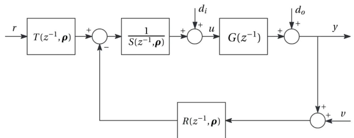
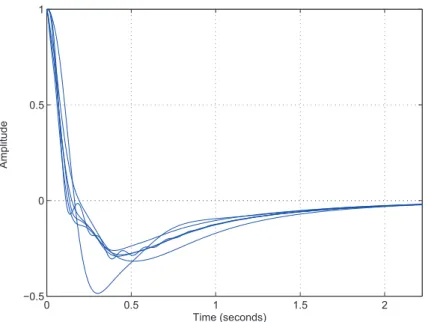
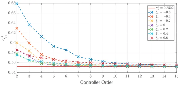
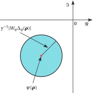
the FRF estimate of thepthperiod of theqthexperiment. . . 23 2.4 Structure to be used in obtaining the coprimes for an unstable process. . . 26 2.5 RST controller structure. . . 27 3.1 Graphical representation of the constraint in 3.1. . . 34 3.2 Illustration of the constraints for polytopic uncertainty with 3 vertices. . . 40 3.3 Step responses for the family of closed-loop systems. . . 46 3.4 γnversus the controller order with different Laguerre parameters. . . 47 3.5 Flexible transmission system . . . 48 3.6 Experimental identification data. . . 49 3.7 Nyquist diagram of the spectral model together with uncertainty disks. . . 49 3.8 Magnitude of the FRF of sensitivity functionSs. . . 50 4.1 The graphical interpretation ofH∞constraints in the complex plane. . . 53 4.2 Optimal solutionγas a function of the controller order. Solutions obtained with
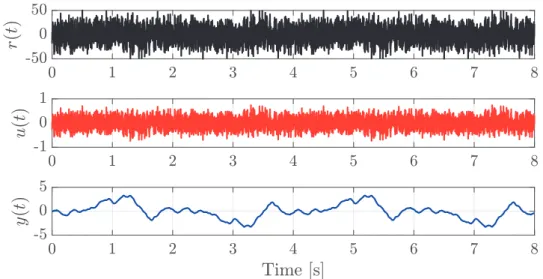
the proposed method (dashed-blue line); solutions obtained with the method which requires the selection of a desired open-loop transfer function (dashed-red line). . . 62 4.3 Random phase multi-sine inputr(t) along with the plant inputu(t) and output
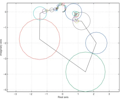
y(t). For presentation purposes, the signals are shown for 2 full periods. . . 63 4.4 N (dashed-blue line) with the associated uncertainties at each frequency (black
circles). The FRF obtained betweenrtoyfor a given experiment with no uncer-tainties (dashed-red line). . . 64 4.5 M(dashed-blue line) with the associated uncertainties at each frequency (black
circles). The FRF obtained betweenr toufor a given experiment with no uncer-tainties (dashed-red line). . . 64 4.6 Variances of coprimes caused by nonlinear distortions . . . 65
4.7 Step response of the nonlinear system. The desired closed-loop response (black line); the response with the proposed method (including uncertainties in design) (blue line); the response with no uncertainties considered (red line). . . 66 4.8 Power converter control system. . . 67 4.9 Fractional dynamics of magnet caused by Eddy currents. . . 68 4.10 The CANCUN used for the control application. . . 69 4.11 The desired reference current profile. The blue-dashed line indicates the time
when the error must remain within±1000 parts-per-million (ppm); the red-dashed line indicates the time when the error must remain within±100 ppm. . 70 4.12 PRBS signal used for the input voltagev(t) of the open-loop system along with
the resulting output currenti(t). . . 71 4.13 Comparison between the error resulting from the model-based design
(solid-black line with red error-bars) and the error resulting with the proposed method (solid-black line with green error-bars). . . 72 4.14 Torsional apparatus (ECP model 205a) used for the experimental analysis. The
three disks are comprised of block masses which can be added or removed to alter the inertia of each disk (and thus alter the dynamics of the system). Each disk is vertically suspended on a spring with a variable spring constant. The actuator is located on the bottom of the device. . . 73 4.15 Time-domain response of the closed-loop system with a PRBS excitation signal
(shown only for the system configuration with two block masses on the top disk): the PRBS reference inputr(t) with a register length of 511 (solid-blue); control outputu(t) (solid-red); output responsey(t) (solid-black). . . 74 4.16 FRF’s of the plant model obtained from the closed-loop time-domain response
of each system configuration. The loads on the bottom and middle disk are fixed while the load on the top disk is varied: FRF with one block mass on the top disk (solid-blue); FRF with two block masses on the top disk (solid-green); FRF with four block masses on the top disk (solid-red). . . 75 4.17 Step response for each load configuration: response with one block mass on
the top disk blue); response with two block masses on the top disk (solid-green); response with four block masses on the top disk (solid-red). . . 77 4.18 Closed-loop frequency response functions of all three system configurations:
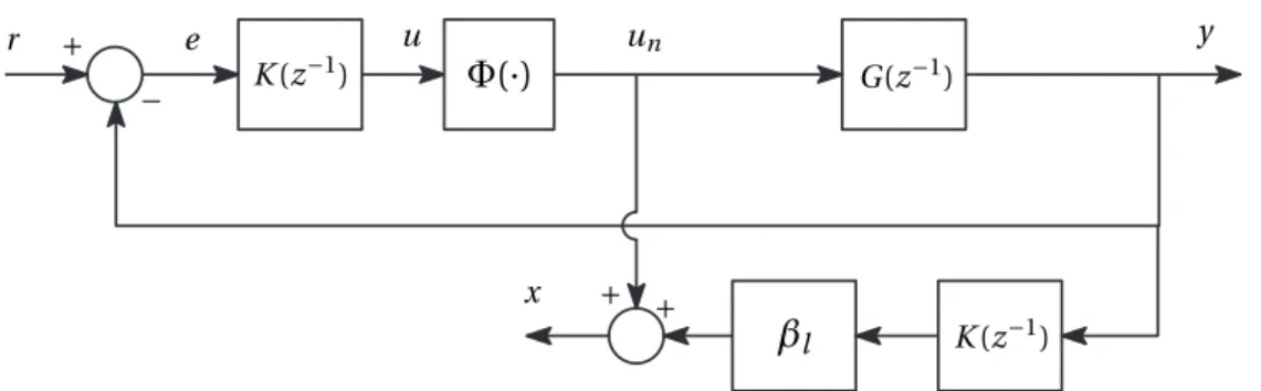
closed-loop FRF with one block mass on the top disk (solid-blue); closed-loop FRF with two block masses on the top disk (solid-green); closed-loop FRF with four block masses on the top disk (solid-red). . . 78 5.1 Discrete-time controller structure. . . 79 5.2 Equivalent block diagram in autonomous form. . . 80 5.3 Absolute stability condition for the sector nonlinearity in (2.14) when different
conditions forβ1andβ2are considered. . . 81 5.4 A graphical interpretation of the constraint (5.5) in the complex plane. . . 83
5.5 Time-varying sector nonlinearity used for the case study. The nonlinearity switches at every positive integer multiple ofTn between the dashed-red line and the solid-red line. . . 91 5.6 Nyquist plot ofLi(e−jω) fori=1, . . . , 4 (solid-blue line); diskC(−2.76, 2.26)
(solid-red line). The Nyquist criterion for the sector-bounded nonlinearity is satisfied for all models. . . 93 5.7 The PRBS signal injected as the reference signalr(t) with the measured responses
forun(t),x(t) andy(t). For illustrative purposes, the figure displays only a small portion of the total signal for the plantG1. . . 94 5.8 Calculated FRFs forN1(solid-blue line),N2(solid-red line),N3(solid-orange
line),N4(solid-purple line). . . 94 5.9 Calculated FRFs forM1(solid-blue line),M2(solid-red line),M3(solid-orange
line),M4(solid-purple line). . . 95 5.10 Closed-loop step responses for all modelsGi. The reference signal is shown with
the dashed-black line. . . 96 5.11 Nyquist plot ofL1with the stability constraint (blue-line) and without the
stabil-ity constraint (red-line). . . 97 6.1 Optimal solution to the convex problem for varyingξ. . . 107 6.2 Optimal solution to (6.21) using the proposed bilinear and PSO algorithms. The
optimal solution produced byhinfstruct(solid-red line). . . 108 6.3 Step response ofSs(s) for all seven models using the controller designed with
hinfstruct(with 200 random initializations). . . 111 6.4 Step response ofSs(s) for all seven models using the proposed PSO algorithm. 111 7.1 Closed-loop FRFs for eachGi obtained by solving theH2 problem
(dashed-blue) and solving theH∞problem (dashed-red). The desired closed-loop FRF is shown with the solid-black line. . . 124 7.2 Closed-loop step response for the nominal plant model withH1performance
(blue-line),H2performance (green-line), andH∞performance (red-line). The
dashed-black line is the desired response. . . 127 7.3 The desired reference currentiR. The error between the blue-dashed line and the
red-dashed line must remain within±1000 ppm; the error after the red-dashed line must remain within±100 ppm. . . 128 7.4 PRBS signal used for the input voltagev(t) of the open-loop system along with
the resulting output currenti(t). . . 130 7.5 Errors obtained using the proposed designs (blue, green and orange lines); error
obtained using theSYSTUNEcontroller (red line). . . 132 7.6 |S2|for all of the design methods discussed in this work. . . 132 7.7 G(e−jω) (dashed-blue line) with the frequency-dependent uncertainty disks
(blue circles) andGm(e−jω) (solid-red line). . . 133 A.1 MIMO representation of the Smith Predictor . . . 142
A.2 Closed loop comparison between time delayed MIMO system with unity feed-back and time delayed MIMO SP: unit step reference signal (black, dash), re-sponse from system with no SP structure (red, solid), rere-sponse with SP and with diag (LD(s))=301s (blue, solid), response with SP and with diag (LD(s))=51s (green, solid). . . 147 A.3 MIMO response to a unit step input: reference signal (black,dash), the remaining
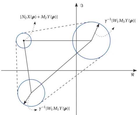
Ω=16 closed-loop responses are for all possible combinations of the time delay parameters in (A.22). . . 148 A.4 Gershgorin bands centered atLq q with the largest time delay combination in
(A.22): performance filter with|W1q| =0.5 (green circle), Gershgorin bands corresponding toq=1 (blue circles), Gershgorin bands corresponding toq=2 (red circles). Note thatZ(jω) is simply the complex number representation of each circle in the plot. . . 149 A.5 MIMO SP closed-loop response to a unit step input withτq p =ζq p ∀{p,q}:
reference signal (black,dash), output response with the proposed optimization method (blue, solid), output response with the “squared down" method. . . 151 A.6 MIMO SP closed-loop response to a unit step input withτq p=1.2ζq p∀{p,q}:
reference signal (black,dash), output response with the proposed optimization method (blue, solid), output response with the “squared down" method. . . 151 A.7 MIMO SP controller output response to a unit step reference: Controller output
response of proposed method withτq p=ζq p(blue, solid), controller output re-sponse of “squared down" method withτq p=ζq p(red, solid), controller output response of proposed method withτq p=1.2ζq p(blue, dash), controller output response of “squared down" method withτq p=1.2ζq p(red, dash) . . . 152
3.1 Procedure for optimizing low-order controllers. . . 41 4.1 Procedure for computing anRST controller . . . 60 4.2 Parameters resulting from the bisection algorithm. . . 66 5.1 Procedure for computing a controller withH∞performance (with respect to
the fundamental frequency of a sector-bounded nonlinearity) . . . 90 6.1 Procedure for executing the PSO algorithm . . . 105 6.2 Comparison of optimal solutions from convex and non-convex problems (with
optimization time) . . . 108 6.3 Comparison between optimal solutions and optimization time for multi-model
problem . . . 110 7.1 Procedure for obtaining local optimal solution with convex formulation . . . . 118 7.2 Optimization results forH2andH∞problems . . . 124 7.3 Performance for different optimization criteria . . . 126 7.4 Performance values for all methods . . . 132
1.1 Motivation
1.1.1 Brief History on Automatic Control
The initial use and implementation of feedback control is claimed to have originated from the Hellenic worlds; the earliest known construction of a feedback control mechanism was an ancient water clock invented by a Greek mechanician named Ktesibios in the third century B.C. [1]. The invention of devices for automatic control of temperature (i.e., the thermostat) and windmills were established in the 17thand 18thcentury. The flyball governor (initially conceptualized by James Watt in 1788) was a feedback system that implemented the principle of proportional control to regulate steam engines; an analysis of this type of system was performed by James Clerk Maxwell [2]. This system led to an uprising in the art of modern control theory which sprouted the industrial revolution. The increased use of engines in the modern era led to further investigation of feedback control by Bode [3] (who introduced the notions of gain and phase margins) and Nyquist [4] who published his celebrated frequency-domain encirclement criterion. Poincaré and Lyapunov also published important works in modern and state space approaches.
As time progressed, the emergence of other sophisticated control algorithms of feedback systems have been devised in response to the technological advances of industrial settings. The introduction of digital technologies in the late 1950s brought enormous changes to automatic control. Digital computers made it possible to implement more advanced control algorithms that were being developed in the 1970s [5]. Control methods such as adaptive control have a long history; however, it was the digital computer which offered the advantage of identifying the system parameters, making decisions about the required modifications to the control algorithm, and implementing the changes in a timely manner. Optimal and robust control techniques (such as model-predictive-control (MPC), linear-quadratic-Gaussian (LQG) and H∞approaches) could not be realized for practical applications without the help of digital computers [6]. However, at that time, computers were not sophisticated enough to solve such problems in a reasonable manner and solutions for these problems were attempted
to be derived analytically (which was a very difficult task). However, as time progressed, technological advances were made in the computing world which allowed computers to solve these problems very efficiently. As our increasingly advanced technologies enable us to build larger, more capable, more complex systems, the role of design becomes ever more important. Due to the complexity of many of today’s industrial processes (transportation systems, aerospace systems, communication systems, etc.,), the modeling of these systems by using first principles may be impossible. Even though a physical model is available, these models tend to be too complex for analysis and controller implementation. Data-driven control schemes seek to alleviate this problem by synthesizing controllers without the need of a physical model.
1.1.2 The Data-Driven Paradigm
In industrial schemes, the dynamics of plants are typically approximated by low-order models, since the controller synthesis is easier to implement for lower order processes. However, this approximation can impede the performance of a controller, since low-order models are subject to model uncertainty. In a data-driven design setting, a controller is designed by directly using online or offline input/output data (instead of designing a controller based on first modeling of a given plant). Data-driven methods aim to design controllers through direct usage of the process data while eliminating the challenging and tedious issues associated with the modeling process. In this manner, stability and performance can still be guaranteed under certain reasonable assumptions. A survey on the differences associated with model-based control and data-driven control has been addressed in [7] and [8]; the authors assert that model-based control methods are inherently less robust due to the unmodeled dynamics of a process, and that these controllers may possibly be unsafe for practical applications. With the data-driven control scheme, the parametric uncertainties and the unmodeled dynamics (for linear time-invariant systems) are irrelevant and the only source of uncertainty comes from the measurement process.
Given the available resources of a digital computer, access to huge amounts of measured process data can easily be collected due to the well-developed information technology (i.e., collected information from stored historical data or online data in real-time during process runs). The information can be collected and interpreted in the time-domain or frequency-domain. The frequency-domain approach offers many advantages compared to time-domain methods:
• Without knowledge of the transfer function, the dynamics of a system can be captured experimentally through the frequency response.
• Relative and absolute stability of a closed-loop system can be determined with the knowledge of the open-loop frequency response.
analysis.
• Frequency-domain analysis can also be carried out for nonlinear systems (including systems with strong nonlinearities such as chaos and bifurcation [9]).
In addition to avoiding the problem of unmodeled dynamics, the use of controllers with pre-defined structures is also important. In the classical robust control design method, the order of the resulting full-order controllers can be quite large; in fact, the order can be as large as the order of the augmented plant [10]. This can be problematic since it is known that computers possess cost-limited hardware and are limited in computing resources. However, the increased dependency on computers for control systems has fostered a need for control designs in a digital framework. Thus the notion of fixed-structure controller synthesis becomes an important subject in today’s controller design scheme. In fact, the proportional-integral and proportional-integral-derivative (PI/PID) controllers are still the most widely used controller structures in today’s industry due to their ease of implementation. It is known that more than 90% of all control loops are PID [11].
Fixed-structure robust controller design schemes for linear systems (in a data-driven setting) have been the focus of ongoing research. To a certain degree, the effects of nonlinearities could be ignored because they did not impair system performance. However, due to the increased performance demands on today’s industrial systems, the effects of certain nonlinearities can impact the behavior of these systems. For many of today’s systems, the effects of nonlinearities can no longer be neglected (see [12] and [13]). Due to the extensive use of frequency-domain techniques for linear systems within the control systems community, and given the need for analyzing the effects of nonlinear systems, it is thus natural to extend the frequency-domain analysis and control schemes for linear systems where nonlinear distortions can occur. A comparative study of frequency-domain methods for nonlinear systems has recently been addressed in [14].
1.2 State of the Art
In this section, a review of the current literature on data-driven control schemes that include fixed-structureH2andH∞design methods for linear systems is presented, as this is one
of the major research topics covered in this dissertation. Additionally, a review of nonlinear controller design methods (using frequency-domain data) is also presented.
1.2.1 Data-driven Control
Data-driven controller design is a very attractive research field within the control community (see [8, 7, 15]). In this method, a controller is designed by using either the time-domain or frequency-domain data of a system rather than using a parametric model of the plant (where the intermediate identification procedure or first principle modeling is not required).
A comparative analysis shows that although model-based approaches are statistically more efficient in terms of the variance of the controller parameters, a data-driven approach can outperform the model-based approach in terms of the final control cost [16]. Data-driven controllers can be synthesized either on-line or off-line.
On-line Methods
On-line methods refer to design schemes where the parameters of a controller are adjusted in real-time while the system is running in closed-loop operation. The classical model-reference adaptive control (MRAC) [17] may be considered as the first data-driven attempt to solve the model-reference problem in an on-line manner. This method attempts to minimize the tracking error and adjust the controller parameters from an on-line identification of the process model.
Model-free adaptive control (MFAC) [18] is a more recent data-driven approach that imple-ments a dynamic linearization of the process whose controller design and stability analysis merely depend on the measured input and output data of the controlled plants. This method can be used to design discrete-time controllers for nonlinear systems and multiple-input-multiple-output (MIMO) processes [19, 20]. More recent extensions and applications which implement this method can be found in [21, 22, 23, 24].
Unfalsified control (UC) [25] is yet another on-line control strategy which uses a fictitious reference signal to control a closed-loop system. The unfalsified control theory views the control problem as an identification problem where a control law is identified based on control performance goals, problem constraints, and evolving observational data. With this method, a controller is discarded when the fictitious signals do not satisfy the desired specifications. A non-iterative approach for controller design using unfalsified control is presented in [26]; however, this method is limited to stable systems. [27] extends on the concepts of unfalsified control by using Riccati-based parameterization ofH∞controllers. Note that an off-line non-iterative method for UC has recently been proposed in [28].
Off-line Methods
Off-line design schemes can synthesize controllers before they are applied to a system. Thus when there is no need for adaptation (and the process is time-invariant), these methods are favorable due to their ease of implementation. However, these methods rely on finite amount of data that is generated from a given identification experiment. The widely used PID controller is usually tuned based on a set of time-domain or frequency-domain data. The first examples of automated tuning using PID controllers were based on empirical methods proposed by Ziegler and Nichols [29].
Iterative feedback tuning (IFT) [30, 31] is an offline control methodology that uses an iterative technique to solve a non-convex problem to obtain the controller parameters; this method can
consider fixed-structure controllers. The main goal is to obtain unbiased gradient estimates and optimize for time-domain performance. The gradient of a criterion (with respect to the controller parameters) is computed such that a desired specification is satisfied (which is usually accomplished by minimizing a desired performance criterion). A typical performance criterion is to minimize the error between the reference signal and the actual output. The controller parameters are updated based on data obtained from multiple experiments. How-ever, stability is not guaranteed with this method. Some works which devised robust stability conditions for the IFT method are asserted in [32, 33], and recent applications of robust IFT controller design methods have been addressed in [34, 35].
The virtual reference feedback tuning (VRFT) [36] is an offline one-shot method which min-imizes the (filtered)H2norm of the difference between a desired reference model and the achieved closed-loop system. In this method, a controller is computed based on the mea-sured plant input when fed by a “virtual” error. This signal is computed assuming that the experiment was “virtually” performed in closed-loop with the controller achieving the desired specifications based on a given reference model. This idea was first proposed in [37], where it was denoted as Virtual Reference Direct Design. The authors in [38] give an overview of data-driven methods for the generalH2control problem. Recent developments and extensions using the VRFT technique for SISO systems ([39],[40]) and MIMO systems ([41],[42],[43]) have also been studied.
Iterative Correlation based Tuning (ICbT) [44] is another off-line approach where the objective is to adjust and fine tune the controller parameters by decorrelating the closed-loop output error and the reference signal. It implements the concepts of system identification where the predictor of the plant output is adjusted to make the prediction error uncorrelated with the plant input. An extension of this method to MIMO systems has been presented in [45]. However, in [46], a correlation-based tuning (CbT) approach is presented (which is a non-iterative version of ICbT) where the stability issue and the influence of measurement noise in the model-reference problem are studied.
A comparative study of different data-driven model-reference methods for non-minimum phase plants has been recently given in [47]. Note that VRFT, IFT, CbT, and the unfalsified control strategies are model-reference based schemes; these types of problems require special care since minimization of a desired reference model can lead to poor stability and robustness margins.
1.2.2 Fixed-Structure Controller Design
Controller synthesis methods belonging to theH∞control framework minimizes theH∞ norm of a weighted closed-loop sensitivity function. In the generalH∞synthesis problems, controllers are computed using semidefinite programing (SDP) algorithms [48] or algebraic Riccati equations [49]. The solutions of theseH∞control problems refer to the full-order case (which are convex). The controllers that result from these algorithms, however, are
typically of very high order, which complicates implementation. As discussed above, due to the ease of implementation of low-order controllers (such as the PID) and the limited computational resources of today’s embedded systems, the control engineer is confined to design fixed-structure controllers. It is well known that fixed-structure controller design in the model-based setting is a non-convex optimization problem. In fact, some of the problems in [49] for fixed-structure controllers are regarded as NP-hard [50], which makes theH∞ problem (with fixed-structure controllers) an inherently difficult problem to solve. Non-smooth optimization methods for fixed-structure controllers are used in [51], [52] and [53]; these methods are implemented in theMATLABRobust Control Toolbox (which is called with thehinfstructcommand). In parallel, a code package for fixed-order optimization called
HIFOOwas being developed that considered the same non-smooth problem formulation as [51], but can considerH2synthesis as well. However, these non-smooth techniques cannot synthesize controllers based on the frequency response of the system (they need a parametric model), and are limited to certain system dynamics (i.e., a pure delay must be approximated by a Padé function).
Design Using Frequency-Domain Data
Frequency-domain based controller synthesis methods are design schemes that continue to spark the interest of many researchers. Controller design methods which synthesize controllers by only using the frequency-domain data of a process can be categorized as a data-driven control scheme (since no parametric model is used for the actual synthesis). Therefore, given the fact that the modeling process for today’s systems is inherently problematic, it is natural to implement and develop a data-driven design methodology to design robust controllers. A robust frequency-domain controller design method has been established in [54]. In this method, upper and lower bounds are set on the desired closed-loop specifications where rational controllers are computed; however, this method requires a solution to a nonlinear optimization problem. Additionally, closed-loop stability is not guaranteeda-priori. Another frequency-domain loop-shaping approach to design fixed-structure controllers is presented in [55]. In this method, a convex optimization problem can be formulated if a linearly pa-rameterized (LP) controller is considered; however, as in [54], the closed-loop stability is not guaranteed and should be verifieda-posteriori. A more recent loop-shaping method has been proposed in [56] where the authors address theH∞problem for stable SISO and MIMO systems. The authors impose multiple line constraints in the Nyquist diagram to achieve both the closed-loop stability and performance. Feasibility constraints are proposed which are multilinear when LP controllers are used; for special controller cases, the feasibility constraints become convex.
In [57], a frequency-domain approach is realized where a convex optimization algorithm is formulated by considering a convex approximation of theH∞criterion. The constraints are convexified around a desired open-loop transfer function where a non-iterative algorithm is proposed to optimize a set of LP controllers that guarantee the closed-loop stability. This
method is extended to data-driven gain-scheduled controller design in [58] and multivariable decoupling controller design in [59]. A toolbox that implements the methods used in these works has been devised in [60].
In [61, 62], a frequency-response method is proposed based on theQ-parametrization to guarantee theH∞performance for fixed-structure controllers. This method linearizes the non-convexH∞constraint using a first-order Taylor expansion around an operating point; in this manner, the local solution to the fixed-structureH∞problem is obtained. An ini-tial stabilizing controller is needed in order to guarantee the closed-loop stability. Another frequency-domain approach for computing LP controllers is presented in [63] where theH∞
constraints are convexified around an initial stabilizing controller; an iterative algorithm is used that converges to a local optimal solution of the non-convex problem. In [64], the authors also linearize a non-convex constraint around an initial stabilizing controller and implement an iterative method for obtaining a local solution; however, in this work, the objective was to minimize the integrated error underH∞robustness constraints. The convex-concave approximation of theH∞constraint in [64] leads to the same constraint as in [57] for PID controllers. The extension of this method to design multivariable PID controllers for stable systems is presented in [65] (where the linearization is performed with respect to a quadratic matrix inequality). More recent works that implement an iterative method that ensuresH∞ performance have been devised in [66]. The non-convexH∞constraints here are also lin-earized around an initial stabilizing controller, but the method is not limited to LP controllers and stable systems and can considerH2performance as well.
1.2.3 Nonlinear Control
In principle, all real-world systems are nonlinear and it would seem appropriate to consider nonlinear control theory for real applications. In general, it is very difficult to generalize a controller design method to apply to all nonlinear systems; thus various theories have been developed by considering specific classes of nonlinear systems. The limit cycle theory, Poincaré maps, Lyapunov stability theory, and describing functions are some methods that are used for stabilizing and controlling systems that include specific classes of nonlinearities. The theory of nonlinear control is very broad; in this dissertation, the focus is placed on nonlinear control using theH∞criterion and in a data-driven setting (as this is the framework of this dissertation).
H∞Control of Nonlinear Systems
There are many works that have addressed theH∞problem in the linear framework; however, only several works have been established forH∞control of nonlinear systems. In [67], a solution of the problem of disturbance attenuation with internal stability via measurement feedback is presented. The authors in [68] derived the necessary conditions for the existence of an output feedback controller such that the Hamilton-Jacobi-Isaacs (HJI) equations related
to the closed-loop system have a positive smooth solution; they confirmed the separation principle for the nonlinearH∞control problem (although stability was not guaranteed). The HJI equations are a set of nonlinear partial differential equations which in general cannot be solved analytically [69]. The solution to these equations give necessary and sufficient optimal control conditions for systems modeled by nonlinear dynamics. When the system is LTI, the HJI equations reduce to the familiar algebraic Riccati equations (AREs). The work in [70] implements a Galerkin approximation to obtain the solution of the HJI equations forH∞ control. In [71], state-dependent Riccati equation (SDRE) techniques are used in an iterative fashion (i.e., by solving a set of convex optimization problems) to approximate the solution of the HJI equations and obtainH2orH∞performance. SDREs, however, are computationally expensive where convergence to a solution may take significant time. The recent work in [72], however, proposed an update algorithmin a data-driven settingto learn the solution of HJI equations iteratively and provide a convergence proof.
Data-Driven Control of Nonlinear Systems
Data-driven methods for controlling systems with nonlinearities is a field which continues to grow and evolve. The describing function (DF) method was first conceptualized by the authors in [73] and is one of the few widely applicable methods for analyzing a certain class of nonlinear systems. This method uses the frequency response method for analyzing linear systems that are subject to time-invariant odd nonlinearities. DFs approximate the dynamics of a nonlinearity by only considering the fundamental component of the nonlinear response; the justification for considering only the fundamental component is made by the fact that for real physical systems, the linear subsystem of the overall nonlinear system is a low-pass filter which attenuates the higher frequency components of the nonlinearity. In this manner, an approximate model can be formed for the nonlinearity. Some recent works and applications using the DFs are proposed in [74, 75, 76]. The DF method, however, can fail badly for systems which emphasize higher harmonics of the nonlinearity. Some examples of this have been presented in [77] for bang-bang systems.
More recent data-driven methodologies for controlling nonlinear systems have also been studied in the literature. The authors in [19] present a model-free approach to design con-trollers that guarantee stability for a class of nonlinear discrete-time systems; in [20], this method is extended to the MIMO nonlinear system. A VRFT method is proposed in [78] to design controllers for nonlinear plant models using a direct “one-shot" method. The authors in [79] build on the iterative learning control data-driven algorithm to design controllers for a class of nonlinear autoregressive exogenous models. A method for designing controllers in a data-driven setting for constrained linear systems is presented in [80]. A specific 2-degree-of-freedom (2DOF) controller structure is used in [81, 82] where a nonlinear controller is used in parallel with a linear controller to control nonlinear systems by using the VRFT design approach. The work in [83] extends on the concept of the VRFT method and implements a data-driven scheme to design linear parameter-varying (LPV) model-reference controllers.
Frequency-domain methods for stabilizing systems with nonlinearities has also been inves-tigated in literature. One of the most remarkable theories in systems and control theory is the Kalman – Yakubovich – Popov (KYP) lemma [84, 85], which established the equivalence between frequency-domain conditions (e.g., Circle and Popov criteria) and time-domain con-ditions for absolute stability of Lur’e systems. The Circle and Popov criterion have proposed frequency-domain methods that stabilize systems with sector-bounded nonlinearities. There are many variations of these theories that have been recently proposed in literature to control nonlinear systems [86, 87, 88, 89, 90, 91, 92].
1.3 Research Objectives
1.3.1 Global Solution ofH∞problem
The first objective of this dissertation is to implement a data-driven method (using frequency-domain data) and develop a convex optimization problem such that the global optimal solu-tion to theH∞problem is obtained. Formulating convex problems are desired since (1) they are computationally tractable, and (2), a convex objective function ensures that all local optima are global optima [93]. Many works have been published for optimizing LP controllers using frequency domain-data and convex optimization algorithms. In these works, LP controllers were specifically chosen since this convexifies theH∞problem.
In this dissertation, it is desired to develop a necessary and sufficient (convex) condition for attainingH∞performance while guaranteeing the closed-loop stability of a system (using controllers that are not LP where a controller’s numerator and denominator are simultaneously optimized). By convexifying theH∞problem, the global solution to an approximate problem is obtained; given the necessity and sufficiency of the convex problem, the solution to the convex problem will converge to the global optimal solution of the trueH∞problem as the controller order is increased.
The outcome of the objective asserted in the previous paragraph is based on systems with 1-degree-of-freedom controller structures in a continuous-time framework. Since the pro-posed method in this dissertation implements a data-driven frequency-domain approach for controller synthesis, it is natural to extend the above controller design methodology for
• systems using a 2-degree-of-freedom controller in a discrete-time framework • systems which are corrupted by nonlinear distortions
• systems which require constraints on multiple sensitivity functions
It will be desired to implement the proposed data-driven methodology to a particle accelerator power converter control system at CERN. In this system, the controller structure is fixed with a 2-degree-of-freedom discrete-timeRST controller; this type of controller is implemented
due to the fact that these systems require both very precise tracking capabilities and sufficient robustness margins.
The next objective is to further extend the proposed design methodology to nonlinear systems with sector-bounded nonlinearities. The Circle criterion provides a necessary and sufficient condition for stabilizing this class of nonlinear systems; thus the data-driven scheme can be combined with the ideas presented by the Circle criterion to achieve closed-loop stability. The main objective, however, is to formulate necessary and sufficient (convex) feasibility conditions for achieving the desired stability requirements.
1.3.2 Fixed-Structure Controller Design
With the objectives asserted in the previous subsection, it is evident that although convergence to the global optimal solution of theH∞problem is obtained with increasing controller order, the solution may be far from optimal for low-order controllers (since the global solution to anapproximate problem is obtained). Thus the next research objective is to optimize the controller performance for low-order controllers using frequency-domain data (while guaranteeing the closed-loop stability of the system); this can be accomplished by finding a local solution to theH∞problem using fixed-structure low-order controllers. Two methods are proposed for achieving this specification:
• Solve a non-convex problem (in a data-driven setting) to obtain a local solution to the fixed-structureH∞problem.
• Solve a set of convex problems in an iterative fashion (in a data-driven setting) to obtain a local solution to the fixed-structureH∞problem
Note that the objective here is to optimize non-LP fixed-structure controllers. In the previous subsection, the objective was to formulate a convex problem using non-LP controllers; the solution to this convex problem, however, does not guarantee that the local solution to the H∞problem (for fixed-structure low-order controllers) is obtained. Thus the main
differ-ence between the objective here and the objective discussed in the previous subsection is that convergence to a local solution for a given controller order is desired.
The non-convexH∞constraints do not guarantee the closed-loop stability of a given system; thus it is desired to formulate a non-convex problem which optimizes all of the fixed-structure controller parameters while guaranteeing the closed-loop stability. It is known that non-convex problems are difficult to solve since the quality of solutions depend heavily on the initial conditions. Thus a particle swarm optimization (PSO) algorithm is presented to solve this problem; PSO is a powerful optimization method that can solve both linear and nonlinear problems and can be used to solve problems without specifying initial conditions. However, when the problem is of large dimension, the quality of the solution or the optimization time can be inadmissible. Thus it is desired to compare the local solutions obtained from the
non-convexH∞problem and the convexH∞problem (for fixed-structure non-LP controllers, linearized around a stabilizing operating point) to determine the validity and practicability of both methods.
The fixed-structure design is implemented on the same CERN converter that was discussed in the previous subsection, but with a different load and a different reference signal to track. The local solution to the fixed-structure problem is obtained using the convex formulation since (1), this method can consider other performance criterion (i.e.,H1andH2performance), and (2), the method is more efficient in a computational sense.
1.3.3 Contributions
The following main contributions of this dissertation are highlighted as follows:
• It derives the necessary and sufficient conditions for achieving robust stability and ro-bust performancein a data-driven settingby minimizing the infinity norm of a weighted sensitivity function. The designed controller is robust with respect to the uncertainties captured in an identification experiment (which can be modeled as additive uncertain-ties).
• It derives the necessary and sufficient conditions for a certain class of models with frequency-domain polytopic uncertainties that are caused by measurement noise or multi-model incertitude.
• It shows that the solution to a convex problem converges monotonically to the global solution of the trueH∞problem as the controller order increases (while guaranteeing the closed-loop stability).
• It proposes a method to design controllers for linear systems that are subjected to nonlinear distortions.
• It derives necessary and sufficient conditions for stabilizing systems with sector-bounded nonlinearities. It also derives a sufficient condition for guaranteeing the closed-loop performance for all uncertain gains within the sector nonlinearity.
• It presents a method for obtaining the local optimal solution of theH∞problem for fixed-structure controllers. This method uses a PSO algorithm for achieving the solution in a data-driven setting.
• It proposes a convex model-reference problem for fixed-structure non-LP controllers where local optimal solutions to theH2orH∞problems are obtained. Closed-loop
stability of the system is guaranteed with a given initial stabilizing controller. It also proposes a method for obtainingH1performance.
1.4 Dissertation Structure
The structure and general layout of this dissertation is now provided. Since the class of models and controllers vary from chapter to chapter, a dedicated chapter has been inserted in order to clarify all of the class of models and controllers that are presented in this work.
Chapter 2: Preliminaries
This chapter is dedicated to defining all of the class of models, uncertainties, and controllers that are used throughout the paper.
Chapter 3: RobustH∞Controller Design
This chapter deals with the problem of robust stability and robust performance for LTI-SISO systems. Necessary and sufficient conditions are derived for guaranteeing the stability of the closed-loop system andH∞performance. A convex optimization problem is formulated in which a controller is parameterized as a ratio of two LP transfer functions; in this manner, the controllers numerator and denominator are optimized. It is shown that as the controller order increases, the global optimal solution to theH∞problem is obtained. The robustness of the closed-loop system is established by considering an additive uncertainty of coprime factors (which can be easily obtained by spectral analysis of measured data). With this method, conditions for ensuring the performance and stability for systems with frequency-domain polytopic uncertainties are also derived. The simulation and experimental results at the end of the chapter show the effectiveness of the proposed method.
Chapter 4: RST Controller Design for Particle Accelerator Power Converters
In this chapter, the necessary and sufficient conditions for obtaining<