Partition-based Model Representation Learning

(1)

Yayun Hsu

Submitted in partial fulfillment of the requirements for the degree of

Doctor of Philosophy under the Executive Committee of the Graduate School of Arts and Sciences

COLUMBIA UNIVERSITY

(2)

(3)

Abstract

Representation Learning – A Partition-based Model Approach Yayun Hsu

Modern machine learning consists of both task forces from classical statistics and modern computation. On the one hand, this field becomes rich and quick-growing; on the other hand, different convention from different schools becomes harder and harder to communicate over time. A lot of the times, the problem is not about who is absolutely right or wrong, but about from which angle that one should approach the problem. This is the moment when we feel there should be a unifying machine learning framework that can withhold different schools under the same umbrella. So we propose one of such a framework and call it “representation learning”. Representations are for the data, which is almost identical to a statistical model. However, philosophically, we would like to distinguish from classical statistical modeling such that (1) representations are interpretable to the scientist, (2) representations convey the pre-existing subject view that the scientist has towards his/her data before seeing it (in other words,

representations may not align with the true data generating process), and (3) representations are task-oriented.

To build such a representation, we propose to use partition-based models. Partition-based models are easy to interpret and useful for figuring out the interactions between variables. However, the major challenge lies in the computation, since the partition numbers can grow exponentially with respect to the number of variables. To solve the problem, we need a model/representation

(4)

selection method over different partition models. We proposed to use I-Score with backward dropping algorithm to achieve the goal.

In this work, we explore the connection between the I-Score variable selection methodology to other existing methods and extend the idea into developing other objective functions that can be used in other applications. We apply our ideas to analyze three datasets, one is the genome-wide association study (GWAS) [1], one is the New York City Vision Zero [2], and, lastly, the MNIST handwritten digit database [3].

On these applications, we showed the potential of the interpretability of the representations can be useful in practice and provide practitioners with much more intuitions in explaining their results. Also, we showed a novel way to look at causal inference problems from the view of

partition-based models.

We hope this work serve as an initiative for people to start thinking about approaching problems from a different angle and to involve interpretability into the consideration when building a model so that it can be easier to be used to communicate with people from other fields.

(5)

List of Figures

1.1 Example of a hierarchical representation of a cat. . . 4

2.1 Illustration of the structure of an ANN. . . 16

2.2 A data generating process example. . . 20

3.1 An illustration of representation learning. . . 32

3.2 Latent variable model. . . 32

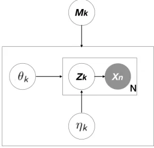
4.1 Data generating assumption. . . 38

4.2 Proposed decomposition of representation learning. . . 38

4.3 Data generating process assumption (unsupervised). . . 40

4.4 Partitions ranked by the proposed procedure. . . 44

4.5 Histograms on the number of partitions. . . 45

4.6 Intuition for the partition selection mechanism. . . 46

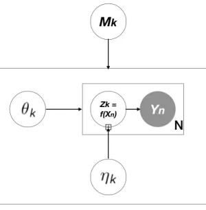
4.7 Data generating process assumption (supervised). . . 48

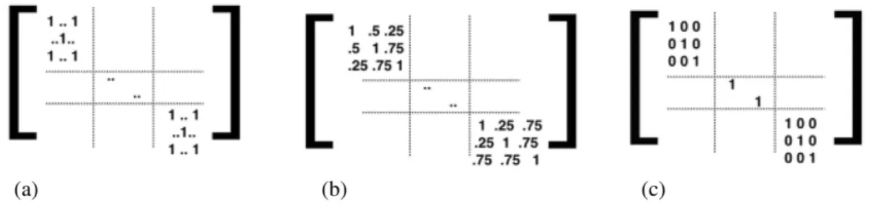
5.1 Kinship coefficient matrices used in 3 modeling options for fitting the linear mixed-effects model to data with family structures. (a) Option 1: representatives. (b) Option 2: kinship. (c) Option 3: independent. . . 59

5.2 Ideal relation among significant SNP sets from 3 different modeling options. . . 60

(11)

5.4 Manhattan plots for option 2 and option 3 (black dots). . . 61 6.1 The comparison between case and control without any conditioning. . . 90 6.2 The comparison between case and control conditioned on borough. . . 91 6.3 The comparison between case and control conditioned on the date when enhanced

crossings were built. . . 92 6.4 The comparison between case and control conditioned on if the corridor was

pri-oritized. . . 93 6.5 The comparison between case and control conditioned on if the zone was prioritized. 93 6.6 The comparison between case and control conditioned on the date when slow zones

were built. . . 94 6.7 The comparison between case and control conditioned on the borough and the

prioritized corridor. . . 95 6.8 The comparison between case and control conditioned on the slow zone and the

prioritized corridor. . . 96 6.9 The final partitions chosen from I-Score procedure. . . 97 7.1 Deep artificial neural network as hierarchical representation learning. . . 100 7.2 The encoder compresses data into a latent representation, and the decoder

recon-structs the data given the hidden representation. . . 101 7.3 GAN architecture. . . 106 7.4 BiGAN architecture. . . 107 7.5 The latent space learned from VAE and Info-BiGAN with different p(z). Top:

VAE; Middle: Info-BiGAN with Normal prior; Bottom: Info-BiGAN with Uni-form prior. . . 111 7.6 Generated hand-written digits from Info-BiGAN. . . 112

(12)

Chapter 1: Introduction and Background

1.1 Motivation

Machine learning is the intersection where many disciplines meet, especially Statistics and Computer Science. Modern machine learning suffers from the trade-off between inference and prediction [4]. 1 For example, in traditional statistical linear regression, under the normality as-sumption, the model learned from maximum likelihood gives us direct inference results on the coefficients. If one attempts to use the resulting model for predicting out-of-sample future obser-vations, it is usually not the best, compared with other methods such as nonparametric regression, kernel methods, or even neural networks. However, the current solution to this problem is a mat-ter of choice – practitioners are forced to choose sides between these two cultures, without other middle-ground option(s). In this work, we would like to propose a new learning framework, which we will call it the “representation learning”, that acts as another option other than traditional sta-tistical modeling and black-box modeling.

From a statistical viewpoint, many modern machine learning methods are the retell of stories from earlier statistical toolbox with the aids of modern computation. As a statistician, I am glad to see how modern computation elevates statistics to a new scale that statisticians would never had imagined a few decades ago. From Computer Science (and even Artificial Intelligence) standpoint, researchers are thrilled to see the idea of learning a prediction model from past data, instead of human hard-coded rules, has opened a whole new world of problem-solving regimes. For example, AlphaGo, the first computer Go program to beat a human professional Go player, is based on modern deep-learning systems, instead of hard-coded systems such as Deep Blue2that appeared

1_{Throughout this work, we will refer to the former as the traditional statistical model, and the latter as the black-box}

model, following the same naming of Breiman.

2_{the first computer chess-playing system to win both a chess game and a chess match against a human reigning}

(13)

nearly 30 years ago.

As a result, we have seen almost exponential growth in machine learning because of the joint contribution of great minds from various disciplines. However, this rapid development is not with-out a price – if we look at modern, computational-approached methods through a statistical lens, many of them are not explainable, and even violate some statistical principles; however, they per-form well in practice. For example, a regression coefficient is not a causal estimate unless a large set of assumptions are met. But in practice, many assumptions are actually uncheckable. In those cases, do we give up the methods entirely? Do we still apply the methods blindly? Or are there any other choices?

Given the rich developments and successes on both sides, instead of trying to deny their dif-ferent mindsets entirely, we feel the need to construct a new framework, where people from the two sides of the spectrum can meet and share a common language. Hopefully, by constructing this bridge, people will be able to understand and appreciate what each other has been doing, thus helping the further development of each.

1.2 Representation Learning

The solution that we propose here, the new learning framework that we will construct, will be called representation learning. Indeed, the term “representation learning” has been around for quite a while, but there is no unifying definition for it. From Computer Science community, repre-sentation learning has become a field in itself, with regular workshops at the leading conferences such asNIPSandICML, and a new conference dedicated to it, theICLR(International Conference on Learning Representations), sometimes under the header of Deep Learning or Feature Learn-ing. The rapid increase in scientific activity on representation learning has been accompanied and nourished by many empirical successes both in academia and in industry [5]. Fields such as signal processing, natural language processing, object recognition, and transfer learning, have all seen benefits from representation learning.

(14)

my goal is to borrow the name and to set up a new learning framework that was described in the previous section. Throughout the whole thesis, I will focus on (1) setting up the framework, (2) providing a proper loss function/ objective function, and (3) interpreting the results and implica-tions.

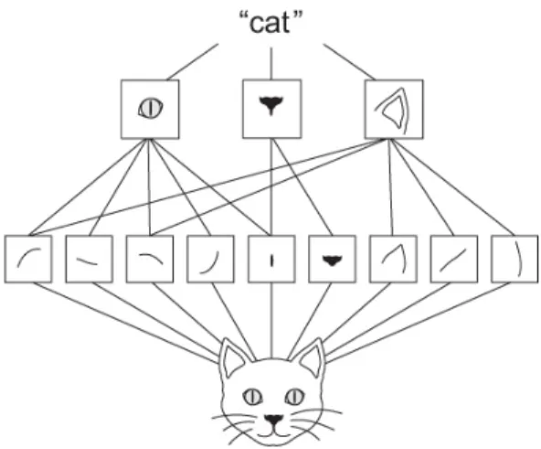
First of all, we define representations to be hierarchies of decompositions or transformations of the raw data such that some of them are useful for some tasks. There are generous-purposed representations and specific-tasked representations. Let me explain these qualitative properties of representations using an intuitive example. Figure 1.1 illustrates the idea – we are given a bunch of pictures of cats, which is the observable data. In representation learning, we abstract the pictures of cats into hierarchies of representations. The two ends of the hierarchical representations are the data (in this example, the picture of the cats) and the task (in this example, predicting the label “cat”). The data is observable; the label may be observable or not. Furthermore, the label can change domains – the same picture of a cat can be labeled as “cat”, “animal”, “happy”, “summer” or “black-and-white”, etc. Between the data and the label, several hierarchies of representations can be constructed. The first layer above the raw data is for more generous purpose; as the layers move towards the label, those layers become more and more specific for the “task” – predicting the label. Here all the inner layers are legitimate representations, but not all of them are useful for all tasks. For example, if the task is to distinguish a cat from a dog, then probably the color of the picture doesn’t help much; while if the task is to distinguish in which season the picture was taken, then color becomes an important representation.

I will use the term “task” to include most of the problems considered in machine learning, involving prediction, estimation, variable selection, etc.

We will see later that, using this proposed learning framework, we will be able to achieve (1) good interpretation (2) prevention of overfitting, and (3) variable selection all at once.

As discussed previously, the purpose of constructing such a framework is to give a common language to both sides of the culture. So in the following sections, I will explain how to use this newly defined “representations” to look at some traditional statistical models.

(15)

Figure 1.1: Example of a hierarchical representation of a cat. 1.2.1 Linear Regression as Representation

Suppose we have data(Yi,X_i1,X_i2, ...X_ip), wherei denotes the index for observations andp

de-notes the number of independent variables/ observed features. In the linear regression setting, we have model

Y = XTβ+, (1.1)

whereYis a known vector of observations with meanXβ,βis an unknown vector of constants,

is an unknown vector of random errors with mean 0 and variance R, and X is a known design matrix. We can view Equation 1.1 as a decomposition ofY into the signal XTβ and the noise parts. We callXTβ as the representation ofY under this model specification.

Traditionally in the modeling stage, the problem is that we don’t know (1) how many indepen-dent variables we should use and (2) even if we know the answer to (1), we still don’t know which variables compose the best subset. So many selection criteria have been proposed, such as AIC, BIC, and LASSO. On the other hand, from a black-boxed model point of view, if a better predic-tion accuracy can be achieved by adding more independent variables, there is no fault of doing so. It is a matter of the focus. In our proposed representation learning, we introduce a new focus – the interpretability of the representation. By interpretability, we mean the intuitive interpretation that we human can make sense about. In some cases, the interpretability may be obvious and even checkable in its own field knowledge. Such cases are like using random forests to build a

(16)

genome-wide prediction for a certain disease. In other cases, the interpretability may not be obvious – in these cases, one may still want to stick with traditional criteria.

Now let’s go back to the linear regression example, and elaborate more on the representation learning ideas. We know that, under the usual linear regression assumptions, the solution from ma-chine learning theory says that the predictedY is given byYˆ = (X(XTX)−1XT)Y = HY, where H is often called the hat matrix, and it stands for a linear transformation onY [6] [7]. In our proposed representation learning framework, we say this is the empirical representation ofY. This represen-tation is obtained through maximum likelihood estimation, so, by construction, it is interpretable for inference but may not for prediction. The interpretation is –Yˆ is a projection of the vectorY® onto the space spanned by X, and it is perpendicular to the residual vector,®; therefore, we have a orthogonal decomposition ofY into signal and noise.

However, in terms of prediction, as we know from machine learning theory that, for prediction purpose, it is often better to use slightly biased estimators obtained through penalization – this then becomes a black-boxed model. Is there another solution to the regression problem that can have both of the interpretability and the prediction accuracy?

Our proposed solution is that, linear regression can be done first by representation learning – this is the inference step that gives us interpretability – and then use the learned representations to build the prediction model. By doing so, we strike a balance between inference and prediction. Representation learning can use, for example, I-Score, principle component analysis (PCA), vari-ational autoencoder (VAE), etc. The I-Score variable selection procedure is the main route we will pursue in this thesis, and hence more detailed introduction will be present later. But the basic idea is that we first use I-Score to perform variable selection, and then use the selected variables to build regression models or neural networks.

(17)

1.2.2 Mixed (Hierarchical) Models as Latent Representation

An additive mixed model is a statistical model containing both fixed effects and random effects. In matrix notation, a mixed model can be represented as

Y = XTβ+ZTµ+, (1.2)

where whereY is a known vector of observations with mean XTβ, β is an unknown vector of fixed effects, µ is an unknown vector of random effects with mean 0 and variance–covariance matrixG, is an unknown vector of random errors with mean 0 and variance R, and X andZ are known design matrices relating the observationY toβand µ, respectively [8]. We will call X and Z as the “features” –X is the observable, raw feature, and Z is the latent feature (may or may not be observable).

In our representation learning language, we can view the above modeling as an additive, hier-archical decomposition of the observationY.

Y = µ0+σ00 | {z } µ1 +σ11 | {z } µ2 +σ22+...

assuming that eachiis independent with µ0.

The modeling of a hierarchical model suffers from similar issues as linear regression – since we don’t know how many hierarchies is “correct” (there may even not be a correct answer), we’d better first build representations in the inference step and then proceed with the model-building. The difference is that, sinceZ may be unobservable, it may require us to do some clustering onY in building the representations.

For demonstration purpose (and without loss of generality), let us study a two-level model, albeit the concept can be generalized to even higher levels of hierarchies.

(18)

Several results from this model construction:

E(Y)= µ0 (1.4)

Var(Y)= σ₀2+σ₁2+σ₂2 (1.5)

Cov(Y, µ1)= σ₀2 (1.6)

Cov(Y, µ2)= σ₀2+σ₁2 (1.7)

That is, even before we fit the model, we know the form of the variance-covariance structure. In some applications, such as kinship modeling, we can pre-assign the variance-covariance structure before fitting the model. This once again emphasizes the idea that an interpretable representation can go before model fitting, to ensure the learning results make intuitive sense in real applications.

1.2.3 Mixture Models as Representation

In mixture models, the whole population can be treated as a mixture of several mixture com-ponents. Since the mixture components are usually unseen, we refer to them as latent variables. The mixture components can be either discrete or continuous, but often for modeling convenience, they are assumed to be discrete. In general, a mixture model assumes the data are generated by the following process: first we sample from the latent variableZ, and then we sample the observables X from a distribution which depends onZ; that is,

p(x,z)= p(x|z)p(z), (1.8)

where p(x|z)is the representation based on latent components. Note that the above factorization doesn’t suggest any ordering. So it is important to determine the ordering in the representation building stage.

Let us first review how traditionally people fit these kinds of model. Assuming that the true model is a Gaussian mixture model on the marginal data X with mixture components Z. X is

(19)

observable while Z is not. We assumeZ is a discrete random variable, and there are probabilities defined onp(X|Z = k), for k ∈ {1,2, ...,K}, whereK is the total number of mixture components. Each p(X|Z = k) is Gaussian with mean µk and variance σ_k2. The parameters of interest are all

the µk,σ_k2andp(Z = k). We call each p(X|Z = k)the probabilistic representation of X based on

Z = k. If we follow maximum likelihood estimation for the parameters, there are two major issues: (1) different K may result in nonidentifiability, and (2) even ifK is fixed, the MLE objective has no analytical solution.

In practice, to resolve issue (1), people pre-select a fixedK. To resolve (2), a more traditional statistical method is the expectation-maximization algorithm (EM), while in recent years, Bayesian methods such as topic modeling and variational inference have become more and more popular [9]. However, it is often hard to determine how many mixture components there should be. Later we will see that the method of I-Score representation learning can actually serve as a method for determining the number of mixtures by specifying some sort of “prior belief”3.

On caveat is that, for a fixed dataset, there is no unique representation. It is simply because, representations are the subjective beliefs of the interpreter and they need not imitate the true data generating process, that we allow different practitioners to have their own representations, as long as they achieve the task well.

1.3 Partition-based Models

Here we define a partition over the feature space, where all features are discrete, is a collection of sets that (1) are mutually disjoint and (2) have a union as the entire composited feature space.

Suppose we have data (Y_i,X_i(1),X_i(2), ...X_i(p)), where i denotes the index for observations, p denotes the number of independent variables/ observed features, all the Yi’s are continuous and

all the X_i(p)’s are discrete. The partition of the feature space is defined on the composition of (X_i(1),X_i(2), ...X_i(p)). Assume that the partitions are {Π₁,Π2, ...ΠK}, where K stands for the total

number of partitions constructed.

(20)

The model we consider is

Yi =

Õ

k

µk·I(Yi ∈Πk)+i, (1.9)

where µkis the “local mean” ofY in partitionΠk, andiis the individual level error with mean

0 and independent with all other observations within the same partition, but may dependent with other observations across different partitions. The learning interests are all the local means µk and

the clustering procedureI(Yi ∈ Πk). We interpret all the local means µk as the representation ofY

under this partition-based model.

A partition-based model essentially clusters the observedY’s into these feature partitions. The desirable clustering should make observations inside each partition as homogeneous as possible. This has two consequences: First, we can then build local models within each partition, which yields a very expressive model. Second, we may find that some of the partitions contain no ob-servations inside, which further implies the irrelevancy of the variables used to construct those partitions. Hence, variable selection is also achieved in the process.

The hardest part of building such a model is the choice of objective function and the corre-sponding algorithm to automate the clustering process. These two will be the focus of this thesis – the I-Score objective function and the corresponding backward dropping algorithm [10] [11].

(21)

Chapter 2: Technical Approach

The procedures of our representation learning involve the following: (1) latent structure learn-ing of the predictors, (2) predictional modellearn-ing learnlearn-ing, (3) model checklearn-ing, and (4) result inter-pretation. For (1), we use the I-Score, proposed by Chernoff, Lo and Zheng [12], to serve as a variable selection tool. For (2), we use the generalized additive model (GAM) and neural networks as the basis. We will see that the model learned in this way has a natural interpretation. Some applications on the full implementation will be discussed in Chapter 5-7.

2.1 I-score

The setting of the problem is that we are given a dataset{(Y_i,Xi)}_iN₌₁whereNis the sample size. Although many variations have been proposed, here we stick to the setting thatY is a continuous random variable and all X’s are discrete. There may be a few features in X that is not useful for predictingY. We would like to sift them out, while not knowing what the true model is. The approach is to partition theN observations into several partitions, according to the composition of subsets of X withniobservations in theit h partition.

The composition of X is to redefine the high dimensional marginal X’s into a one dimensional variable that takes the joint value. For example, if we originally have two-dimensional(X₁,X₂)in the data, and each of the random variables can only take values either 0 or 1. We can composite (X₁,X2) into another random variable, say, X3, such that X3 can take four possible values that

correspond to the situation when(X₁,X₂) = {(0,0),(0,1),(1,0),(1,1)}, respectively. We call each one in the composite set a partition, as it is a partition over the feature space.

A great advantage of this model is that we take into consideration the joint distribution of the original X’s without making any implausible assumptions such as independence of the marginal

(22)

X’s.

However, the price for being able to take care of the joint distribution in X is that this kind of composite random variables can easily become sparse in the sense that there are many possible partitions that don’t have enough observations. So, instead of compositing all the raw features into one big new feature, we randomly sub-sample a few features and test their I-Score.

For a subset of X that compositesipartitions, the I-Score is defined to be

I = 1 N

Õ

i

n_i2(Y¯i−Y¯)2, (2.1)

where ni is the number of observations inside theit h partition, Íini = N, Y¯i is the average ofY

in theit h partition (local mean), andY¯ = Í

i niY¯i

N is the overall average ofY (global mean). It can

be a measure of influence based on how well the partition separates the subjects into relatively homogeneous subsets. It not only considers the deviation of local means to the global mean, but also take the number of observations inside each partition into account. The higher the I-Score, the more influential towardsY the set of features is.

One reason for explaining why partition models make such practical use is through local av-eraging. Many smoothers in nonparametric regression such as splines are known to be able to smooth the curve fitting by doing some kind of local averaging. However, the idea of locality becomes more and more vague as the dimension of features increases. This is the place where the partitions come in handy. In partitions, there is no ordering nor continuity. This methodology can then be related to tree-based methods, such as decision trees. However, the I-Score framework is different from trees in the sense that they take the interaction between features into account, by selecting a subset of features together at once; while in building decision trees, we only split the tree based on one marginal feature at a time.

Ideally, we would like to search over all possible subsets and find out the one with the highest I-Score. However, since the number of partitions grow exponentially with the number of features, it is impossible to do an exhaustive search in practice. Instead, they also proposed the backward

(23)

dropping algorithm [10] [11]. Essentially it is a greedy search that every time we drop one variable that has the minimum contribution to the score until we reach the peak value.

2.1.1 Backward Dropping Algorithm

Suppose in our data, we have pfeatures, X₁,X₂, ...Xp. The backward dropping algorithm is to

randomly select a subset of features from the total p features, and to evaluate the I-Score of the current subset by gradually dropping one feature at a time, until we find the maximum I-Score generated by a certain subset of the current random subset – this is how we drop the redundant variables. In each dropping stage, we perform greedy search – to drop the one variable that gives the highest decrease of I-Score in each iteration. The procedure is practical in many real data experiments [10] [11] [13].

2.1.2 Comparison

In a partition model, where we have the local meansY¯i and the global meanY¯ = ÍiniY¯i, we

have the following decomposition:

n Õ i=1 Yi−Y¯ 2 = n Õ i=1 Yi−Y¯i 2 + n Õ i=1 ¯ Yi−Y¯ 2_. (2.2)

In general, if we treat Equation 2.2 as a special case of the following equation, we can say that the local means in a partition-based model is an unbiased estimator for the response. So we have the following, n Õ i=1 Yi−Yˆ 2 = n Õ i=1 Yi−Yˆi 2 + n Õ i=1 ˆ Yi−Y¯ 2 . (2.3)

When we try to minimize Ín

i=1 Yi−Y¯i 2 , it is equivalent to maximize Ín i=1 Y¯i−Y¯ 2 , since their sum, the sample variance, is fixed. Without any restriction on the number of partitions, the minimum value of Ín

i=1

Yi−Yˆi

2

is zero; that is, by giving each datapoint its own partition. This is the same phenomenon of overfitting in linear regression. In linear regression, we prevent overfitting by restricting the functional form ofYˆi to be linear. On the contrary, in our proposed

(24)

partition-based representation learning, we prevent overfitting by choosing partitions that prefer more than one observations to be inside each partition. This is guided by using the I-Score as the objective function, since the I-Score is essentially the weighted version of the second term on the right hand side of Equation 2.2. The rationale of doing this is to guide the learning process to learn a meaningful, interpretable representation, instead of blindly optimizing the objective function. The representation here is that, inside each partition, the data are homogeneously i.i.d. In other words, the proposed partition-based representation learns a smoother representation than the normal regression, without being completely smooth (the null model of regression). On the other hand, it improves the typical objective functions used in tree-based learning methods by taking the interactions of the features into account, since, instead of finding marginal signal each time, one whole partition that consists of many variables is considered every time the in I-Score method.

In sum, if we see there is a spectrum of methods, one side of which is linear regression and the other side being tree-based methods, the I-Score framework is in the middle. It has a natural interpretability just like trees, and meanwhile, it is computationally efficient as linear regression.

2.2 Generalized Additive Model (GAM)

Generalized additive models (GAM) are the generalization of general linear models [14] [15]. The idea is based upon the Kolmogorov-Arnold representation theorem that any multivariate func-tion could be represented as sums and composifunc-tions of univariate funcfunc-tions. Mathematically, if we start from the basic linear regression, we can compare the assumptions of these similar models:

1. Standard Linear Regression: We assume the observableY follows a Normal distribution, where the mean of the distribution is a linear combination of the observable featuresX1,X2, ...

Y ∼ N(µ, σ2), where (2.4)

µ= β0+β1X1+ β2X2+... (2.5)

(25)

the mean of the distribution is a polynomial function of the observable featuresX₁,X₂, ...

Y ∼ N(µ, σ2), where (2.6)

µ= β0+β1X1+β2X₁2+... (2.7)

3. Generalized Linear Model: We assume the observableY follows an exponential-family dis-tribution, where the link function of the mean is a linear combination of the observable featuresX1,X2, ...

Y ∼Exponential Family, where (2.8)

g(µ)= β0+β1X1+β2X2+..., (2.9)

whereg(·)is the link function.

4. Generalized Additive Model: We assume the observableY follows an exponential-family distribution, where the link function of the mean is a linear combination of functions in the observable features X1,X2, ...

Y ∼ Exponential Family, where (2.10)

g(µ)= β0+ f1(X1)+ f2(X2)+..., (2.11)

whereg(·)is the link function, and fj(Xj)may be functions with a specified parametric form

(for example, a polynomial) or may be specified non-parametrically.

The above comparison clearly shows how GAM generalizes based on GLM. What is more, since each feature is added to the model term by term, the model fitting is not only flexible, but also computationally efficient.

(26)

2.3 Neural Networks

In 1943, artificial neural networks (ANN) were introduced by Warren McCulloch and Walter Pitts [16] as a computational model [17]. Rosenblatt [18] created the perceptron, which later be-came the basis for building more complex networks [19]. The first functional networks with many layers were published by Ivakhnenko and Lapa in 1965, as the Group Method of Data Handling [20] [21] [22]. The basics of continuous backpropagation [20] [23] [24] [25] were derived in the context of control theory by Kelley [26] in 1960 and by Bryson in 1961 [27], using principles of dynamic programming.

Later in the seventies, the technique of automatic differentiation proposed by Seppo Linnain-maa was applied to discrete connected networks of nested differentiable functions [28] [29]. In 1973, Dreyfus used backward propagation to adapt parameters of controllers in proportion to error gradients [30]. Werbos’s (1975) backpropagation algorithm enabled practical training of multi-layer networks. In 1982, he applied Linnainmaa’s automatic differentiation method to neural net-works in the way that became widely used [23] [31].

In the eighties, computation power enjoyed a rapid growth because of very-large-scale inte-gration (VLSI) – increasing transistor count in digital electronics provided more processing power – and hence many models that were considered computationally expensive became possible in practice. Geoffrey Hinton et al. (2006) proposed learning a high-level representation using suc-cessive layers of binary or real-valued latent variables with a restricted Boltzmann machine [32] to model each layer. In 2012, Ng and Dean created a network that learned to recognize higher-level concepts, such as cats, only from watching unlabeled images [33]. Unsupervised pre-training and increased computing power from GPUs and distributed computing allowed the use of larger networks, particularly in image and visual recognition problems, which became known as “deep learning” [34].

Once again, another technology advancement elevated the possibility to the next level – in 2010, Ciresan et al. showed that GPUs make backward propagation feasible for many-layered

(27)

feedforward neural networks [35]. Between 2009 and 2012, ANNs began winning prizes and approaching human level performance on various tasks, initially in pattern recognition and machine learning [36] [37]. Nowadays ANNs have beaten many old models and even become the standard models in many fields, such as computer vision and natural language processing (NLP).

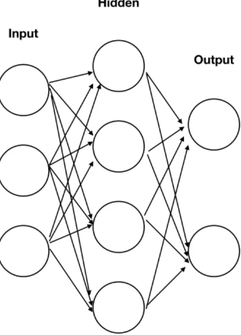
The structure of a neural network can be seen as a directed, weighted graph, as illustrated in Figure 2.1.

Figure 2.1: Illustration of the structure of an ANN.

An artificial neural network consists of a collection of simulated neurons. Each neuron is a node which is connected to other nodes via links. Each link has a weight, which determines the strength of one node’s influence on another [38]. The neurons are typically organized into multiple layers, especially in deep learning. Neurons of one layer connect only to neurons of the immediately preceding and immediately following layers. The layer that receives external data is the input layer. The layer that produces the ultimate result is the output layer. In between them are zero or more hidden layers. Single layered networks are also used. Between two layers, multiple connection patterns are possible. They can be fully connected, with every neuron in one layer connecting to every neuron in the next layer. They can be pooling, where a group of neurons in

(28)

one layer connect to a single neuron in the next layer, thereby reducing the number of neurons in that layer [39]. Neurons with only such connections form a directed acyclic graph and are known as feedforward networks. Alternatively, networks that allow connections between neurons in the same or previous layers are known as recurrent networks. Other than these, there have been many variations being proposed.

2.4 Generative Neural Networks

There is a surge of generative deep neural networks in the recent years. To train a generative model, we first collect a large amount of data in some domain (e.g., think millions of images, sentences, or sounds, etc.) and then train a neural network to generate data like it. The most pop-ular structure nowadays are variational autoencoders (VAE) and generative adversarial networks (GAN).1[40] [41] [42]

The trick is that the neural networks we use as generative models have a number of parameters significantly smaller than the amount of data we train them on, so the models are forced to discover and efficiently internalize the essence of the data in order to generate it.

Generative models have many short-term applications. But in the long run, they hold the po-tential to automatically learn the natural features of a dataset, whether categories or dimensions or something else entirely. This will be an important step towards artificial intelligence.

Currently, all of the different approaches to generative neural networks have their pros and cons. For example, VAEs allow us to perform both learning and efficient Bayesian inference in sophisticated probabilistic graphical models with latent variables. However, their generated samples tend to be slightly blurry. GANs currently generate the sharpest images but they are more difficult to optimize due to unstable training dynamics. All of these problems do not have certain solutions and are very active areas of research now.

(29)

2.5 Entropy and Mutual Information

The entropyH(X)of a discrete random variableX is defined as

H(X)=−Õ

x∈X

p(x)logp(x). (2.12)

It is a function which attempts to characterize the unpredictability of a random variable, both in terms of the number of possible outcomes and its frequency.

The concept of mutual information is intimately linked to that of entropy of a random variable, a fundamental notion in information theory that quantifies the expected amount of information held in a random variable.

Not limited to real-valued random variables and linear dependence like the correlation coeffi-cient, mutual information is more general and determines how different the joint distribution of the pair(X,Y)is to the product of the marginal distributions of X andY. Formally, the definition of mutual information is (again, we only consider both X andY to be discrete)

M I(X;Y)= Õ x∈X Õ y∈Y p(x,y)log p(x,y) p(x)p(y). (2.13) 2.6 Definition of Terminologies

In this coming sections, we will define the terminologies that will be used throughout the whole work.

2.6.1 Task and Objective Function

Definition 2.6.1. A task for a machine learning procedure is the optimization of an objective func-tion.

Commonly-seen tasks are prediction, classification, inference, and variable selection. When defining a task, a corresponding objective function that is based on empirical data should also be

(30)

defined. For example, when one defines “prediction” as the task, there should be a corresponding objective function, such as the sum of squares of the difference between the observed value and the predicted value.

Definition 2.6.2. Objective functions are statistics that we can develop optimization algorithms for.

2.6.2 Feature v.s. Latent Factor/Variable

Features are observable independent variables. Latent factors/variables are unobservable inde-pendent variables that are not present in the dataset. We will refer to the features present in the dataset as the raw feature, and any other transformation of the raw features will be called trans-formed features. Since latent factors/variables are unobservable, they are assumed by the scientists and then learned from data.

Historically, we see there is the trend of learning from raw to transformed features. It starts from feature engineering, the most concrete case, when people hard-code their prior knowledge about the underlying mechanism into the model. For example, in a facial recognition system, we may hard-code features such as the eye color, the face shape and the length of hair into the system. However, in order to expand the scope and applicability of machine learning methods, we actually would like to make learning algorithms to be less dependent on feature engineering [5]. Another rationale for doing this is about data-drivenality – most of the time, we actually have limited knowledge about what good features are, so it would be better for the machine to figure it out by itself from data. More importantly, if we want to make progress towards artificial intelligence, which fundamentally means to understand the environment around, the artificial intelligence agent must have the ability to figure out important underlying explanatory factors hidden in the observed sensory data [5].

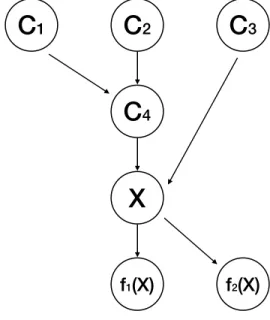
In terms of a data generating process, we define the flow of the data generating factorsCi, the

observable raw features X, and the transformed featuresfi(X), wherei denotes the indexing. The

(31)

observable raw featureX, and the transformed features f₁(X)and f₂(X).

Figure 2.2: A data generating process example.

If we model the data generating process as a sequential procedure, we call everything happened before the raw features as the upstream transformations; similarly, we call everything happened after the raw features as the downstream transformations. So in the previous example, the raw feature is X, the upstream transformations includeC₁toC₄, and the downstream transformations include f₁(X)and f₂(X). The ordering may not impact much in the mathematical modeling stage, but they are essential in adding on interpretability of the model.

In sum, we make the following definitions:

Definition 2.6.3. Transformed features are the downstream transformations of the raw feature. Without seeing the data, neither features or transformed features can be formed.

Definition 2.6.4. Latent Factors/Variables are the upstreams transformations of the raw features. They can be formed without data.

(32)

2.6.3 Feature Selection v.s. Feature Embedding

Similarly, as the development of machine learning in many different applications, different names of similar procedures were generated. We will use the following unifying definition when-ever we mention about these terminologies:

Definition 2.6.5. Feature selection is the process of choosing relevant and useful features for suf-ficing the task.

Definition 2.6.6. Feature embedding is the process of transforming features.

In fact, in this definition, feature selection can be treated as one special case of feature embed-ding, where each feature is transformed into the feature times the corresponding indicator function which indicates the selection decision.

2.6.4 Discriminative Model v.s. Generative Model

Definition 2.6.7. Discriminative models are models that could model the process and give results of either regression (continuous response) or classification (discrete response). They do not neces-sarily reproduce the true data generation process, but is sufficient for the discrimination task. Definition 2.6.8. Generative models are models that try to reproduce the true data generation process. Why do we need generative models? First, they help us understand the data generation process, which may be potentially helpful if we would like to do causal inference or transfer learning. Second, they add on interpretability. And, thirdly, when we don’t have enough data, they can generate more data in for semi-supervised learning purpose.

In some cases, discriminative models can be viewed as a hierarchy embedded inside a genera-tive model. The decision of going for a discriminagenera-tive or a generagenera-tive model should be determined by the interpretability of the corresponding representation and the ultimate task.

(33)

Chapter 3: Sufficient Representation Learning Framework

3.1 Introduction

As introduced earlier, there is the dilemma between inference and prediction. As a statistician, I would like to begin with traditional statistical inference methods, and gradually move towards modern statistical methods that incorporate decision theory, graphical models and Bayesian meth-ods. While each has its own origin and assumptions, practitioners nowadays seem to ignore these important distinctions, which may lead to misuse of the inferences. In this work, we would like to create a unifying framework that connects statistical modeling methods with computationally-inspired black-boxed models such as neural networks. We hope this will provide more insights and correct the practice of statistics into various fields of applications.

One of the major challenges of transporting traditional statistical methods into modern data is the scale of the dataset. At the time while Statistics was emerging, the applicable data wasn’t really big or high-dimensional compared to nowadays data. So even though the model wasn’t exactly “correct”, it may not be too far away from the correct one. However, as more complicated and high-dimensional data emerge, such as genome data and image data, the correctness of model specification has become more important than ever before. So, in this work, we would like to discuss about the interaction between model, representation and optimization for a task – which could probably be omitted when the data was not so complicated, but no longer so once we enter the big data era.

So our first idea of the new learning framework is that, since “all models are wrong” [43], let’s shift our focus on finding models that are interpretable. We call these interpretable models the representation of the data. As machine learning progresses, there are more and more demands into this criteria, especially when we enters the era of artificial intelligence. For example, instead of

(34)

letting a black-boxed algorithm to tell us if the scan photo of a patient’s liver has a tumor, we often feel more comfortable and reliable if the algorithm also tells us why. The consequence of this is that our desirable representations may go before data-fitting, which violates traditional statistical learning principles.

Hence, we would like to suggest that, instead of trying to find the true model (if it exists), we try to find a useful representation within a model that is interpretable and sufficient for a task. Traditionally in model fitting, we have the mindset that there is only one true model, so we have to perform model selection to choose the best one. However, in representation learning, there is no true or false. Representations simply reflect how the scientists interpret the data but they do not need to reflect the true status of the nature. In other words, there can be many different representations for the same data, as long as they are sufficient for their assigned tasks.

3.2 Sufficient Representation – Statistical Desirable Qualities

We are now in the process towards defining what a good representation is. Since the idea of being good may be too subjective, we, instead, identify some desirable properties of an appropriate representation. In Bengio 2014 [5], he discussed about many criteria for a good representation from a computational point of view. Essentially, in machine learning, the performance of the methods is highly dependent on the choice of good features [5]. However, in practice, people choose features based on the performance of the machine learning method. The rationale being that, if the performance of the machine learning method is good, then it must be that the underlying features are good. But is this the right way? Or how about doing it in the opposite way? As discussed previously, in representation learning, we are concerned about the interpretability – if we completely let the performance of a discriminative learning method guide the feature selection or embedding process, the resulting features may not be interpretable. One family of such examples is the L-x penalization methods in linear regressions. While computationally efficient, it can hardly explain the meaning of the results beyond statistical significance.

(35)

optimum representations is not the most important consideration, we may still find representation learning as an important step for modern machine learning problems. For example, if we have a bunch of photos of cats and dogs, and the task is to do classification; while a logistic regression model may well suffice the needs, people still appreciate methods like neural networks that can provide some insights about the representations learned inside the network. Another example is that, in identifying possible cancer patients, decision trees are much preferred than regression methods because of its natural interpretability which provides much more insights for scientists and doctors to look further into the biological meanings of those variables. This is also mentioned in Bengio et al. [5] that the success of machine learning algorithms generally depends on data representation, because different representations can entangle and hide more or less the different explanatory factors of variation behind the data [5]. Although specific domain knowledge can be used to help design representations, learning with generic priors can also be used, and the quest for artificial intelligence is motivating the design of more powerful representation learning algorithms implementing such priors [5].

3.3 Sufficient Representation – Statistical Desirable Qualities

So far, we have discussed some qualitatively desired properties of representation learning. In this section, we would like to propose one statistical criteria, sufficiency, inspired from classical Statistics.

To apply the idea to our proposed partition-based model, the key is to find a partition-based representation such that, conditioned on the representation, the task and the raw features become independent. If that is the case, then we don’t need to worry about the distributions of the raw features, which, in some sense, may help variable selection and dimensional reduction at the same time.

We need to assume that the raw data itself is always sufficient. This guarantees the existence of a sufficient representation for any specific dataset.

(36)

3.4 Definition of Sufficient Representation

Here we would like to define, quantitatively, what a sufficient representation is. The idea is the generalization of sufficient statistics. We have data including raw features X ∈ _Rp, and there may or may not be corresponding labelY. Here we assume Y ∈ _R. Even ifY has more than one dimension, we can deal with one of the dimensions each time, and we assume all of them are independent. We also define a task θ. This θ can be, for example, estimating a parameter, estimating a function, choosing a model, ..., etc. Whether θ is stochastic or not depends on the design and application.

We would also like to define what we mean by “data” – a generalized idea. There are three kinds of data: the observed, the futured, and the unobserved. The observed (or the collected) data is the conventional data. They are the current data that we have already observed their values. We will use subscripts to denote them in order to tell them apart; for example, Xi means the it h

observed data X. The future data is the imaginary data that may exist in the future, but unknown to us at the current moment. The unobserved data can be either in the past, concurrent, or in the future. Since it is never observed, it does not matter when it would happen. A hidden feature also belongs to this category. We will see the importance of these distinctions later.

According to the task, a corresponding objective function fob j(Xi,Yi, θ), or fob j(Xi, θ),

depend-ing on the availability ofY, will be defined. We define the achievement of the task to be obtaining the optimum solution,θ∗, to the objective function. This can be done analytically or computation-ally. In practice, the achievement of the exact solution may not be feasible, but, still, one can try to find a proxy or a subset to the optimum solution. The optimum solution can be written as

θ∗ ₌

argmax_θfob j(Xi,Yi, θ), or (3.1)

θ∗ ₌

argmax_θfob j(Xi, θ). (3.2)

Note that there may or may not be a “true” theoreticalθ. Even if there is one, the optimum solu-tionθ∗from the objective function may or may not equal to the true valueθ. Furthermore, whenθ∗

(37)

is obtained by an optimization algorithm, it becomes a function of the algorithm. This gives prac-titioners more flexibility in designing the objective function and the corresponding optimization algorithm(s).

We define a sufficient representationZto be a function of the data(X,Y), such that the achieve-ment of the task is conditionally independent with the observed data(Xi,Yi), given the

representa-tion. That is,

θ∗ _⊥

⊥ (Xi,Yi)_iN₌₁|Z, or (3.3)

θ∗

⊥⊥ (Xi)iN=1|Z (3.4)

One quick example is to perform MLE on Normally-distributed data – the objective function 3.2, is the Normal likelihood function, and the taskθis to estimate the mean of the Normal distri-bution (assuming the variance is known). According to the theory of MLE, the sufficient statistic is the sample mean. We then interpret (in the representation learning setting) that, the sample mean is the representation for the data in achieving the task of estimating the population mean. In other words, since it is the representation, to estimate the population mean, all we need is the sample mean and we can throw away other information in the raw data. However, the missing piece in classical theory is that the task for MLE learning is for inference, so the results are for inference purpose. If we want more from the results of MLE, such as prediction, it is a wrong use of the model and may lose the interpretability as well.

Next, we would like to propose that, one dedicated objective function should be used for one task at a time. There may not be a universal mathematical benefit of doing this, but this will guar-antee the interpretability of the representation. For example, if our goal is to perform dimension reduction and linear regression, we compare the following two methods: (1) a principle component analysis (PCA) is performed first, and then use the resulting principle components for a linear re-gression, and (2) a linear regression with L-1 penalty (i.e. LASSO). While there are pros and cons for these two methods, we can always say that (1) has a better interpretability than (2), because it

(38)

has a dedicated step for dimension reduction and another one for regression. So we can interpret the results separately; while in (2), the dimension reduction is almost done inside a black-box – it is very hard to interpret the result.

Finally, there is a connection between the objective function and the algorithm that is used to optimize the objective. Even for the same objective function, different optimizing algorithms may yield different solutions. So it is important to specify the pair of “objective function + optimization algorithm” together.

More examples will be present later in this chapter. Before that, we would like to give a general guideline of the procedures that one should follow for performing our proposed representation learning.

3.5 Representation Learning Procedure

In order to implement our proposed sufficient representation learning, we propose the following procedures:

1. Define the task, the corresponding objective function, the optimization algorithm (if no ana-lytical solution), and the desired form of the representation.

2. Define the joint distribution of every variable including the representation, and decompose the likelihood up to the desired level of hierarchy. Choose prior(s) if needed.

3. Find the optimum solution to the objective function and check the sufficiency of the repre-sentation.

4. Use data to perform the algorithm.

(39)

3.6 Notation

In the following sections, more examples will demonstrate how this sufficiency can be achieved in different contexts. Here let us define the notations and terminologies that will be used later in this chapter.

If X ∈ _Rp is a vector that has p dimensions, we will denote each dimension component by X(k), where k means theit h dimension component. In other words, X = (X(1),X(2), ...,X(p)). If X represents a dataset, then we call X(1)the first feature, X(2) the second feature, ..., etc. We will use subscriptions to denote the sample index; for example,X_i(1) means the value of the first featureX(1) for the it h sample. Without special explanations, X is for the independent variables, or features; andY is for the response variables, or labels.

For collected data, we will denote it by (Yi,X

(1) i ,X (2) i , ...,X (p) i ) N i=1 or(X (1) i ,X (2) i , ...,X (p) i ) N i=1,

de-pending on the availability ofY.i is for the index of the (unordered) data values.

3.7 Toy Example

Suppose the true model isY = X(1) + logX(1) +, whereY is the response variable, X(1) is the only true feature, is the error that follows a standard Normal distribution and is independent with X(1). In reality, we collect data(Yi,X

(1) i ,X (2) i ) N i=1, where X

(1) _{is the first feature and}_X(2)_{is the} second feature in the dataset. In other words, there are redundant features in the dataset. However, in practice, we don’t know which features are redundant, nor the true model. How should we model the data?

The common practice that we see is to jump right into some type of regression, hoping that one magical model will do it all.

However, we propose that let us pause for a second and define the task first, since, modeling the data is not done blindly; instead, it should be task-oriented.

Task 1: In our first example, let’s say Task 1 is to predict future Y; that is, to obtain the optimum estimator for futureY, denoted byYˆ. The corresponding objective function is chosen to

(40)

be minimizing the expected square loss E(N1

Í

i(Yi −Yˆ)2), where the predicted future value,Yˆ, is

constructed from the current dataset, andYi’s are the actual future data. We assume that the future

Xare known, so there is no need to be worried about the uncertainty forX. From machine learning theory, we know the bias-variance decomposition:

Assumey = f(x)+ is the true model and fˆis the estimator for f, then we have (3.5)

E( 1 N Õ i (Yi−Yˆ)2)=E(Y −Yˆ)2 (3.6) =E(f(x)+ − f(x))ˆ 2 (3.7) =E()2+E(f(x) −E(f(x)))ˆ 2+E(f(x) −ˆ E(f(x)))ˆ 2 (3.8) =E()2+(f(x) −E(f(x)))ˆ 2+E(f(x) −ˆ E(f(x)))ˆ 2 (3.9)

The minimum of Equation 3.9 is obtained at _E()2, which is the variance ofY. This is often called the irreducible error. One obvious solution is whenYˆ = f(x).

f(x)=argminYˆE( 1 N Õ i (Y_i−Yˆ)2), (3.10)

and it obviously satisfies the sufficiency condition Equation 3.3:

f(X) ⊥⊥ (Y_i,X_i(1),X_i(2))N_i₌

1|Yˆ = f(X), (3.11)

where X without subscriptions is for future values, and Xi and Yi with subscriptions are for

values in the collected data.

However, to obtain the exact true function almost never happens in reality.

Since the task of prediction is actually much less than obtaining the whole true function, the solution becomes much more obtainable and practical, if we are willing to say that, we are not trying to find the true function; instead, we are trying to find a function that can perform the task of prediction as well as the true function. This new function that we construct has our own desired

(41)

properties and is called a representation.

For example, if we use nonparametric regression methods such as a spline and find the esti-mated function fˆspline(x). Let’s assume that, for all x within our interest of prediction, fˆspline(x)=

f(x). Then we also have the sufficiency condition just like Equation 3.11:

f(X) ⊥⊥ (Y_i,X_i(1),X_i(2))_iN₌

1|fˆspline(X), (3.12)

while the functional form of fˆspline(x) can be totally different from the true f(x). We call ˆ

fspline(x)a representation, because it contains our belief of looking at the data through the lens of

the basis functions of the spline, and the results are interpretable using lingos in spline models. In sum, in this example, we used useful representations of the raw features X for the task of predicting futureY. A representation is sufficient if we can fulfill the task using the representation only, instead of using the raw features.

Task 2: In our second example, let’s sayTask 2 is to find influential variables that helps to predictY, then identifying X(1) alone is sufficient for this task, regardless of the functional form. How can we correctly identify X(1)? We propose using our partition-based model and use I-Score as the selection criteria with backward dropping algorithm. In this framework, the partitions in X(1) is sufficient for fulfilling this task, and the corresponding representation is each local mean of Y inside the partitions. More detailed discussion will be present in Chapter 4.

Identifying influential variables is not a typical task in statistical machine learning. However, it is useful for many modern applications. Take, for example, the transfer learning in the context of modern artificial neural networks. The idea is that, the labelsY of a picture may be “attached” a posteriori, and we would like to be able to switch between different labeling domains. For example, if we have a handful of pictures of cats and dogs, we can label them according to the animals inside the picture, or we can also label them according to colorful or black-and-white picture. In this kind of applications, we need to identify some general-purposed influential variables regardless of the functional form. Since the exact functional form may change, if we switch from one domain to

(42)

another, the general-purposed influential variables are less likely to vary a lot from domain to domain.

3.8 Representation Learning v.s. Generative Model Learning

Now we have defined our proposed representation learning framework, and we would like to compare it with a generative modeling learning framework using the new viewpoints. The purpose of this is to provide one more example for distinguishing our method with other existing methods, as well as to pave the background for Chapter 7, when we will discuss the application in a generative model.

Representation learning and generative model learning are two different problems by nature. As discussed previously, representations are subjective in the sense that they reflect the way the scientists interpret the data; while (generative) models are (mimicking) the true, objective data generating process.

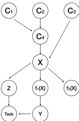
Let’s illustrate the idea using Figure 3.1, which shows the general idea of representation learn-ing. Here we follow the same notations from Figure 2.2, except for addingY, the response variable, Z, the representation, and the task. It is obvious that, in representation learning, we want to learn Z, and all the required information can be taken from X andY, which are observable. However, if we want to learn the generative model, we need to start with all the latent generating factors from C₁toC₄, which may not be viable in practice.

However, as we will develop later, representation learning can actually be beneficial to gen-erative model learning. With the invention of variational autoencoder (VAE), researchers have successfully combined these two kinds of learning together into one architecture. Kingma et al. [40] proposed the idea that learning a generative model can feedback for representation learning. Essentially, we can imagine the task in Figure 3.1 is connected back to the generating factorsC1

to C4. On the flip side, to assess the goodness of the learned representation, one can assess the

goodness of samples generated based on the learned representation.

(43)

Figure 3.1: An illustration of representation learning.

property of the representation. Next, we will shift our focus to how to design an objective function for a specific set of representations, so that the learned representation is as sufficient as possible1. Let’s first do this by reviewing the objectives in the framework of latent variable modeling.

3.8.1 Searching For the Objectives For A Generative Model

Figure 3.2: Latent variable model.

There are many ways of modeling a generative model, one of which is through latent variable

(44)

modeling. In the existing literature, the formulation of latent variable model can be defined through the graphical model as shown in Figure 3.2, where we have data {Xi}_iN₌₁ and latent variable Z, where Xi ∈ Rp and is observable, while Z is not observable and the dimension depends on the

modeling.

The graphical model suggests the joint distribution of the observable Xand the latentZ can be factorized into

p(X,Z)= p(X|Z)p(Z) (3.13)

There are many different objectives for learning these types of model. Particularly, since Z is unobservable, if one marginalizes the latent variable, the typical maximum likelihood method can be applied on the observableX.

p(X)= ∫

p(X|Z)p(Z)dZ (3.14)

Note that since only the data X is observable, if we start from Equation 3.14, there are many different ways of specifying latent variableZ’s. In other words, there is no one unique solution to the latent variableZ’s, even if there truly exists one.

One of the oldest method for learning this kind of model is the expectation-maximization (EM) algorithm. In that setting, we have a pre-defined parameterized distribution of Z, denoted by p(Z). The inference goal is to learn the parameters in the joint distribution of X and Z, denoted by p_θ(X,Z), whereθ is the parameter of interest. The distribution is often assumed to be from an exponential family. Note that the key assumption for this method to work is that the joint distribution pθ(X,Z)has to be fixed. In other words, if we change the distribution on the “prior” p(Z), it cannot change the joint distribution pθ(X,Z). However, how to specify p(Z) remains difficult in practice.

Later, in the variational inference (VI) framework, people claimed that they don’t need to specify the real distributionp(Z); instead, it is only required to specify a proxyq(Z)top(Z|X). In

(45)

our representation learning lingo, thisq(Z)is the representation forp(Z|X). And the goodness of the representation is assessed by the K-L divergence between the proxyq(Z)and the truep(Z|X).

Since

KL(q(Z)||p(Z|X))=−Eq[logp(Z,X) −logq(Z)]+logp(X) (3.15)

⇒logp(X) −_KL(q(Z)||p(Z|X))= _Eq[logp(Z,X) −logq(Z)], (3.16)

minimizingKL(q(Z)||p(Z|X))is equivalent to maximizing the evidence lower bound (ELBO), Eq[logp(Z,X) −logq(Z)]. Furthermore, it is interpreted that, since ELBO is the lower bound of

logp(X), maximizing the ELBO is identical to maximizing the log-likelihood. So it’s the best of both worlds – not only they find a way to perform Bayesian inference in a computationally-efficient fashion, they also preserve the good tradition from classical Statistics (the MLE).

However, there is no free lunch. We would like to point out two cautions for this interpreta-tion. First, for generative model learning, it may be sufficient to use typical MLE as the learning objective, since the purpose of MLE is for inference (under the correct model specification); nev-ertheless, for representation learning, MLE may not suffice to be the optimum objective. Second, in this framework, people often overlook the importance of the populationp(X,Z)being fixed. As mentioned earlier, if we only observe X, there is no way to identify one uniqueZ. Thus resulting non-unique joint distributionp(X,Z). Ifp(X,Z)is not unique, ELBO is not unique, and it is unfair to compare across different models with different lower bounds.

A similar argument was proposed by [fixing the broken ELBO], in which the authors argued that the learning of representations in the context of variational inference should be expanded into a two-dimensional problem by both considering the reconstruction and the distortion rates. In our point of view, this is the same as saying the key population quantity of interest is no longer p(X) alone, but the joint p(X,Z). In the ELBO, the first term gives us the first dimension, which is the reconstruction of observable X, given a chosen Z, and the second term is about choosing one optimumZ.