Examination of machine learning methods for multi-label classification of intellectual property documents

(1)

EXAMINATION OF MACHINE LEARNING METHODS FOR MULTI-LABEL CLASSIFICATION OF INTELLECTUAL PROPERTY DOCUMENTS

BY JOHN W. HALL

THESIS

Submitted in partial fulfillment of the requirements for the degree of Master of Arts in Linguistics

in the Graduate College of the

University of Illinois at Urbana-Champaign, 2017

Urbana, Illinois Advisor:

(2)

ii

ABSTRACT

This thesis explores the performance of a variety of machine learning techniques for the task of multi-label document classification applied to a corpus of United States patent grants. The rapidly rising number of patent applications in the past several decades has led to a rising need for enhanced automatic patent processing tools. The task of automated document classification in particular has been targeted as an important point of research. However, the development of adequate tools has been limited in part by the esoteric writing style particular to intellectual property and the overlapping categorizations of the branched hierarchical classification system employed by the CPC. A patent document corpus offers a large, publicly available training set consisting of both structured and unstructured data. The application of machine learning techniques to this corpus may help relieve the increasing need for highly trained human classifiers. The contributions of the present work are 2-fold. First, the present work constructed a patent document corpus by gathering 4500 patent documents from years 2015 and 2014 and compiling relevant structured and textual data relevant to an automated classification task. Second, it offers an examination of five different machine learning techniques as automated classifiers for patent documents by section. Test trials under different preprocessing conditions utilizing principal component analysis and word selection were applied in training supervised learning classifiers. It was found that principal component analysis of the patent documents without further feature selection yielded the greatest performance for all machine learning models. This approach also revealed an effect of dataset size where increasing the size of the training set increased the overall performance of Decision Tree, Support Vector Machine, Logistic Regression, and Neural Net models. It was further found that some classifiers trained on data not subject to principal component analysis showed decreasing performance metrics with increasing data sizes.

(3)

iii

Chapter 1: Background

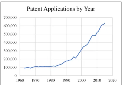
In the past twenty years, the number of applications in the United States for patents has increased dramatically, rising from 220,000 applications in 1996 to 630,000 2015 (U.S. Patent Statistics Chart Calendar Years 1963 - 2015, 2017). The number of examiners employed by the United States Patent and Trademark Office (USPTO) has similarly increased from 2,000 to 8,000 examiners in the same time frame in order to cope with the rising demands on the intellectual property (IP) field. This rapid growth of patent documents has led to a rising call for sophisticated patent analysis tools, tools which forecast future technological trends and identify technological hotspots, and tools which detect patent infringement. However, the preponderance of technical jargon and opaque legal terminology particular to IP documentation, along with terminology changes and development of new technological subfields, necessitates the employment of highly trained professionals, making the process of patent examination slow and expensive.

Figure 1 Number of submitted patent applications by year. Data from USPTO.gov

Much research has been conducted into the automation of the examination of IP [15, 16]. However, its rapidly increasing volume and infamously peculiar writing style, especially of claim language, has presented challenges for automated tools (Larkey, 1998). One task in particular,

0 100,000 200,000 300,000 400,000 500,000 600,000 700,000 1960 1970 1980 1990 2000 2010 2020

(5)

2 | P a g e

document classification, will be discussed as a prime target for automation research. Several machine learning approaches in particular will be examined for their usefulness in the classification task. These approaches will include simple conventional approaches such as Naïve Bayes learning and decision tree learning, as well as more complex and computationally demanding approaches utilizing support vector machines and artificial neural networks.

The present research will examine the effectiveness of each of these machine learning techniques for document classification at five different levels of IP classification. In order to elucidate the nature of the task, background will be provided on document classification as a task in general and on the nature of patent documents and the challenges they present to document classification. The basic foundations of several machine learning approaches will then be discussed, including their relevance to the classification of IP literature.

In this chapter, relevant aspects of IP literature and machine learning are discussed in turn. Discussion of IP will include a description of patent documents, the Cooperative Patent Classification system, and issues presented in automation of patent examining. Discussion of machine learning will include the tasks of document classification, multi-label classification, and dimensionality reduction, as well as appropriate criteria of evaluation for such tasks.

1.1 Patent Documents

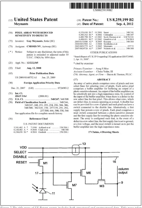
In the United States and internationally, patents have a regular format consisting of a combination of structured and unstructured information. The title page of a given patent grant contains numerous instances of structured data, including the filing number, application date, classification number, etc… However, the bulk of the data contained in a patent document comprises unstructured, textual data contained in the title, abstract, detailed description of the

(6)

3 | P a g e

Figure 2 The title page of US Patent grants includes both structured and unstructured data. Title page taken from US Patent 8,259,199

(7)

4 | P a g e

invention, and the claims. Any analysis or task conducted on such a document must be focused on these sections.

Structured Data Unstructured Data - Publication Number - Title

- Classification Number(s) - Abstract

- Application Number - Background of the Invention - Filing Date - Summary of the Invention

- References Cited - Brief Description of the Drawings - Inventor/Assignee Information - Description of Preferred Embodiments

- Claims

A completed patent grant generally also contains detailed drawings and figures. Such drawings also represent a rich source of information included in standard patent grants. While a full discussion of image recognition is beyond the scope of the present work, these figures represent another potential direction for research in classification and information retrieval tasks.

The detailed description of the document generally comprises the longest section with most information, detailing the structure and function of the invention and generally containing domain-specific terminology, both from the IP domain and the technical domain of the invention. The claims section delineates the legal protections granted to the inventor. While the primary body of a patent contains detailed information on the nature and use of the invention, the claims section spells out the exact legal protections an inventor has secured with the patent grant. The use of legal terminology and the need for very specific language makes claims notoriously opaque and complex in style and structure. Due to legal restrictions on the nature of claims, every claim must consist of a single sentence, sometimes leading to a claim sentence spanning multiple pages in a given document. These sentences often feature “chain expressions” in which one concept is defined, followed by another that further explains an aspect of the previous definition, and so on. This legal quirk thereby leads to the coercion of multiple sentences into one. A prototypical independent claim exemplifying claim structure is reproduced from U.S. Patent 7,222,078 below:

(8)

5 | P a g e

What is claimed is: 1. A system comprising:

units of a commodity that can be used by respective users in different locations, a user interface, which is part of each of the units

of the commodity, configured to provide a medium for two-way local interaction between one of the users and the corresponding unit of the commodity, and further configured to elicit, from a user, information about the user’s perception of the commodity,

a communication element associated with each of the units of the commodity capable of carrying results of the two-way local interaction from each of the units of the commodity to a central location, and a component capable of managing the interactions

of the users in different locations and collecting the results of the interactions at the central location.

Figure 3 The first independent claim of US Patent 7,222,078 displays the single sentence structure typical of intellectual property claims.

1.2 Cooperative Patent Classification

The primary schema used in patent classification in North America and Europe is the Cooperative Patent Classification (CPC). Patent grants and pre-grant publications of patent applications are assigned at least one classification term indicating the subject of application/grant. Additional classification terms may be added to provide further detail on the nature of the invention.

The CPC is hierarchical in nature, featuring five discrete levels denoting increasingly narrow categorization of an application. These levels include Section, Class, Subclass, Group, and

Main group/subgroup. For the fifth level of classification, a tag of “00” indicates classification

(9)

6 | P a g e

group subsumes subgroups classified beneath it, so that a tag of “00” may be said to terminate classification at the fourth level of the CPC hierarchy. The structure of an example classification is denoted for A01B33/00.

Sample classification breakdown for A01B33/00 - Section: letter symbol (A)

- Class: 2-digit number (01)

- Subclass: letter symbol (B)

- Group: 3 digit number (33)

- Main group/ 2+ digits

subgroup:

(00) Figure 4 The CPC system breakdown of a sample classification.

Different nodes within the CPC reflect divisions by scientific/technological field to best categorize inventions into appropriate fields. The topmost level of the CPC hierarchy includes sections for the broadest categories such as “A: Human Necessities”, “F: Mechanical Engineering”, etc… A patent application is assigned a classification at the most detailed level of the hierarchy which is applicable to the invention. However, the invention may be assigned multiple labels to better express the subject of the invention. For example, a jointed surgical tool with an articulating wrist may be assigned into subclass “A61B – Diagnosis; surgery; identification” to reflect its status as a surgical apparatus, as well as “F16D – Couplings for transmitting rotation; clutches; brakes” to further reflect its mechanical aspects. Such an overlapping classification is vital for the process of patent examination since literature from parallel fields often determines the allowance or rejection of an application.

A patent application is assigned a classification at the most detailed level of the hierarchy which is applicable to the invention and as many classification as is necessary to express the scope of the invention. This generates a classification system which is simultaneously fine-grained in specificity and adaptable to the overlapping scope of rising technologies. The CPC itself is an

(10)

7 | P a g e

adaptation of the International Patent Classification (IPC) system which added a number of features and classification nodes, including a ninth section (Y); this section is used to tag technologies spanning multiple sections of the CPC.

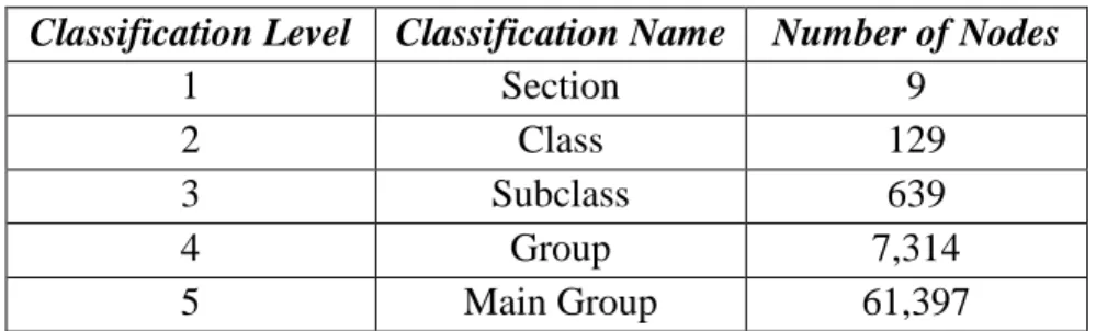
Classification Level Classification Name Number of Nodes

1 Section 9

2 Class 129

3 Subclass 639

4 Group 7,314

5 Main Group 61,397

Table 1 Summary of the CPC levels by number of nodes.

Section Contents

A Human Necessities B Operations and Transport C Chemistry and Metallurgy

D Textiles

E Fixed Constructions F Mechanical Engineering

G Physics

H Electricity

Y Emerging Cross-Sectional Technologies

Table 2 The classification subjects of the nine sections of the CPC.

1.3 Automated Patent Classification

The two primary qualities of IP literature obstructing classification are 1) the relative complexity of lexicon and writing style and 2) the vast quantity of both incoming patent applications and existing published documents (Larkey, 1998).

The first difficulty is tied to the interdisciplinary nature of patent content. IP shows a characteristic combination of highly detailed technical terms and exceptionally broad, ambiguous phrasing. This combination often makes patents less accessible to the lay public and makes the

(11)

8 | P a g e

formulation of adequate search queries challenging. Previous research by Magdy et al. (Magdy, Leveling, & Jones, 2009) has shown cases in which 12% of the documents relevant to a queried topic (as judged by an examiner’s citations) did not share key words in common with that topic. The disjoint lexicons of two such documents stem from the nature of IP documents; patents often contains technological terms specific to a respective field as well as legal terminology which denotes the scope of protection granted to the claimed invention. As discussed above, this scope may overlap different technological fields, such that terminology from two scientific fields are contained in a single document or terms generally used within the scope of one field are instead applied to another. The converse situation also exists, in which two very similar technologies are described in distinct terms.

Moreover, the terminology used in patent literature is notoriously ambiguous and inscrutable in part due to the patent examination process. Examination generally involves a prolonged series of volleys between the applicant and examiner in which the applicant vies for the broadest legal protection possible while the examiner attempts to delineate the application’s legal claims as specifically as possible. This competition between vague and exact phrasing using both technical and legal jargon is further conducted under archaic legal constraints. Patent claims, as discussed above, are required to comprise a single sentence regardless of the complexity of the claim, usually leading to a single, convoluted run-on sentence detailing every feature of the claimed invention. These verbose, esoteric descriptions often make the extraction of useful features difficult for automated tools.

Different approaches have been taken to circumvent these issues in patent classification and retrieval tasks. (Larkey, 1998) constructs document representations for a patent retrieval task using key words which appear at least twice in a patent to produce a candidate vector component.

(12)

9 | P a g e

Key words were additionally weighted according to the document section and number of occurrences per section. However, (Magdy, Leveling, & Jones, 2009) found in a similar task that’ relying on too few words by preprocessing removal of certain sections or low frequency words depressed results in the IR task. The tradeoff is noted that using the full document text with minor preprocessing (such as stop word removal) produced greater results, although with much higher processing times. (Larkey, 1998) further noted that they had not found that the addition of phrases produced superior results to the use of single terms.

Considering these challenges, machinery which will automate sorting of patents into the CPC must overcome at least these challenges:

- Extract usable features from unstructured text

- Recognize linguistic/textual features despite non-standard structures - Have a means to handle or ignore features which are ambiguous

- Recognize overlap of classes despite a lack of overlap of certain features

In addition to these challenges, the accelerating rate at which patent applications are submitted presents a prohibitively large volume of work given that manual classification requires highly skilled human laborers. Analysis of this expanding corpus may therefore be an ideal application for techniques in machine learning.

1.4 Machine Learning

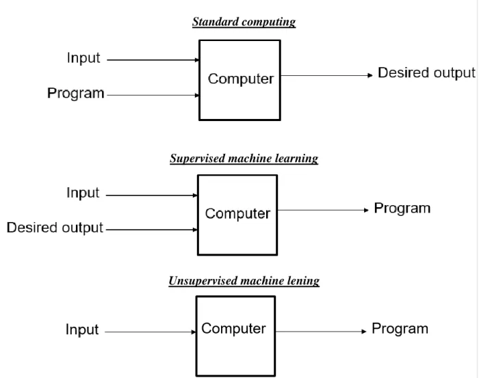
Machine learning comprises the subfield of computer science concerned with designing systems which learn to generate a desired output based on input data (Samuel, 1969). This stands in contrast to standard computer programming in which a system is explicitly programmed to follow a rule-based process to generate its output. In these terms, standard computing may be differentiated from machine learning on the basis of the input and output variables of each case.

(13)

10 | P a g e

Standard “rule-based” computing utilizes an algorithm or series of steps and input to generate a desired output. By comparison, supervised machine learning utilizes a set of labeled training data consisting of input instances paired with their desired output in order to generate a new function; this function may then be applied to further input instances to produce new output.

Unsupervised machine learning functions similarly, but instead infers the function based on unlabeled training data. Supervised and unsupervised methods may be said to differ in the amount of restrictions or patterns provided to the process; supervised learning methods specify explicitly the type/number of expected outputs while unsupervised learning methods determine this information implicitly.

Standard computing

Supervised machine learning

Unsupervised machine lening

(14)

11 | P a g e

Machine learning is data-driven by nature and therefore an ideal subfield for addressing problems which depend on largescale datasets. The vast quantities of unstructured textual data made available by the information age have necessitated tools such as supervised and unsupervised machine learning to complete analyses beyond the scope of human readers. Several specific machine learning techniques are discussed in the present work. However, two overarching tasks are of relevance in the application of these techniques: document classification and dimensionality reduction.

1.5 Document Classification

Document classification is the well-studied problem in information science of how to assign a given sample document or text to a corresponding class. Such documents may be classified according to a variety of features to serve a number of purposes. Document classification has proved important in recent years as a basic form of spam filtering but has numerous applications in identifying the language, authorship, or subject of a given text. Beyond more conventional linguistic identifications, research has demonstrated the vital role machine learning plays in tasks of industry, business, and science which may be decomposed to classification decisions. Applications include medical diagnosis, bankruptcy prediction, and finished product inspection (Baxt, 1990) (Altman, Marco, & Varetto, 1994) (Lampinen, Smolander, & Korhonen, 1998).

While many classifiers work as binary classifiers (i.e., spam vs not spam), a more general case may be described for the multi-class classifier. A basic outline of multi-class document classification models the process as having two inputs, a document d and a fixed set of classes C = {c1, c2, …, cj} (Jurafsky & Martin, 2014). The classification process should successfully output

(15)

12 | P a g e

number of documents made available in the digital age, document classification functions developed by machine learning can be implemented. A machine learning algorithm for document classification is similar to the basic outline but instead generates a function γ which takes documents d as input and outputs their most likely class c.

For the purposes of text document classification, a primary feature extracted from an example document is its word frequencies (Koster, Seutter, & Beney, 2003) (Krier & Zacca, 2002) (Larkey, 1998), where each document is represented by a vector consisting of the word frequencies calculated for that document. The simplest implementations utilize the “bag-of-words” (BOW) approach in which a simple frequency count is obtained (Jurafsky & Martin, 2014). This approach has the advantages of being simple, fast, and computationally inexpensive . However, a common criticism of BOW feature-extraction is that very little linguistic information is retained in comparison to n-gram or dependency parsing approaches which retain more information with regards to word order or relations (Lewis, 1998). Furthermore, it is generally necessary for every document vector to contain a value for each word present in the classification domain, leading to sparsity problem in which every vector contains a high number of zeros in their word frequencies (Dhillon & Modha, 2001).

1.6 Multi-label Classification (MLC)

Multi-label classification (MLC) is a variant on classification problems where a given instance may have multiple output classes. As opposed to standard classification problems (i.e., grouping a given email as either spam or legitimate, but never both), MLC attempts to assign all relevant categories to a single instance (Tsoumakas & Katakis, 2009). Applications of this type of classification problem range through a number of real world situations which often display

(16)

13 | P a g e

overlapping categories, such as a patient in a hospital whose symptoms correspond to multiple relevant conditions or a book which belongs to multiple genres.

It is to be noted that multi-class classification and multi-label classification are not synonymous. A multi-class problem involves multiple possible output types, such as classifying an object to have a single color; a multi-label problem involves assigning all relevant output types to that single object, such as classifying it in terms of both color and shape. To reflect this, multi-label problems are occasionally also referred to as multi-output classifications.

Despite this difference, standard classifiers may be adopted to address MLC tasks. Two prevailing paradigms exist for MLC: algorithm adaptation and problem transformation.

Algorithm adaptation seeks to alter standard classifier techniques used in binary and multi-class multi-classification to directly perform MLC. In this schema, MLC is handled as a single, holistic problem. Such machine learning methods as k-nearest neighbors, decision trees, and neural networks have adapted to address MLC in this way.

Problem transformation methods conversely alter the classification problem into a series of simpler classification problems rather than alter the classification algorithm itself. Two possible tactics may be employed in such a transformation which differ in which aspect of the problem is transformed. In the label powerset transformation, the number of labels is expanded to encompass all possible combinations which may be assigned to an instance. For example, in a training set which has three potential labels “A”, “B”, and “C”, a problem transformation approach to MLC would extend these labels to a complete matrix showing possible overlaps of these three labels such as “A&B”, A&C”, “B&C”, etc… Instances would then be assigned to a single label accordingly.

(17)

14 | P a g e

Example A B C

1 X X

2 X

3 X X

Table 3 Potential training data for an MLC task containing three instances tagged with a set of three labels.

Example A B C A ∧ B A ∧ C B ∧ C A ∧ B ∧ C

1 X

2 X

3 X

Table 4 The training set of Table 3 transformed according to the label powerset transformation.

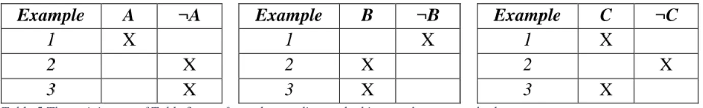
A second problem transformation approach, the binary relevance method, rather than increasing the number of labels, instead increases the number of classifiers. For this approach, a single classifier is trained for each possible label, each of which may be applied in the classification of a single instance. This transformation may be thought of as an extension of a binary classifier applied in a one-vs-all task in which each instance is labeled as either belonging to a single class or not. Thus, as many binary classifiers exist as there are potential labels for the dataset.

Example A ¬A 1 X 2 X 3 X Example B ¬B 1 X 2 X 3 X Example C ¬C 1 X 2 X 3 X

Table 5 The training set of Table 3 transformed according to the binary relevance method.

After the problem transformation is conducted, standard classifier techniques may be applied. In the label powerset method, a single classifier is applied to the transformed data using

(18)

15 | P a g e

the extended set of labels. In the binary relevance method, a one-vs-all classified is trained for each label.

1.7 Evaluation Metrics for Multi-label Classification

Due to the differing nature of MLC and standard classification problems, differing evaluation metrics have been proposed in the literature to capture MLC performance. Because in MLC the predicted and actual values comprise matrices of truth values, it is possible to apply

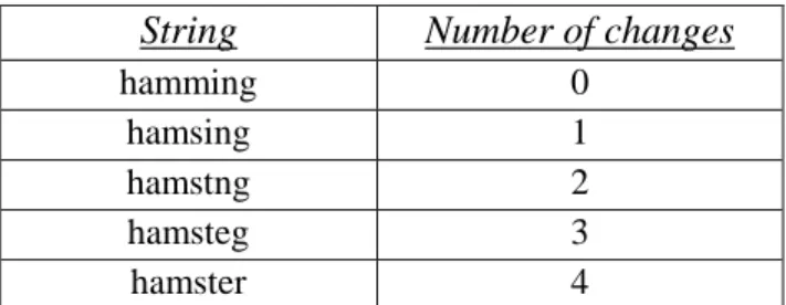
hamming loss as a performance metric (Zhang & Zhou, 2014). Hamming loss is a fractional expression of the Hamming distance is often used to express the “distance” between two arbitrary strings. This distance is measured by the number of steps in a string-editing process, or the number of single alterations required to transform one string into another (Sankoff & Kruskal, 1983). For example, the hamming distance between “hamming” and “hamster” is 4. Hamming loss expresses the error between two strings as a ratio of hamming distance to length of the expected string; in the above example, the hamming loss of producing “hamster” when “hamming” is intended is 0.571.

String Number of changes

hamming 0

hamsing 1

hamstng 2

hamsteg 3

hamster 4

Figure 6 Visual demonstration of the hamming distance between the strings "hamming" and "hamster"

In addition to hamming loss, more standard evaluation metrics may be adapted for use in MLC including precision, recall, and f-measure (Tsoumakas & Katakis, 2009). Precision, or positive predictive value is essentially a measure of what fraction of output classifications have

(19)

16 | P a g e

been made correctly. Recall, or sensitivity, reports the ratio of correct classifications made to the number of classifications that should have bene made. Both values may also be expressed in terms of true positives (tp), false positives (fp), and false negatives (fn).

Because precision and recall alone express different measures of performance, it is possible for a classification system to return high precision with low recall, or vice-versa. To provide a more holistic measure, the f-measure is often computed by taking the harmonic mean of precision and recall.

Figure 7 Precision and recall quantify the false positive and false negative rates of results, providing holistic measures of performance.

Precision, recall, and f-measure are applied straightforwardly to binary classification problems, but may also be extended to MLC. Two schemes, micro-averaging and macro-averaging, are used to accomplish this (Zhang & Zhou, 2014). In micro-averaging classification results, each predicted label instance (positive or negative) across all classes is treated as an individual data point. The appropriate evaluation metrics (i.e., precision and recall) are calculated using each instance to generate an overall score. Macro-averaging instead calculates these metrics by class, generating a discrete precision and recall for each category of label and then averaging these values to determine overall metrics.

(20)

17 | P a g e

In practice, the distinction between micro- and macro-averaging becomes clear if a dataset is unbalanced in terms of labels. Micro-averaging treats each instance from every class as a single instance in the overall class; as a result, classes with large volumes tend to dominate the smaller classes in averaging. So, the micro-averaged precision will closely reflect the precision of the largest classes but not necessarily those of the smaller. Because it assigns equal weight to each class, macro-averaging can be used to provide a clearer idea of performance when data is non-uniform across different labels.

1.8 Dimensionality Reduction

A final consideration in document classification is a practical one and pertains to the dimensionality of the input space. Feature selection refers to the delineation of the subset of predictors for use in model construction; in classification of text documents, features often correspond to textual information (such as a BOW feature vector).

In a large corpus of text documents, the number of distinct words which occur at least once in the corpus may extend into the thousands. This necessitates a very large feature space for the training of a text classification model, where the dimensionality of the input vector is equal the number of words which occur at least once in the entire corpus. High-dimensional training spaces do not theoretically preclude the functionality of classification models; however, in practice overly high dimensionality can prohibitively increase the training time of a model analyzing a large corpus.

Dimensionality reduction is a process of feature extraction used to transform data in high-dimensional space into fewer dimensions. Ideally, this high-dimensionality reduction occurs in such a

(21)

18 | P a g e

way as to remove those dimensions which do not account for a significant portion of the variance observed in the dataset while retaining features which are substantially predictive.

(22)

19 | P a g e

Chapter 2: Machine Learning Methodologies

A significant amount of research has been conducted on the usefulness of machine learning approaches for the task of document classification generally. The foundational nature of several machine learning approaches is discussed, including principal component analysis, k-means clustering, Naïve Bayes learning, decision tree learning, support vector machines, logistic regression, and artificial neural networks.

2.1 Principal Component Analysis

Principal Component Analysis (PCA) is a statistical method for analyzing patterns present in data by performing covariance analysis between factors in the data set (Pearson, 1901). As a statistical method, PCA is commonly applied tool of dimensionality reduction performed on high-dimensionality datasets before implementation in further tasks. PCA functions by identifying dimensions of high variability and reducing the data to a series of “components” with minimal loss of information.

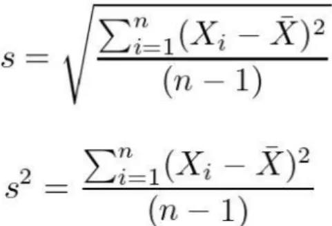
Several concepts from statistics are informative in the implementation of PCA. It is recalled that the standard deviation (s) and variance (s2) of a dataset represent the spread of the data, calculated by measuring the average distance of the mean to each of the data points in the set:

(23)

20 | P a g e

Figure 8 Standard deviation and variance provide metrics of the spread of a dataset around its mean.

These measures describe aspects of 1-dimensional data; covariance represents an analogous aspect of 2-dimensional data, or the relationship between two different factors in data. The same way variance represents how much data varies from the mean, covariance measures how much data points with 2-dimensions vary from the mean with respect to each other. The covariance of two variables X and Y is calculated:

Figure 9 Covariance captures the spread of data with respect to two factors X and Y

It is noted that the covariance of a variable with respect to itself (i.e., X and X) is equivalent to that variable’s variance. Covariance is always calculated between two variables, so data consisting of multiple dimensions may have multiple covariance values. These values may be represented in a covariance matrix. For example, a dataset with three dimensions (X, Y, and Z) will have 9 possible covariances:

(24)

21 | P a g e

It is further noted that because of the transitive property of multiplication in the definition of covariance, the values cov(x, y) and cov(y, x) are the same.

A final concept instrumental to the understanding of PCA involves eigenvectors. For a given linear transformation, an eigenvector is a non-zero vector that does not change its direction when that linear transformation is applied it. That is, when a linear transformation is applied to an eigenvector, the resulting vector is a multiple of that eigenvector. The value of this multiple is correspondingly called an eigenvalue.

Eigenvectors can only be found for square matrices, but not all square matrices will have eigenvectors; if such an n x n matrix does have eigenvectors, it will always have n such vectors. Crucially, each of these eigenvectors is perpendicular to the others.

In order apply PCA to a given dataset (Shlens, 2003):

- Subtract the mean of each dimension from data points in that dimension (this centers the data around zero)

- Calculate the covariance matrix of the transformed data

- Calculate the eigenvectors/eigenvalues of the covariance matrix

The eigenvector with the highest eigenvalue is known as the principal component of the dataset. This eigenvector will point along the data similarly to a line-of-best-fit and will be the eigenvector that best characterizes the variance in the data. The eigenvector with the second

Figure 10 A covariance matrix demonstrating possible covariance values calculated for three factors x, y, and z.

(25)

22 | P a g e

highest eigenvalue will be perpendicular to the first and will second best characterize the variance in the data, and so on.

In high-dimensional data, it is possible that some eigenvectors have sufficiently high eigenvalues as to account for the majority of the variance in the data. If this is the case, it is possible to use PCA to reduce the data to only the dimensions represented by the highest valued eigenvectors; this reduces the dimensionality of the dataset without serious loss of information.

2.2 k-Means Clustering

k-means clustering is a clustering technique common in data mining. The method attempts to partition observations into a set number of clusters (this number denoted as k) on the basis of the mean of the attributes of each cluster. Data points are assigned to the cluster whose mean is closest in value until clearly delineated groupings emerge.

It is instructive to specify the difference in terminology between classification and clustering. Classification, as detailed above, assigns instances into a predefined set of categories determined before the time of classification. Conversely, clustering is the process of grouping a set of instances to determine whether any relationship between instances exists; in such a case, there may not be predefined categories but observable groupings emerge based on discovered patterns and relationships. In the parlance of machine learning, classification is referred to as supervised learning while clustering constitutes unsupervised learning.

Despite belonging to a field lateral to classification, k-means clustering may still be useful in delineating coarse-grained categories as in the case of a document classification task given that the text of the documents are sufficiently distinct to be resolved by clustering. Clustering in this approach utilizes the following algorithm (Hu, Zhou, Guan, & Hu, 2008):

(26)

23 | P a g e

1) Randomly define k initial clusters and calculate their means;

2) Proceed through the list of items, assigning an item to the cluster whose mean is nearest, recalculate the mean for that cluster which receives the new item and for the cluster losing the item;

3) Repeat Step 2 until no new assignments take place.

k-means clustering provides a fast, robust, and easily-understood approach to document clustering. It is relatively efficient and provides good results when datasets are distinct or well-separated from each other. However, if the datasets are overlapping k-means cannot always resolve the presence of two distinct clusters. It also suffers from an inability to reliably reach a globally optimal solution. Because the k-means algorithm begins with a random initial seed, there is no guarantee that the best clusters will be determined over locally optimal ones based on the initial cluster centroids.

2.3 Naïve Bayes

Naïve Bayes (NB) refers to a simple statistical classifier often cited as the baseline statistical classification method. It has been featured in a number of classification problems and research studies as a simple but nonetheless powerful point of comparison for more complex classification systems (Zhang P. G., 2000). NB classification is “naïve” because of its foundational assumption that features are independent of each other. While this assumption is rarely true for features such as words in a text, NB still shows fair performance in tasks such as document classification.

(27)

24 | P a g e

Where d is an instance of a document and c the instance of a class. Read in prose, this theorem states that the probability that a given document belongs to a certain class is equal to the probability of that same document appearing in a given class, multiplied by the probability of the class and divided by the probability of seeing that document. This logic may seem circular, but it allows for a great simplification of the classification problem; because the task centers on selecting the most probable class for an instance, the most likely class may be modeled as:

Because the probability of the document remains constant for all classes, it does not have mathematical relevance for determining the most probable class. The document itself may be further decomposed into a vector of its features (i.e., its word counts) such that the probability may be further rewritten:

Note that this method may therefore easily employ the BOW assumption. Classification then proceeds as a count of words contained in the relevant documents applied in the final formula. NB, relative to more complex methods, is very fast and has low storage requirements. However, the independence assumption at the core of NB means that this technique shows optimal performance if that assumption holds; NB has been criticized for completely ignoring relevant linguistic features which are lost with the BOW approach. However, NB continues to serve as a dependable baseline in text classification even as alternative techniques are presented to have better accuracy.

(28)

25 | P a g e 2.4 Decision Trees

Decision Tree (DT) learning attempts to implement macroscopic categorization as a series of smaller categorization decisions on the basis of specific features. DT learning has become one of the most widely used methods of inductive inference due to its resistance to noisy data and ability to construct models trained even with missing data (Mitchell, 1997).

DTs classify instances by sorting them through a series of branched nodes; each node considers a particular attribute of that instance, passing it down one branch if that attribute meets a certain condition or the other branch otherwise. Once passed to a subsequent node, the process repeats, testing an attribute of the instance and passing it along until a terminal node is reached reflecting a final classification. As a result, each path from the root node to a terminal node represents a conjunction of attribute tests, each attribute showing a certain value traceable along the path.

Problems tend to be suited to DT when they show certain characteristics. In particular, the target function generally has discrete output values rather than real-valued numerical outputs. In its simplest form, DT learning assigns Boolean classifications (e.g., yes/no) for each tested instance; however, this process is readily extended to learning functions with more than two output values (Mitchell, 1997). This makes a DT model well-suited to the task of automated classification. DT learning is also easily adapted to input instances constituting attribute-value pairs, generally a fixed set of attributes with disjoint possible values. However, as previously noted, the training data may contain instances of errors or missing attribute values as DT learning is generally robust against unknown or noisy data.

(29)

26 | P a g e

The basic DT learning algorithm makes use of a top-down greedy search through the hypothetical space of possible trees. This approach is exemplified by the ID3 algorithm introduced by (Quinlan, Induction of Decision Trees, 1986) and the extended C4.5 (Quinlan, C4.5: Programs for Machine Learning, 1993). Here, the ID3 algorithm is explored as the basis of DT development. The standard algorithm constructs DTs top-down, essentially beginning with the question of which attribute should be tested at the root of the tree. To answer this, each instance attribute is evaluated using a statistical test to determine how well it alone classifies the training examples. Whichever attribute best categorizes the data is selected and used as the root node test. A descendant of this node is then created along each resulting branch, and then the training examples are sorted to the appropriate leaf. At each subsequent node, the process is repeated using the sorted training instances to select the best attribute for testing at each new node.

Note that this constitutes a greedy search in which the algorithm never backtracks to reconsider its earlier choices. Pointedly, this means that the central choice of DT learning is the selection of which test attribute is most useful for classifying the training data. This necessitates a strong quantitative measure to gauge the decision at each developing node. The measure used in ID3 (and many extended algorithms) is a value borrowed from information theory: information gain.

To describe selection by information gain it is illustrative to first give an information theoretical definition of entropy. In a linear classification problem between two arbitrary classes A and B of all examples in a set S, entropy may be defined mathematically:

Entropy(S) = –pA log2(PA) – pB log2(pB)

Where pA is the proportion of examples in S falling into class A, and pB the proportion

(30)

27 | P a g e

class, the entropy is 0; when S contains an equal number of instances of both classes, the entropy is 1. All other cases show an entropy between 0 and 1 (Shannon, 1948).

Using these principles, entropy may therefore be interpreted as the amount of information needed to encode the classification of a member of S. When all members belong to the same class, no information is necessary (since it may be assumed correctly which class any instance belongs to). If an equal number of members of each class exist, there is no statistical likelihood of any one instance belonging to one set over the other so the maximum amount of information is needed to describe the examples of the set (i.e., the categorization of an instance is at its hardest to guess). It may further be noted that this principle is easily extended to cases for which target classification takes on an arbitrary number of possibilities:

Entropy(S) = for i in c: Σ –pilog2(pi)

In the context of DT development, information gain measures an expected reduction in entropy and is the measure employed by ID3 at each node to select the best attribute for a given node test. If categorization by a particular attribute creates a subset with an especially great reduction in entropy (i.e., a high information gain), that attribute represents a good candidate for testing at that point in DT development.

For use in a classification task, DTs presents the advantage of running a complete search through the training data and attribute space during tree growth. Due to the greedy top-down search employed in its basic algorithm, it also places attributes with the highest information gain closest to the root of the tree and selects the shortest tree it encounters over the course of its simple-to-complex search. On the other hand, use of DT learning poses risks with overfitting to training data (Mitchell, 1997). It may be said that a model “overfits” if a model which performs less well on the same training data outperforms using an overall dataset. Because each branch grown in ID3 is

(31)

28 | P a g e

grown to perfectly fit the input data, it may be subject to such overfitting. Modified algorithms avoid this issue by shortening the growing time of the DT or by allowing the DT to overfit the training data, and then post-pruning the tree to a simpler model.

2.5 Support Vector Machines

Support Vector Machines (SVM) are supervised learning models that classify data through the lens of high-dimensional analysis. In this approach, example instances are mapped as points in space on the basis of high-dimensional vectors representing the features extracted from the classified objects. The SVM returns the function best spatially dividing these points into distinct groupings. The nature of this function depends on the space in which it is assigned and is often characterized as a hyperplane. In geometry, a hyperplane is any subspace having one less dimension than its environment: a hyperplane may constitute a dimensionless point dividing data on a 1-dimensional line, a line bisecting points on a 2-dimensional plane, a plane separating objects in 3-dimesional space, and so on.

SVMs as a linear classification tool were introduced by (Cortes & Vapnik, 1995) as a means of generating a hyperplane separating instances in space and orienting this hyperplane in such a way that it is the greatest distance possible from the closest member of both classes. The hyperplane so described may then be defined in terms of a linear function with (ideally) all members of two classes falling on opposite sides of this function. However, SVM methodology can be expanded to handle data that is not fully linearly separable by relaxing the constraints on the model to allow for “misclassified” points according to a linear separation. In such a model, data points on the incorrect side of the margin boundary incur a penalty that increases with the point’s distance from the boundary. This allows for the construction of an SVM which still

(32)

29 | P a g e

optimizes hyperplane orientation by minimizing its distance to data points which are ostensibly positioned on the wrong side of the hyperplane while still fitting the data overall.

While functions dividing points in space are often visualized in small numbers of dimensions, a family of functions known as kernel functions exist which can recast functions into higher dimensionality space, allowing SVM classification utilizing vectors with high numbers of features (such as the complete set of counts of words extracted from a text document). These kernel functions allow the adaptation of SVMs to non-linearly separable data.

However, a major downside to SVMs is their long, inefficient training time. This has limited industry-scale application of SVMs and limited their use with larger training sets. Additionally, extension of the SVM approach to multi-class classification involves reducing a single multiclass problem into a series of binary classification problems, further adding to the necessary training time of the approach.

2.6 Logistic Regression

Regression analysis denotes any statistical process for building a model estimating relationships between one or more independent variables and a dependent variable. Logistic regression models the probability of an event, either binary or categorical in nature, depending on input variables of categorical or numerical value. This model predicts the effects of these variables on the response variable and can classify observations by estimating the probability that said observation belongs in a given category.

The linear regression model uses a normal least square approximation or linear equation as a basis (Peng, Lee, & Ingersoll, 2002) (Fujino & Isozaki, 2008):

(33)

30 | P a g e

Where Y represents the model’s output, a stands for a constant value (the intercept in graphical terms), B and X a multiplier and value for an independent variable, and e an error value. B represents the model’s estimation of the impact of a given independent variable.

While this mathematical approach to a regression model functions well for some data, it has the drawback of outputting infinitely positive values for high independent variable values (and negative outputs for very low ones). This may be inappropriate for certain applications, so logistic regression remedies the issue by transforming a standard regression model to produce outputs between 0 and 1:

The logistic regression model can slower to train than other statistical models such as Naïve Bayes models, but has the advantages of adapting well to categorical data and transparently showing the weighting different factors have on the overall output.

2.7 Artificial Neural Networks

Neural Networks (NN) comprise complex machine learning models analogous to the intertwined network of neurons constituting the brain. In such models, the distinct units of the NN are organized into layers which respond to input by further stimulating or inhibiting a future layer, just as webs of neurons stimulate or inhibit successive neurons in response to stimuli.

At the core of early NNs was the perceptron, a type of artificial neuron first introduced by (Rosenblatt, 1958). The perceptron takes several binary inputs and produces a single binary output. Each input has an associated weighting factor such that the respective inputs contribute different degrees to the expression of the output. This output is determined by whether the weighted sum is

(34)

31 | P a g e

greater or lesser than some threshold value determined by the perceptron’s bias. If the output overcomes this bias, a binary output of 1 is provided; if not, the output is 0.

On the basis of the perceptron as a unit, an overarching NN is constructed with multiple layers each consisting of one or more perceptrons. As a result, the nature of the NN as a whole may be described in terms of the parameters (the weighting values and biases) of the perceptrons. The training of NN-based model, then, depends on the adjusting of these parameters to produce the desirable behavior of the network.

Unfortunately, perceptrons tend to be easily altered by small shifts in weighting values; in fact, a small change in the weights or bias of a single perceptron can cause the output of the perceptron to completely flip, thereby drastically altering the functionality of the deeply interwoven network (Nielsen, 2015). This makes gradually modifying the parameters difficult in practical applications.

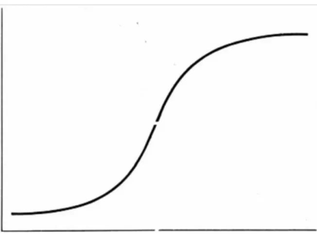
This issue may be overcome by a different type of artificial neuron, the sigmoid neuron. The sigmoid neuron has a series of weighted inputs which produce outputs similarly to the percepton, but these inputs and outputs may take any value between 0 and 1. This is because the functionality of the sigmoid neuron is not binary but rather defined by the sigmoid function:

(35)

32 | P a g e

Figure 11 The sigmoid function produces a characteristic "s-shaped" curve bounded by 0 and 1.

It may be noted that the graphical shape of the sigmoid is reminiscent of a smoothed out binary step function, indicating the mathematical similarity of the functionality of the sigmoid neuron and that of the perceptron. The use of the sigmoid function makes the NN more robust against minor changes in weighting values and biases, allowing for fine-tuning of the network without completely reversing the behavior of neurons in the process.

The architecture of neural networks generally involves a layout consisting of one or more “neurons” which directly receive input values, forming the input layer. The network likewise contains a final layer directly generating the final output of the NN, thus referred to as the output layer. Between these may be any number of layers known as the hidden layers. NNs containing more than one such hidden layer are often called deep neural networks (DNN). A major aspect of NN design consists in determining the arrangement and number of neurons in these different layers, including the number of hidden layers which separate the input and output.

In models thus far described, neurons in the NN generate output from one layer which forms the input of a subsequent layer. Such networks are feedforward NNs, indicating that there is no feedback loop in the network. Conversely, recurrent NNs (rNNs) allow for the possibility of feedback. In such models, neurons fire for a limited duration before going silent. Other neurons

(36)

33 | P a g e

fed by the output of these quiescent neurons themselves fire for a limited time, thereby stimulating adjacent neurons before becoming quiet as well. This results in a steady cascading process which allows the output of neurons to provide feedback to previous layers after a set duration of time rather than instantaneously, thereby ensuring that a neuron does not recursively affect its own output.

The most widely used algorithm for adjusting NN parameters is called the back-propagation of error. In this method, the initial configuration of the NN is arbitrarily set; the result of presenting training data to the NN likely then produces incorrect output. The errors for all inputs patterns are propagated backwards through the network, from output layer back towards the input later. As back-propagation proceeds, the parameters are adjusted to minimize the residual error between the actual and desired outputs of the training data.

Due to their complexity in design and training, NNs essentially function as black boxes; apart from defining the general architecture of the network and seeding the random starting weights, the user plays little to no direct role in the creation of the NN. These nets also tend to be slow to train on serial systems as a result of their highly parallel structure and tend to be inefficient to build on anything but truly parallel systems (Nielsen, 2015).

(37)

34 | P a g e

Chapter 3: Maching Learning in Classification

In light of the large (and growing) number of learning techniques available, researchers are also interested in exploring which methods of classification can most improve classification accuracy. (Fall, Torcsvari, Benzineb, & Karetka, 2003) compared the performance of several classification techniques in the categorization of patent documents, including NB and SVM techniques. Other approaches explore hybrid categorization systems functioning in multiple steps. (Chen & Chang, 2012) research the viability of a three-phase classification system: first, an SVM classifier is trained to categorize patent documents to their first subclass; next, a separately trained SVM classifier organizes the patents into the bottom level of the IPC; a final k-nearest-neighbors classifier then assigns each document its classification code. This multi-phase approach may merit further exploration in a variety of machine learning techniques with different levels of textual pre-processing.

The state of the present literature with respect to different aspects of classification of text documents generally and IP literature specifically is herein discussed, including discussions of the tasks of multi-label classification, feature selection, and patent classification.

3.1 Automated Patent Classification

The applicability of machine learning techniques to document classification in general and patent classification in particular is a burgeoning field of research (Krier & Zacca, 2002) (Larkey, 1998) (Magdy, Leveling, & Jones, 2009). As a data set, IP documents exhibit a number of aspects and challenges to straightforward classification. (Larkey, 1998) notes at the time of publication that the working data comprised 5 million documents and 100-200 gigabytes of text. While the

(38)

35 | P a g e

authors note that the corpus further contains 4-5 terabytes of image data, the retrieval/classification of images is an ongoing line of research not further discussed in the present account.

Despite the great amount of data available for building automated classifiers, issues exist in applying this data in training. It is commonly the case that two patent documents from the same classification category, or two documents deemed by human patent examiner to refer to similar content, do not contain many words in common. Research by (Magdy, Leveling, & Jones, 2009) into patent information retrieval found cases in which documents relevant to a queried topic contained words in common with that topic only 12% of the time. (Larkey, 1998) cites one possible explanation for these discrepancies as intrinsic to the patent examining process, in which inventors strive to demonstrate novelty in their work:

As in many other real-world classification and retrieval problems, there is a severe vocabulary mismatch problem. Patents or patent applications about similar inventions can contain very different terminology. Unlike some other domains, inventors sometimes do this intentionally so their invention will seem more innovative.

(Larkey, 1998)

(Fall, Benzineb, Guyot, Torcsvari, & Fievet, 2003) further note the ramifications of the lexical issues of IP for in the International Patent Classificaiton (IPC) system, the precursor to the CPC: “The terms used in patents are quite unlike those in other documents…Many vague or general terms are often used in order to avoid narrowing the scope of the invention.” (Fall, Benzineb, Guyot, Torcsvari, & Fievet, 2003) cites a particular example of the effects this practice can have, noting that it is common in the pharmaceutical sphere to recite all possible therapeutic uses for a given compound. This adds a great deal of data to a given document without necessarily contributing the spirit and scope of the invention which is used in determining its classification.

(39)

36 | P a g e

The nature of different classes also entails differences in vocabulary diversities. Classification C07: “Organic Chemistry” for example makes by far the largest contribution given the numerous long DNA sequences it contains. The vocabulary diversity is likely indirectly compounded by a legal restriction on patent applications: each application is only granted if the invention is novel or a non-obvious adaptation of previous technologies. As a result, patents are necessarily all different at the semantic level; if semantically identical, two patent applications could not simultaneously be granted.

IP literature also do not show a uniform distribution between different classes, instead favoring a somewhat Zipfian distribution. A large number of classes contain roughly similar document classes, but (Fall, Torcsvari, Benzineb, & Karetka, 2003) list certain class/subclass categories such as A61: “Medical or Veterinary Science, Hygiene”, H04: “Electric Communication Technique”, G06: “Computing, Calculating, Counting” and C12: “Biochemistry” as receiving a disproportionately large number of applications.

Further compounding the complication of constructing an automatic classifier for patent documents are several rules and norms dictating the placement of each document into its corresponding label(s). (Fall, Benzineb, Guyot, Torcsvari, & Fievet, 2003) note in particular one rule for selecting the primary classification of a given application which holds that the second of two feasible categories should be selected if two are found to concord with the subject of the patent application. Additional rules applicable to secondary categorizations complicate label-assignment by imposing certain requirements and restrictions for different categories. The authors describe one such rule related to secondary classification assignment:

A majority of patents do not have a single main IPC symbol, but are also associated with a set of secondary classifications…In some parts of the IPC, it is obligatory to assign more than one category to a patent document if the patent document meets

(40)

37 | P a g e certain conditions. For example, in subclass C12N: “the therapeutic activity of single-cell proteins or enzymes” is also classified in subclass A61P.

(Fall, Benzineb, Guyot, Torcsvari, & Fievet, 2003)

3.2 Multi-label Classification in Text Categorization

Existing studies in the literature demonstrate the differences in training time and performance of distinct classifiers on different corpora. Numerous such studies compare the effectiveness of different learning algorithms for text categorization in terms of learning speed, real-time classification speed, and classification accuracy, often utilizing the easily trained and test Naïve Bayes model as a baseline (Dumais, Heckerman, & Shami, 1998), (Zhang P. G., 2000) (Lewis, 1998).

Due to the multi-output nature of the patent classification task, implementation of such machine learning methods must be adjusted to handle multi-label training and testing data. (Tsoumakas & Katakis, 2009) provide a theoretical review of implementation of several methodologies under both major multi-label classification paradigms, as well as more directly examine the efficacy of different approaches under the problem transformation paradigm. The review observes that several algorithm adaptation methods actually directly reflect the problem transformation approaches. With regards to the ML-kNN algorithm, an adaptation of the kNN learning algorithm for multi-label data, it is observed that the method follows the paradigm of the binary relevance method. Further describing the adaptation of the C4.5 decision tree algorithm for multi-label data, the authors note the relationship between the two paradigms in the algorithm’s implementation:

Although these two algorithms are adaptations of a specific learning approach, we notice that at their core, they actually use a problem transformation.

(41)

38 | P a g e

The experimental examination entailed training several multi-label classification models under three different problem transformation approaches. Interestingly, the authors report the best performances in conjunction with the label powerset transformation, despite this approach being less popular in the literature than the binary relevance method.

This disparity in popularity of the two problem transformation approaches may lie in their relative training time and efficiency. One disadvantage of the label powerset transformation approach to multi-label classification is its increased training time. Given a transformation involving N distinct classes, this approach must fit (N2 _–_N_{)/2 distinct classifiers. Because of this}

O(N2) complexity, this problem transformation approach tends to be slower than the binary relevance approach (Pedrogsa, et al., 2011).

Different classifier models have been implemented to overcome the obstacles offered by the automated patent classification task. (Larkey, 1998) remarks that kNN approaches may scale up well from small to large data sets, making them suitable for incremental analyses of performance while scaling up the size of the training data. However, Bayesian classifiers should a greater ability to distinguish closely related subclasses, so that the chosen approach is a combination two-phase classifier. The approach first uses a kNN classifier to categorize input data, followed by a Naïve Bayes classifier to further refine selections made during the first phase. However, previous classification work by (Fall, Torcsvari, Benzineb, & Karetka, 2003) indicates that SVM classifiers may outperform other methods, particularly at the subclass level. However, their experimental results further indicate that precisions for all methods at the subclass level were below those for the class level, possibly indicating the increased difficulty of accurate classification at the lower nodes of the CPC hierarchy.

(42)

39 | P a g e 3.3 Feature Selection for Classification

Although a number of sophisticated document representation techniques exist, the simple and natural BOW representation remains popular. Prior research has cited the best known multi-class multi-classification results for the Reutuers-21578 data set as obtained using BOW approaches (Dumais, Heckerman, & Shami, 1998). As previously noted, the complete library of granted US patents is a vast corpus exhibiting a rich vocabulary diversity. As a result, an automated classifier implementing a BOW approach for the raw text of the patent corpus would have to be capable of handling a large number of documents with a high-dimension input space. To improve the efficiency of such a classifier, numerous attempts have been made to reduce the dimensionality of the input space with appropriate feature selection.

(Dumais, Heckerman, & Shami, 1998) utilize a BOW approach in text categorization; however, their approach conducts feature selection on the basis of word frequency and mutual information. The 300 features with the greatest mutual information were selected for training an SVM classifier, while the 50 greatest features were selected for other classifier models. The selected features were treated as binary (word present or word absent) rather than counts; although non-binary feature classifications were attempted, the authors did not note improvement over binary approaches and did not pursue this technique further.

Other more indirect approaches to reduce the number of features include limiting the number of words which are represented in each document. For example, work by (Larkey, 1998) suggests successful classification of patent documents in particular may be accomplished using only select sections of the overall document. Work (Fall, Torcsvari, Benzineb, & Karetka, 2003) followed this, finding that for each of a variety of tested machine learning algorithms, the most

Examination of machine learning methods for multi-label classification of intellectual property documents

ABSTRACT

TABLE OF CONTENTS

Chapter 1: Background

Chapter 2: Machine Learning Methodologies

Chapter 3: Maching Learning in Classification