Structured Deep Learning for Fine-grained Visual Classification

(1)

STRUCTURED DEEP LEARNING FOR FINE-GRAINED VISUAL

CLASSIFICATION

Master of Science Thesis

Examiners: Prof. Joni-Kristian Kämäräinen Dr. Ke Chen

Examiners and topic approved in the Computing and Elec-trical Engineering Faculty Council meeting on 8th June 2016

(2)

ACKNOWLEDGEMENTS

I finished this Master thesis on a red comfortable chair in Computer Vision Lab in the Department of Signal Processing at Tampere University of Technology. Thanks to this lab - Vision Group of TUT.

This thesis would not be completed without the support of many persons. Foremost in my mind, I want to thanks my supervisor Professor Joni-Kristian Kämäräinen and my advisor Doctor Ke Chen. The former offered me perfect balance of necessary constraint and freedom, while the latter person showed me the pros and cons of different decisions I made, fractional but important. Joni, you helped me preparing and checking my submis-sion to conference again and again, and your good writing style impressed me. Owning to you, I felt that I get addicted to deep learning. Ke Chen, I admired your decent taste of papers and drafts, and these selective materials helped me understand the deep learning community.

I also want to thank my many colleagues in same lab (not in order) Fatemeh Shockrol-lahdi, Nataliya Strokina, Ekaterina Riabchenko, Junsheng Fu, Antti Hietanen , Yuan Liu and Dan Yang.

(3)

TAMPERE UNIVERSITY OF TECHNOLOGY Master’s Degree Program in Information Technology

YANLIN QIAN: Structured Deep Learning for Fine-grained Visual Classification Master of Science Thesis, 48 pages, 0 Appendix pages

September 2016

Major: Data Engineering

Examiners: Prof. Joni-Kristian Kämäräinen, Dr. Ke Chen

Keywords: deep neural networks, convolutional neural network, recursive neural network, computer vision, machine learning

We propose a structured decision making approach using privileged information that im-proves the popular deep convolutional neural network (DCNN) methodology for visual class detection. This is achieved by discovering and exploiting additional privileged -information available only during training. We instantiate learning with privileged infor-mation by defining “latent sub-tasks” that indirectly contribute to the main task – fine-grained visual classification. Specifically, detection of the object location, detection and selection of the object parts or detection of a semantic super-class are examples of la-tent subtasks which we exploit. In the experiments, our framework using deep privileged parts consistently improves the performance of fine-grained classification and our results are comparable to or better than the state-of-the-art methods without requiring expensive human efforts to provide additional annotations on object parts in both training and testing phases, which is thus suitable for scaling to large-scale data owing to its part-annotation-free manner.

(4)

List of Figures

1.1 An example telling whether a classification case belongs to fine-grained classification. . . 1 1.2 We extend the popular DCNN methodology by defining “latent sub-tasks”

which improve the deep fined-grained classification performance. Privi-leged information available during training (e.g., class hierarchy and an-notated bounding boxes or object parts) is used to define the latent sub-tasks. During testing the privileged information is inferred automatically and contributes to the main task via structured decision making. . . 2 2.1 The selected Examples of the OXIIIT Pet Dataset (the top row), the

Caltech-UCSD Birds-200-2011 Dataset (the middle row), and the Columbia Dog Dataset (the bottom row). . . 8 2.2 Samples from ImageNet Dataset . . . 9 2.3 The mathematical model of a single neurone with inputs, activation

func-tion and output. . . 11 2.4 Left: Sigmoid Function, Right: Tanh Function . . . 11 2.5 A MLP with 3 inputs, 3 hidden layers of 3 neurons each layer, and 1

output. . . 12 2.6 RNN architecture unfolded in three time steps. . . 14 2.7 A LSTM network consisted of five computational units. Thetanhrefers

to point-wise tanh operation, and◦denotes the Hadamard product. . . . 16 2.8 A sample of convolutional layer architecture. Parameters are choose from

VGG-19layer [1]. After convolution by filter of shape (64,3,3,3) (refers to64filters with width3, height3and3channels), a raw image of shape (3,224,224) (refers to an image with width 224, height 224 and 3 chan-nels) is mapped into a feature of shape (64,224,224). . . 18 2.9 An example of pooling layer. Parameters are chosen from VGG-19layer

[1]. Averaging or choosing maximum value of 4 nearby pixels, the raw image of shape (3,224,224) is pooled into the feature of shape (3,112,112).

. . . 19 2.10 visualisation of 1st CONV filter of AlexNet. Notice that pattern inside

this image is smooth and pure, indicating at least the weights of first con-volutional layer converged well. . . 20 2.11 An example visualisation of 1st CONV activation and 4st CONV

activa-tion matrix of AlexNet with input is one image of a cat. Although many boxes are black (activation value equals zero), we can still find that some boxes contain the general shape of a cat. . . 20

(7)

2.12 Examples of the DPM learned human models using8latent parts. . . 27 2.13 Examples of the YOLO learned human models using an end-to-end CNN

structure. Image is from [47]. . . 27 3.1 Rich part-based spatial structure is learned from training data using only

bounding box annotations. Multiple models in DPM, “modes”, provide robustness to deformation and viewpoint changes, and latent class-specific part specialisation provides discriminative information for fine-grained classification. For mitigating the suffering of false detection by DPM, YOLO detector is employed for foreground refinement to further boost categorization performance. Class-sensitive parts can be selected by ei-ther discriminative combination using one-class SVM (top) or exhaus-tively searching (bottom). . . 28 3.2 Examples of the DPM learned class-specific part models. . . 29 3.3 We adopt the privileged learning principle and semantic pre-classification

to learn strong SVM classifiers for super class and sub class detection. . . 32 4.1 DSPL confusion matrix for Oxford-IIIT Pet (top-left: cat breeds;

bottom-right: dog breeds). 0-column denotes the family classification to demon-strate how semantic structure classification (> 99%) can improve deep fine-grained classification. . . 37

(8)

List of Tables

4.1 Our fine-tuned DCNN and DCNN with structured privileged learning (DSPL) methods compared to the state-of-the-art.Note:For the fair com-parison we report only the results of the others achieved without using any ground truth annotations in the testing phase. . . 36 4.2 Classification results using different detectors. DPMroot+partsdenotes the

model using CNN feature from DPM root and DPM parts. YOLOis the model using CNN feature from YOLO detected bounding boxes. . . 36 4.3 The effect of spatial structure as privileged information for fine-grained

classification accuracy. . . 37 4.4 Comparison between the DSPL and DCNN with a single root detector

(HOG) and spatial pyramid. SP represents one-level spatial pyramid, which consists of four clipped images in four corners. . . 38 4.5 Fine-grained classification results with and without semantic information

(9)

ABBREVIATIONS AND SYMBOLS

BP Back-Propagation

MLP Multi-layer Perceptrons

CNN Convolutional Neural Network DNN Deep Neural Network

DCNN Deep Convolutional Neural Network

ILSVRC ImageNet Large Scale Visual Recognition Challenge MLP Multilayer Perceptron

RNN Recurrent Neural Network SVM Super Vector Machine LSTM Long Short-term Memory DPM Deformable Parts Model

(10)

a the vector of the activation

ai theithelement of the vector of the activation ah

i theithelement of the activation vector from thehthlayer b the vector of the bias

bi theithelement of the vector of the bias ct the LSTM memory in time stept

C the constant value controling the trade-off between margin and outliers in SVM

˜

ct the new LSTM memory generated in time stept c∗ the weights of bounding boxes

D the dimension of the feature

DCN Nf c6(Ii) the CNN deep feature extracted from “f c6” layer for partIi DP L

k the decision value generated by structured privileged learning for partk

` the loss

E the error

f the activation function

ft the indicator from LSTM Forget Gate in time stept ht the hidden status or matrix in time stept

nc the number of bounding boxes for classc

it the indicator from LSTM Input Gate in time stept Ii theithwindow of DPM part

(vi, si) the location and the size of theithpart

K(x, y),Φ the kernel function operated onxandyin SVM ot the indicator from LSTM Output Gate in time stept sgn the signal function

wi theithweights

wi,j the element inith row,jthcolumn of the weight matrix wh

ij the weight value ofjthnode connected toithnode inhlayer x the vector of input

xi theithinput

xt the input in time stept

ξi theithelement of the soft margin vector in SVM yi theithoutput

yt the output in time stept

y the vector of output

X the matrix of input

Y the matrix of output

X the input space

(11)

1

INTRODUCTION

1.1

Overview

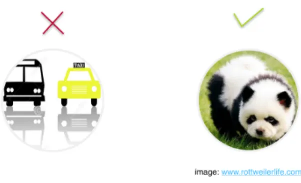
In the territory of computer vision, visual object classification is a theory about teaching computer how to classify objects from image or video visually, while fine-grained object classification aims at harder classification among categories which are both visually and semantically very similar. For instance, recognizing a car from buses (left part of Figure 1.1) is definitely common classification, while choosing a panda-faced dog from pandas (right part of Figure 1.1) can be regarded as fine-grained classification. The landscape of visual object recognition has recently been altered and pushed forward through the adop-tion of the deep convoluadop-tional neural network (DCNN) learning [2]. The recent results indicate that the performance of DCNNs can be pushed further by adding more training data, network layers and neurons [3, 4]. An increasing amount of data benefits DCNNs to learn even the finest class specific details to distinguish between visually similar classes and to become robust against imaging distortions, occlusion, pose changes and rigid and deformable deformations. However, with a limited amount of data or lack of resources for data annotation, “vision engineering” in the form of special architectures can be ben-eficial for mitigating the suffering from intra-class dissimilarity and inter-class similarity. This has been observed in fine-grained visual class detection that has recently become a hot topic [5, 6, 7, 8].

Figure 1.1.An example telling whether a classification case belongs to fine-grained classification.

In this thesis, we investigate several recent techniques in machine learning to improve the state-of-the-art DCNN methodology. It has turned out that the deep features, activations of the late hidden layers of a DCNN trained with ImageNet data [3], provide good generic features for vision tasks [9]. Task-specific optimization can be achieved by fine-tuning

(12)

T R A IN IN G T R A IN IN G T E S T IN G T E S T IN G

Image and label(s)

Image and label(s) Class detectionClass detection Rich spatialRich spatial

structure structure Specialization Specialization (<class>::<instance>) C la ss le ve l s e pe ra tio n C la ss le ve l s e pe ra tio n Instance detector Instance detector ::Downy-Woodpecker ::Bohemian-Waxwing do g :: sh ib a in u do g :: sh ib a in u bi rd :: bi rd :: B oh em ia n -B oh em ia n -W ax w in g W ax w in g bi rd :: bi rd :: D o w ny -D o w ny -W o od pe ck er W o od pe ck er Class Detection ::bird Class Structure detection DPM Object BBox Class Detection ::bird YOLO Object BBox Part BBox Specific Part BBox

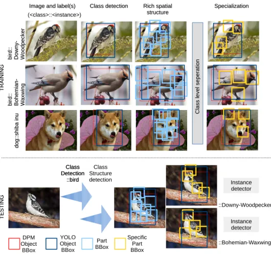
Figure 1.2.We extend the popular DCNN methodology by defining “latent sub-tasks” which

im-prove the deep fined-grained classification performance. Privileged information available during training (e.g., class hierarchy and annotated bounding boxes or object parts) is used to define the la-tent sub-tasks. During testing the privileged information is inferred automatically and contributes to the main task via structured decision making.

the ImageNet data based network with task-specific data [10]. In this work, we adopt this popular methodology to learn good deep features that already provide substantial boost over the fine-grained methods using conventional shallow features [5, 11].

To go beyond the state-of-the-art DCNN, we discover and exploit “ privileged informa-tion” that is auxiliary data available only during training. Such information is, for exam-ple, spatial location and structure of the class examples in the training set - spatial latent structure - and the class hierarchy of each fine-grained sub-class (e.g., bird::swan) - se-mantic latent structure. It is intuitively evident that knowing these during testing would improve fine-grained classification and this work shows that even estimating these “latent sub-tasks” provides a substantial performance improvement. Similar results have been reported in biometrics where face recognition benefits from accurate detection of facial landmarks [12] and facial age estimation benefits from detection of semantic information

(13)

such as the gender or the age group [13, 14]. The reason for the improved performance is in the fact that discriminative information extracted from “latent sub-problems” can pro-vide strong “soft prior” for final decision making. In this work, we assume that accurate and discriminative parts play a vital role in fine-grained visual categorization. Neverthe-less, annotating parts by humans is time-consuming and less reliable. On one hand, the definition of object parts contributing to fine-grained classification can vary from persons to persons, which can require a strong prior background in the field. For example, for classifying fine-grained bird breeds, even non-experts hardly distinguish one class from another. With the helps of experts, annotating a number of object parts for each image is laborious and poorly scaled to large-scale problems.

In this thesis, we propose a novel framework for fine-grained categorization by automati-cally discovering and utilising discriminative parts of the fine-grained object. To this end, we attempt to use the under-parts of Deformable Part Models (DPM) [15] as annotation-free object parts and then we consider part specialisation by discriminatively selecting and combining object-specific parts to boost categorization performance. The pipeline of our method is illustrated in Figure 1.2. In our experiments, the proposed framework based on privileged learning consistently improves the fine-grained image classification on the popular fine-grained datasets indicating that exploiting latent sub-tasks is beneficial for deep visual classification: Oxford-IIIT Pet [5], Columbia Dogs [11] and Caltech-UCSD Birds-200-2011 [16].

(14)

1.2

Contributions and Thesis Outline

The novelties and contributions are:

• We extend the popular deformable part model to learn rich and specialised spatial structures of fine-grained classes - a spatial structure sub-task.

• We propose a semantic sub-task by exploiting available class hierarchy.

• We propose a structured decision making approach that incorporates the two latent sub-tasks into the learning of the main task – fine-grained classification.

• We demonstrate clear performance boost using deep structured privileged learning (DSPL) on three popular fine-grained benchmarks.

The remaining parts of the thesis are organised as the following. Chapter 2 describes related works and reviews on object classification, several popular datasets involved, basic concept of a number of general neural networks works. Chapter 3 investigates the design of our structured privileged learning framework part by part. In Chapter 4 we conduct the experiments, including state-of-the-art results, analysis and comparisons among different methods. In Chapter 4.8, we give a more general form of structural decision-making and privileged learning, which can be applied in other applications. In Chapter 5, the conclusion will be summed up, and also the shortcoming, the advantages and the potential future directions will be discussed.

The next part will give the necessary mathematical background of deep neural networks and their popular variations, explaining how they learn and infer, as well as some motiva-tions why these methods are suitable for classification problem .

(15)

2

RELATED WORK

This chapter investigates related works which are focusing on object classification and fine-grained classification. Then, we introduce the benchmarking datasets used in this work – Caltech-UCSD Birds-200-2011 (CUB-200-2011) [16], Oxford-IIIT Pet [5] and Columbia Dogs [11]. Furthermore, the basics of neural networks are presented, which cover two types of neural networks (AlexNet [3]and VGG [1]) used in this framework. Although recursive neural network (RNN) is not directly applied, we borrow some idea from the design of it and may include RNN in our framework in our future research. In the final part, toolboxes and the corresponding configuration of our approach will also be explained.

2.1

Deep Learning

Before going into deep learning, we introduce neural network first. In terms of machine learning and cognitive science, neural network is a family of statistical learning model inspired by the biological neural network. Since neural network was proposed several decades ago [17], it has been seen that neural network suffered from local extreme opti-mization, insufficient training set and vanished back propagation. Deep learning (neural network with more convolutional layers and fully-connected layers) resurged in recent years: Hinton et al. [18] proposed a brand-new way to initialize weights of CNN us-ing restricted Boltzmann machine, which experimentally leads to a better optimisation performance, which was also achieved later by Vincent et al. [19] using autoencoder. Then, a well-known work published by Krizhevsky et al. [3], showing that large-scale supervised deep neural networks empirically outperform those traditional methods using feature engineering.

Classification and Fine-grained Classification – Prior to the deep learning paradigm [2, 3, 20] there were several popular approaches to visual object categorization, in particular, visual Bag-of-Words (BoW) [21, 22] and the deformable part model (DPM) [15]. BoW and DPM utilized traditional features, e.g., SIFT [23, 24, 25] or HOG [26], and support vector machine (SVM) learning. Advanced versions of these have been proposed for fine-grained classification [11]. These works, as well as Gavveset al.[27] and Zhanget al. [6] provided good results, but require more supervision to select semantically mean-ingful parts. Yang et al. [28] learned the parts in the unsupervised manner, but their model is inferior to the deformable-part model used in our work and therefore their

(16)

re-sults are not competitive. The landscape of visual classification was altered in 2012 by the seminal work of Krizhevskyet al.[3] which introduced a deep convolutional neural network (DCNN) architecture. Their approach was soon adopted for fine-grained classi-fication [6, 7, 8]. The state-of-the-art methods first extract activations of the late hidden layers of a DCNN trained with ImageNet data [3] - generic deep features [9] - which can be further improved by fine-tuning the network with task-specific data [10]. For classifi-cation, the last layer of the trained DCNN or one-vs-all support vector machines (SVMs) are used. Further improvements can be achieved by adding special processing stages prior or after the DCNN feature extraction [6, 7, 8]. It is important to notice that the fast progress of DCNN architectures provides improvements that seem to go beyond adding novel processing stages. For example, the performance improvement by dedicated part selection in [29] was achieved also by switching to a more recent DCNN [1]. Similarly, our proposed processing stages also improved the results , which are in Chapter 4.

Beside recent developments, there are also other main concerns that need to be outlined. The first is that deep features learned by deep learning can skip the period of preparing hand-crafted feature, which is a quite heavy work and can takes much time. One ob-vious drawback of hand-crafted feature is that hand-crafted feature needs to be tailored for different modality (images, voice). The other reason can be that compared to shallow hand-crafting feature, deep feature can capture coarse-to-fine information, in other words, information on multiple levels, from simple edges and colour feature to abstract object-based feature. This thesis will show how supervised and unsupervised learning can be easily applied in a variety of classification tasks. In particular, like human can process an image as discrete local RGB points, or as overlapped objects, CNN can make decision based on meaningful representations from multiple levels.

2.2

Structured Learning

Our work was inspired by the recent results in face biometrics where certain tasks, such as identification and age estimation, can be seen as fine-grained tasks. It has been found that face alignment based on spatial structures (facial landmarks) [12] and semantic pre-classification, e.g., to the gender or age groups, improves the final classification [13, 14]. More recently, structured ontological semantic structures have been used in the fine-grained classification of street view images [30]. According to the recent machine learn-ing literature, semantic and spatial annotations can be stated as “privileged information” which is available only during training [31, 32, 33]. We exploit the spatially-localized and discriminatively-selected object parts (shown in the2nd column in Figure 3.1), and

(17)

formulate the fine-grained classification problem as structured decision-making that is successfully used in influence diagrams and decision networks [34, 35].

2.3

Datasets

2.3.1 Datasets for Fine-Grained Classification

As we mentioned, fine-grained object categorization is a classification task aiming to dis-tinguish the breed or species of objects from an image, thus specific datasets are necessary for deep-learning-based approaches. There are many datasets used for fine-grained visual categorization including the Oxford-IIIT-Pet dataset [5], the Columbia Dog dataset [11], and the Caltech-UCSD Birds-200-2011 [16]. The split of the trainset and testset of these three datasets were kept same as the original works [5, 11, 16] do.

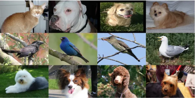
Oxford-IIIT Pet dataset [5]: contains 37 fine-grained pet categories with roughly 200 images for each class. Among 37 classes of pets, 12 categories belong to the cat parent category, and the remaining are dog breeds. The Columbia Dog Dataset can be found in Figure 2.1.

Columbia Dog Dataset [11]:contains 8351 crowdsourced images of 133 American Ken-nel Club (AKC) recognised dog breeds downloaded from Google, ImageNet [36] and Flickr. The examples of Oxford-IIIT Pet Dataset and the Columbia Dog Dataset can be found in Figure 2.1.

Caltech-UCSD Birds-200-2011 Dataset1: is another fine-grained dataset in distinguish-ing species of birds. It contains11,788images from200species in total. For each image annotated part locations and one bounding box are provided. The challenges lies on that certain bird species vary dramatically in appearance in leather colours (e.g.sparrows), and bird can act in different varying pose as soft cat body does. Even for bird experts, some pairs of bird species are nearly visually indistinguishable, such as the sparrow species. Intra-class variation is high due to the reasons mentioned, while inter-class variation is low as some species look quite similar. The examples of Caltech-UCSD Birds-200-2011 Dataset can also be found in Figure 2.1.

(18)

Figure 2.1. The selected Examples of the OXIIIT Pet Dataset (the top row), the Caltech-UCSD Birds-200-2011 Dataset (the middle row), and the Columbia Dog Dataset (the bottom row).

(19)

2.3.2 ImageNet Dataset

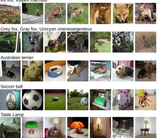
As our models use the pre-trained weights learned from ImageNet, here we introduce this well-known deep learning benchmark – ImageNet Dataset. ImageNet dataset [36] is a large-scale benchmark collected and released for ImageNet Large Scale Visual Recogni-tion Challenge, with several millions of images of 1000 kinds of objects,e.g. vehicles, animals, and daily goods. This is the main benchmark of image classification and object detection, on which researchers use to develop new algorithms. This dataset contain1.2

million samples for training, 50000 for validation, and 100000 for testing. Figure 2.2 shows samples from ImageNet. We observe that the ImageNet Dataset holds massive images for each class, while the inter-class variance is noticeable.

Kit fox, Vulpes macrotis

Grey fox, Gray fox, Urocyon cinereoargenteus

Australian terrier

Soccer ball

Table Lamp

(20)

2.4

Neural Networks

In this section, the basic introduction to the most important neural networks structures will be given: Multi-Layer Perceptron, Convolutional Neural Network, Recurrent Neural Network, and also Long Short-term Memory Machine.

2.4.1 Single Neuron

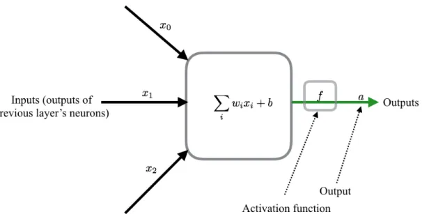
All mentioned networks are based on single neurons. Figure 2.3 gives an illustration of how a single neuron works, i.e. the input is transformed into output via an activation function. Defining the inputs n-dimensional vector, the calculation follows the equation below:

a=f(wTx+b), (2.1)

wherefmeans a non-linear activation function. From the biological prospective, the acti-vation functionf is designed to digitally imitate human neuro’s producing spike in some certain frequency. Normally, a typical choice of activation function is sigmoid function f (Equation 2.2) [37], as this function can absorb a real-valued number and produce a normalized value between0and1, which is showed in the left part of Figure 2.4. There are also other activation candidates,e.g. tanhfunction (Equation 2.3),hard tanhfunction, and also rectified linear function: f =max(x,0).).

σ(x) = 1/(1 +e−x) (2.2)

Some of them like tanh are nowadays applied a lot as it shows better empirical perfor-mance and faster to refer.

tanh(x) = (1−e−2x/1 +e−2x) (2.3) The output of a single neuron is given to another single neuron or multiple neurons as input, forming a net-like topology, which is the basis of a Multi-Layer Perceptron (MLP).

(21)

Figure 2.3. The mathematical model of a single neurone with inputs, activation function and output.

(22)

2.4.2 Multi-Layer Perceptron (MLP)

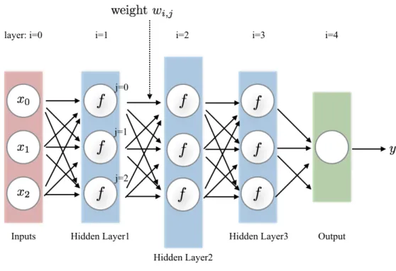
A Multi-Layer Perceptron can learn a complex and non-linear mapping functionf a sin-gle neuron cannot do [17] as MLP contains more complex architecture: an acyclic graph consisted of layers of single neurons. The organisation of MLP is showed in Figure 2.5.

Activation Function All hidden layers and the output layer can be equipped with an activation function like sigmoid σ. The necessity of activation function lies on that the activation function effectively controls the range of value, which makes technical imple-mentation easier.

Figure 2.5.A MLP with 3 inputs, 3 hidden layers of 3 neurons each layer, and 1 output.

Forward Pass The forward pass of a fully-connected layer corresponds to one matrix multiplication followed by a bias value and an activation function. The whole forward pass of MLP is repeated matrix multiplication interwoven with activation function. Here, we define the M-dimensional input vector asx = {x1, x2, , , xM}, the learnable parame-ters of network as Q-by-M weights matrixw = {w1,1, w2,1, , , wQ,M}and Q-dimensional bias vectorb = {b1, b2, , , bQ}, so the forward pass of the first hidden layer can be com-puted by:

(23)

a=f( Q X j ( M X i wj,ixi+bj)), (2.4)

where the activation functionf is non-linearity that is applied elementwise andarefers to the activation value. Likewise, the forward pass of the second hidden layer follows same equation as Equation 2.4, until the final output is given by:

y= K X j ( P X i wj,iai+bj), (2.5)

where the termK andPrefer to the dimensions of output and feature of last hidden layer respectively.

Representation Power – Trained using Back Propagation (BP) algorithm (explained in Section 2.5.1), the MLP shows decent performance on a wide selection of recognition tasks [38] for its representation power on a family of functions. How big is this family? This is investiaged in [39], which also arise another problem – what are functions that cannot be modelled by MLP. Mathematically and theoretically, a two-layer MLP can model any continuous functions. The reason people prefer deeper (more layers) one is that from an empirical observation deeper one performs better than shallow one. In another way, a shallow three-layer MLP is suitable for some tasks, but adding layers does not necessarily boost performance. Simply adding more layers may even lead to over-fitting, which can be interpreted as a network with high representative power fitting well the noise data contains, rather than data itself.

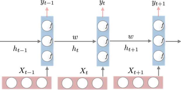
2.4.3 Recurrent Neural Network (RNN)

Recurrent Neural Network (RNN) is a specific neural network where connections between units form a directed cycle. We do not apply RNN in this work, but we discover its usefulness when we want to extend our work to sequence processing (e.g. video). Thus, we investigate RNN and LSTM here. RNN is capable of conditioning the model on all previous temporal information. The basic architecture is unfolded and illustrated as Figure 2.6 from which we can see same neurone unit is repeated in time steps. Each neurone consists of matrix operation with weights w followed by a non-linearity (for instance sigmoid). The input vector xt in time stept, will be used to feed the neurone,

(24)

together with the outputht−1from the neurone in time stept−1. Physically, the neurone

does not change, but its weightswchange recursively.

Figure 2.6.RNN architecture unfolded in three time steps.

The inference process of RNN can be summarized using the equation below:

ht=σ(whht−1+wxxt), (2.6)

yt=sof tmax(wsht), (2.7)

where wh, wx and ws represent weights matrices for conditioning the previous output, conditioning the input vector and mapping to output space respectively,ytrefers to clas-sification value at time-stept, andxtis input.

Gradient Explosion & Vanishing

RNN can be very long (for instance over 1000layers), as it is single unit as a loop over time steps and it is designed to carry or propagate information through massive steps theoretically. But in practise, there exists one problem preventing RNN from being too long: in back-propagation, gradient vanishes or explodes through a very long time series. Here are some formulations where we can gain intuition about this problem. Let’s define Etas the RNN error in time stept. Till the time stept, the gradient of the RNN error on

(25)

wxcan be expressed as: dE dwx = T X t=1 dEt dwx = T X t=1 t X k=1 dEt dyt dyt dht dht dhk dhk dwx = T X t=1 t X k=1 dEt dyt dyt dht ( t Y j=k+1 dhj dhj−1 )dhk dwx . (2.8)

Here we will not give strict mathematical induction, but from the equation we can find if _d_hjdhj

−1 does not wander around numeral 1 (which is determined by wx) and (t−k) is

exactly big enough, then dE

dwx is squeezed into nearly zero or zoomed out to be infinite value.

(26)

2.4.4 Long Short-Term Memory Machine (LSTM)

The motivation to introduce LSTM [40] is that LSTM is an extension of RNN importing more constraints to handle the gradient explosion & vanishing problem. LSTM can also be regarded as a neural network with three specific gates (Input Gate, Forget Gate, Output Gate) added on the basis of RNN. Before simply listing all mathematical formulation, it is better to look at the structure of an LSTM from where we may gain some intuition.

Figure 2.7.A LSTM network consisted of five computational units. Thetanhrefers to point-wise

tanh operation, and◦denotes the Hadamard product.

The novelty in structure of LSTM can be analyzed in following steps:

1. Memory Generation Unit: Similar to the basic unit of RNN, this unit use the data at time stept xtand past hidden state ht−1 as input. What is different is that

this unit generates some kind of new memoryc˜t, rather than a new hidden stateht. Technically, we can sayc˜tcontains some information from of the new dataxt.

2. Input Gate: The function of this gate answers a question (whether xt matters or not) considering the input data xt and the past hidden stateht−1. If the answer is

not at all, the indicatoritgiven by this gate is set to0, thus no information fromxt can be reserved.

(27)

3. Forget Gate: Forget Gate works like Input Gate but in a different way. Input Gate controls the information of the input dataxtleaked in, while Forget Gate determines the amount of the past memoryct−1 which will be forgotten. If Forget Gate is on,

the wholect−1will be demolished.

4. Memory Fusion Unit: Memory Fusion Unit fuses two sources of memory (the past memoryct−1and the new memoryc˜t) into the current memoryct.

5. Exposure Gate:Exposure Gate or Output Gate outputs indicatorotto separate the final hidden statehtfrom the current memoryct, as there is no need to preserve all information ofct.

The reason behind inserting memory-related operations is that important gradient can be stored in memory cells without dissipating quickly.

2.5

Convolutional Neural Network (CNN)

As convolutional Neural Network (CNN) is a necessary part of our method, we give a comprehensive investigation on it in this section. Convolutional Neural Network (CNN,) is quite similar to MLP in Section 2.4.2 : it consists of neurons that have weights and bias, including some loss function and fully-connected layers. Like MLP, CNN also obeys the rule that a raw pixels from one side are mapped to activation values on the another side. The difference of CNN with MLP lies on two points: 1), CNN uses convolutions instead of fully-connected layers. 2), CNN uses pooling to compress representations. Below, two layers for convolution and pooling will be proposed, and a visualization of CNN repre-sentation will be given. This is a practical structure we use quite often in the whole of this thesis. Firstly we introduce some basic aspects of CNN.

Convolutional Layercontains convolution operation which does the most computational heavy work. This operation is represented in Equation 2.9. Put it in a simple way, the analogy behind is using learnable feature filters to spatially multiplicate regions of input which may be raw images. Considering the region can be everywhere, we need to slide the filter along the width and length of the image to get activation map, shown in Figure 2.8.

(28)

Figure 2.8. A sample of convolutional layer architecture. Parameters are choose from VGG-19layer [1]. After convolution by filter of shape (64,3,3,3) (refers to64filters with width3, height

3and3channels), a raw image of shape (3,224,224) (refers to an image with width224, height

224and3channels) is mapped into a feature of shape (64,224,224).

an_j =max(0, K

X

i=1

an_i−1wn_ij), (2.9)

where the superscriptnis the next layer ofn−1,xn−1 _{refers to feature map or raw image}

from layer n−1, and wn

j representsjth filter of nth layer. A strength of convolutional layer as compared to a fully-connected layer is that each neuron is only connected to a local region of input, that is called the receptive field. Another advantage is parameter sharing, which is constrain each neurone in the convolutional layer to use the same set of weights and bias.

Pooling LayerThe function of the pooling layer is aggregating spatial feature, lowering the size of representation , and make smaller the parameter size of the whole neural net-work [3]. This layer achieves the effect of pooling by doing Max or Mean spatially, which make the network more general and robust.

Feature Visualization

Visualization is a notable approach to understand convolutional neural networks, and sev-eral methods have been developed in [41].

(29)

Figure 2.9.An example of pooling layer. Parameters are chosen from VGG-19layer [1]. Averag-ing or choosAverag-ing maximum value of4nearby pixels, the raw image of shape (3,224,224) is pooled into the feature of shape (3,112,112).

first CONV layer, as this layer is relatively low and close to raw pixel, and its represen-tation is quite interpretable. As shown in Figure 2.10, smooth colour or edge filters are exhibited without interference of noise, which can to some extend prove that the model is trained in a correct direction and for long enough.

Visualization of Activation – Checking the layer activation matrix is another common strategy to get insight of the question: what the data flow looks like in forward pass. Here it needs to be mentioned that this approach is of intuitive grasp, but on the other side, adaptive to input. In Figure 2.11, it gives the illustration of a shallow activation matrix and a deeper one.

Here we visualize some parts of the well-known CNN models -AlexNet [3] and VGG [1]. For more details about these models, we refer reads to the original papers [3, 1].

(30)

Figure 2.10. visualisation of 1st CONV filter of AlexNet. Notice that pattern inside this image is smooth and pure, indicating at least the weights of first convolutional layer converged well.

Figure 2.11. An example visualisation of 1st CONV activation and 4st CONV activation matrix

of AlexNet with input is one image of a cat. Although many boxes are black (activation value equals zero), we can still find that some boxes contain the general shape of a cat.

(31)

2.5.1 CNN Back-Propagation

In CNN, backpropagation is a method to compute the gradient of target error on different network parameters, which is executed in the inverse direction of feedforward process [17]. Feed-forward and back-propagation can be considered as two sides of a problem (inference and learning). Technically, the whole process of back-propagation is a way of calculating the gradient of the final error (classification error or regression error) on weights in different layers via recursive application of chain rule. The gradient on each variable can reflect the degree to which the variable can affect the final expression. Con-sider a simple compound function of only one number,f(x) = a(b(x)). The chain rule can be expressed as: df

dx = da db

db dx.

Now we apply this into practice. Let’s assume an example shallow three-layer MLP. The feed-forward process is implemented as matrix operations as follows:

h1 =w1×x+b1, a1 =σ(h1), h2 =w2×a1+b2, a2 =σ(h2), score=w3×a2 +b3, (2.10)

where wi and bi terms denote connection weights and bias of multiple neurons in the layeriwhich is multiplied with and summed respectively, and the notationσrefers to the element-wise sigmoid function (Equation 2.2).

Assume a loss function outputslossbased on the inputscore. We compute gradient using the chain rule in the inverse order of the Equation 2.10:

(32)

d loss d w3 = d loss d score ×a2.T, d loss d b3 = d loss d score, d loss d a2 =w3.T × d loss d score, d loss d h2 = (1−a2)•a2• d loss d a2 , d loss d w2 = d loss d h2 ×a1.T, d loss d b2 = d loss d h2 , d loss d a1 = (w2.T ∗ d loss d h2 ), d loss d h1 = (1−a1)•a1• d loss d a1 , d loss d w1 = d loss d h1 ∗x.T, d loss d b1 = d loss d h1 , (2.11)

where the full equation seems similar. Here we focus on the backward flow, without explaining which loss function thelossis from. In most cases, thelossis given by cross-entropy loss or mean square error loss combined with regularisation loss. The partial derivative oflosswith respect to the weightwi of the layeriand the learning rate set in CNN controls how large thewiis updated.

(33)

2.6

CNN Optimisation

In our context, optimisation is a general term referring to the adaptation of a particular set of parameters to make score better agree with ground truth labels in training data, thus minimizing the loss function. Given a convex function (e.g. SVM cost function) as loss function, there are many methods minimizing this type of functions. However, in neural networks, our loss function will be non-convex in high-dimensional hyperspace. Below, we will give several strategies to optimise the non-convex loss function.

1. Random Local Search: This strategy starts with a randomly initialized weightsw, then replaces it with (w+δw) where δw is small randomly initialized matrix, if

(w+δw) leads to lower loss score. This is a straight-forward choice (better than random search), but quite computational wasteful.

2. Partial Derivatives:This strategy updates weightswin the direction of the steepest descend, which is reflected by the partial derivativesdwof the loss function. This always follows the steepest direction which seems optimal, but cannot guarantee that it can reach the global optimal point.

3. Stochastic Gradient Descent (SGD): SGD also uses partial derivatives in batch-wise way. In large scale recognition tasks, it seems to waste a lot of time validating complex loss function over millions of samples one by one. Stochastic gradient de-scent (SGD) is introduced to address this problem. In the presence of SGD, the loss will be computed batch-wisely, making the best use of vectorized programming, and resulting in shorter running times and shorter converging time.

(34)

2.7

SVM Classifier

When facing a classification problem, which is the main target of this thesis, what we care about is the accuracy. There are some "good enough" classifiers already,e.g., Naive Bayes [42] for data with high bias and low variance, Logistic Regression [43] which can easily get updated when new data comes, Decision Trees which is not parametric and can easily handle feature interactions, and also support vector machine (SVM) [44] which is designed and upgraded to deal with non-linearly dividable data. It often says, better data beats better classifiers. In other words, when a dataset is huge enough, the performance does not vary dramatically whichever classifier we use. In this thesis, we adopt SVMs to do classification on deep representations produced by DCNNs.

2.7.1 Support Vector Machine (SVM)

Traditional SVM is what we called the binary SVM. Given a data set,Ω = {(x1, y1),

(x2, y2), , ,(xn, yn)}wherexn∈Rdrefers to a set of coordinates in input space andyn ∈

{−1,1}is the class label of pointn, the advantage of SVM is that it can create a linear or non-linear decision boundary that separates two types of points. The closest distance from two class of points to the decision boundary is equal, thus the final constructed decision boundary keeps the maximal margin between two classes. The object function of SVM is shown below: min w,b,ξ 1 2kwk 2₊_CX i ξi, s.t. yi(w·Φ(xi)−b)≥1−ξi, ξi ≥0 . (2.12)

where w, b and Φ are SVM weights, bias and a kernel function. ξi is introduced for preventing the over-fitting problem in case decision boundary is adapted to outliers, and the constantCdetermines the trade-off between maximising the margin and misclassified outliers. The optimisation can be solved by using Lagrange multipliers, and the decision of one pointxis given by:

f(x) =sign(

n

X

i=1

aiyiK(x, xi) +b), (2.13)

where eachai is Lagrange multiplier,K(x, xi)equals toΦ(x)TΦ(x)which is also known as kernel function.

(35)

2.7.2 One-class SVM

Here we introduce one-class SVM. Compared to binary SVM, one-class SVM can handle one situation very well: you only have data of one class and the goal is to test new data and found out whether it is alike or not like the training data? There are two mainstreams of one-class SVM: Support Vector Data Description by Tax and Duin [45] (SVDD) and Support Vector Method For Novelty Detection by Schölkopf et al. [46]. SVDD aims to find minimized hypersphere which contains all data points except those outliers. A hypersphere can be parameterized by a sphere center a and a radiusR > 0. Similar to traditional SVM, this sort of SVM also requires that the distance from the data pointxito some certain destination is not bigger than set distance (for instanceR, meanwhile slack variable ξi combined with penalty value C are imported for providing soft margins for outliers), thus the solution procedure is formulated as:

min R,a R 2₊_C n X i ξi. s.t. kxi−ak 2 ≤R2+ξi, ξi ≥0 . (2.14)

Upon getting hypersphere center positiona, the conclusion can be induced from whether the pointxlies inside the hypersphere. Different with SVDD mentioned above, Schölkopf et al.[46] introduced a new specific one-class SVM, which builds a hyperplane maximis-ing the distance of it to the origin. The correspondmaximis-ing minimization problem is also quite similar to original SVM equation:

min w,ρ,ξ 1 2kwk 2 + 1 νn n X i ξi−ρ, s.t.(w·Φ(xi))≥ρ−ξi, ξi ≥0 . (2.15)

where the parameterνcontrols the trade-off between the fraction of outliers and the num-ber of training vectors. A hyperplane parameterized bywandρis constructed to separate all points from the origin point. Here please note that we mention two one-class SVM ap-proaches just for completeness. In practice, we apply the one-class SVM implementation provided by liblinear-1.5-dense-float (https://github.com/BVLC/DPD/tree/ master/thirdparty/kdes_2.0/liblinear-1.5-dense-float), which sup-ports SVDD. While kernel function is a key component of SVM for great power dealing with high-dimensional data. We skip introducing kernel function as it is not our focus.

(36)

2.8

Detection Framework

From the prospective of computer vision, detection refers to the vision task of localising where is the object if given a raw image. The output of detection is a outline box bounding the object. In this section, we will give a brief introduction to common detection methods.

Detection can be made much easier if the examples can be aligned, located or rigid parts detected. In [5], animal (e.g. dog and cat) faces were detected by a sliding window de-tector of HOG features [26] and then a deformable outline was extracted by using the detected face as a segmentation seed. The downside of their approach is that the face must be clearly visible and outline annotations are needed for training images. More-over, discovering class-discriminative object parts automatically (i.e. without any part annotations during training and testing) is even more challenging to boost categorization performance.

2.8.1 Deformable Part Model (DPM)

The deformable part model (DPM) by Felzenszwalb et al. [15] is a part-based extension of HOG which can unsupervised learn discriminative deformable parts and even multiple “modes” of object appearance (e.g. frontal view bike and side view bike). DPM requires class images with annotated bounding boxes for training. Semantically meaningful parts can be used, but that requires their manual annotation [6].

The most important parameter is the number of modes that is fixed by default, but should actually reflect the complexity of each class. Each class-specific DPM model is defined by a root filter F0 and a set of part models (P1, . . . , Pn) where the number of the parts is fixed to n = 6by default. Multiple class “modes”, e.g., different 3D viewpoints, can be implemented by using multiple DPMs for each category. The parts are defined by the parametersPi = (Fi,vi, si, ai, bi). Fi is a filter for thei-th part, vi is a two-dimensional vector specifying the (optimal) location of the part with respect to the root part, si is the size of the part box and ai and bi are two-dimensional vectors describing the quadratic score for the displacement of the i-th part. All these parameters are learned from the training set using the latent-SVMs [15]. The output of the DPM search for a test imageI are the locations and scales of the root (red bounding box in Figure 2.12) and each part

(37)

Figure 2.12.Examples of the DPM learned human models using8latent parts.

Figure 2.13. Examples of the YOLO learned human models using an end-to-end CNN structure.

Image is from [47].

2.8.2 YOLO detector

The YOLO detection framework is an extremely efficient generic detection framework [47], which skips time-consuming scanning region proposals, and uses a GoogLeNet-similar CNN to produce bounding boxes and class probabilities in an end-to-end way (illustrated in Figure 2.13). The comparative evaluation in [47] shows that the YOLO detector is superior to DPM. YOLO gives object bounding box similar to that of DPM, but without bounding boxes for latent parts. Here we do not focus on the principles of YOLO. For more details, we refer our readers to [47], which analysis this structure part by part and makes a comprehensive comparison with other state-of-the-art detection framework.

(38)

3

METHODOLOGY

CNN Layer:fc7 … Specialization Root Parts

Figure 3.1.Rich part-based spatial structure is learned from training data using only bounding box

annotations. Multiple models in DPM, “modes”, provide robustness to deformation and viewpoint changes, and latent class-specific part specialisation provides discriminative information for fine-grained classification. For mitigating the suffering of false detection by DPM, YOLO detector is employed for foreground refinement to further boost categorization performance. Class-sensitive parts can be selected by either discriminative combination using one-class SVM (top) or exhaus-tively searching (bottom).

Figure 3.1 illustrates the workflow of our rich spatial structure learning, which can be divided into the following phases:

1. latent object part discovery presented in Section 3.1;

2. class-specific part selection (part specialisation) in Section 3.2;

3. fine-tuned DCNN features to encode spatial structure information in Section 3.3.

(39)

Figure 3.2.Examples of the DPM learned class-specific part models.

3.1

Latent Part Discovery

In fine-grained classification, an image hard to classify may include noisy background, ambiguous repetitive patterns and pose variations. These challenges make fine-grained classification even harder. As subtle differences exist in highly localised regions, we locate the object and its latent parts (informational patches) using two popular detection frameworks. To keep the level of supervision reasonable, we adopt the DPM and optimise its parameters for each class of dataset. In our experiments, each class-specific DPM model is defined by a root filterF0and a set of part models(P1, . . . , Pn)where the number of the parts is fixed ton= 6by default. For each image, a DPM model gives7bounding boxes as output (1object box and6part boxes). In Figure 3.2, we visualize some examples of latent parts discovered by DPM (some of them only contain less than7parts selected usingpart specialisationin Section 3.2).

It is evident that accurate object location is vital in recognizing object class [48], but the conventional DPM is less favourable for very deformable animals (e.g. birds). To

(40)

achieve more accurate detection results, we adopt YOLO [47] in addition to the DPM. The comparative evaluation in [47] shows that the YOLO detector is superior to DPM. In view of this, we employ both models as DPM can intrinsically model latent parts without using ground-truth part annotations and YOLO detector can provide precisely-positioned object bounding boxes. Specifically, we extract feature from both output (bounding boxes) of DPM and YOLO to represent the global object and incorporate latent deformable parts of DPM into the framework for providing localised discriminative information from parts.

3.2

Part specialisation

The output of Section 3.1 are class object and class specific spatial parts (nc bounding boxes in total for class c) defined by the root and part locations and their spatial extend (sizesi):

{I1, I2, . . . Inc}={(v1, s1), . . . ,(vnc, snc)} . (3.1) These can be converted to the part windowsI0, . . . , Inc from which the deep featuresx are extracted (see Section 3.3 for more details):

x= (x1, . . . ,xnc) =

{DCN Nf c6(I1), . . . , DCN Nf c6(Inc)}

. (3.2)

The concatenated feature vectorxencodes the deep features extracted from part locations and can be directly used to train a classifier. However, during the experiments we found that the performance of the latent sub-tasks, i.e. part detection and selection, can be im-proved by simple re-weighing which consequently improves the performance of the main task of fine-grained classification - one decision stage in structured learning influences the overall performance. We refer to our weighting method as “part specialisation”. The method is motivated by the fact that for different sub-class the importance of each part varies. The part feature re-weighting is related to the feature selection [47, 49, 50, 51]. We adopt the following procedure for feature re-weighting [52]:

ˆ

X = cT ·I ·XTT = [c1·x1 . . . cnc·xnc] (3.3) where X is a(D×nc)feature matrix where the D-dimensional feature vectorsxi are concatenated column-wise, c ∈ _Rnc _{is the weight vector of the same dimension as the} number of parts andIis(nc)×(nc)identity matrix. The extreme values of the weights are ci = 1for the maximum importance andci = 0for a part that can be omitted for that class

(41)

(see Figure 1.2 for example). The straightforward solution is to determine class-specific optimisation ofcby cross-validation. More advanced procedure of “part specialisation” attempts to introduce one set of scalar-valued part weights instead of binary weights to maximize the gap between the decision values for true class and false class, which can thus be formulated into one-class SVM problem. In other words, as one-class SVM can discriminatively determine the probabilities of testing samples belonging to the positive class to fit positive training samples, we can thus employ it to select discriminative parts by minimising the object function below:

c∗ = [c∗₁, c∗₂, , c∗_nc] =argmin( N X i X j6=J max(1− nc X k ckeij,J(k)) 2 +Ckck1), (3.4)

where i, j, k and J are the index of the training image, the image class, the index of selected part and the ground truth class of theith image respectively.Cdenotes the trade-off parameter and ei_j,J refers to the loss between misclassified classj and ground truth classJ as follows:

ei_j,J(k) = (w_i,k,JT −wT_i,k,j)fi,k (3.5) Thefi,k represents D-dimensional deep feature extracted from the partk of the imagei, of which the extraction procedure will be investigated in the next section (Section 3.3).

3.3

Deep Feature Extraction

Following the success of very deep neural networks for object detection tasks [1, 53], we used the 19-layer DCNN model (configuration "E" in [1]) trained on ILSVRC-2014 ImageNet data. The DCNN learns generic and discriminative features for visual recogni-tion, but we also experiment DCNN fine-tuning to generate more dataset-specific features in our experiments. To achieve this, we follow the transfer learning procedure: alter-ing final inner-product layer with a much quicker learnalter-ing rate (e.g. 10 for the learning rate in Caffe), updating other weight-carrying layers (convolutional layer, inner product layer) with a moderate or slower rate (e.g. 1 for the learning rate), and then complet-ing fine-tuncomplet-ing procedure on our three datasets respectively. If part boundcomplet-ing boxes are achievable during the training phase (produced by DPM), separate fine-tuning will be per-formed only for parts. Instead of extracting DCNN feature from global region (i.e. the whole image), we use DCNN to extract features for root and part locations from the "fc6" 4096-dimensional layer.

(42)

Priviledged Info (super-class level)

Images

Priviledged Info (sub-class level)

Super Class Sub Class

Figure 3.3. We adopt the privileged learning principle and semantic pre-classification to learn

strong SVM classifiers for super class and sub class detection.

3.4

Privileged Learning

The important question is how we can utilize privileged information – information avail-able only during training (Figure 3.3). In this work, privileged information we want to apply can be the discovered and selected bounding boxes for spatial structures. Detection of privileged information from training images forms latent sub-tasks that contribute to the main task of fine-grained classification in the form of structured privileged learning and decision-making.

Since the introduction of the concept of learning using privileged information (LUPI) [31], there has been a growing body of methods to implement the learning paradigm [32, 33]. In the multi-class setting the golden standard classification approach is to trainN one-vs-all support vector machine (SVM) classifiers producing the output Y = {1,0}(yes/no) and learning is implemented by minimizing a convex cost function, e.g. the hinge loss function

`(y) = 1−y·f(x) . (3.6)

Privileged information in the above case means that during the training phase, optimisa-tion of (3.6), we have available auxiliary “privileged” informaoptimisa-tion in the form of vectors pi associate to all training samples xi. The easiest implementation of the learning us-ing privileged information is to concatenate these extra information vectors to the data features vectors [31], but that would be problematic in the testing phase where this infor-mation can be not available. Pechyony and Vapnik [32] proposed the SVM+ algorithm

(43)

where the convex SVM optimisation problem [54], min w,b,ξ 1 2kwk 2 +CX i ξi s.t.yi(w·Φ(xi)−b)≥1−ξi, ξi ≥0 . (3.7) is recast as min w,b,w˜,˜b,ξ˜ 1 2kwk 2₊ 1 2kw˜k 2 ₊_CX i ˜ ξi s.t. yi(w·Φ(xi)−b)≥1−ξ˜i, ˜ ξi ≥0 . (3.8)

where the slack variableξ˜isa correcting function

˜

ξi = ˜w·Φ( ˜xi) + ˜b . (3.9) The slack variable in (3.9) “corrects” the discriminating hyperplane in the space of the privileged features, that is, if we can achieve a small loss in the correcting space of privi-leged informationx˜i ∈ P, then we should also achieve a small loss in the original decision spaceX. It is important to notice that the classifier does not need the privileged informa-tion in the testing stage since it learns a direct mappingf(x)→yfrom the feature to the decision space.

3.5

Multi-Stage (Structured) Privileged Learning

We found the embedded form of the SVM+ in (3.8) and (3.9) inferior to the multi-stage form that we describe next. The multi-stage form forms the structured privileged learning and is more intuitive: train separate classifiers for combination of original information (root) and different super-class-specific privileged information pieces (parts) to predict super-class (latent sub-tasks); then under the assumption of super-class, use same original information and different class-specific privileged information pieces as input to train SVM classifiers again, outputing fine-grained classification. The form of the structured privileged learning in our experiments is:

(44)

f : (x,xˆf amily f,breed1∼nj)→yf amily f,breed j, (3.11) wheref andj refer to super-class label in context ofnf labels, final class label in context ofnj labels. Instead of learning a simple mapping using the input features and privileged information, we learn structural mappings.

Our definition of structured privileged learning (SPL) provides the following important properties:

• The final decision-making is consistent in the both main task and latent sub-task spaces (cf. SVM+).

• SPL performs suitable for those datasets containing obvious or potential hierarchi-cal structure.

Remark 1 –The input to the classifier can be the feature vectorxitself. Multiple hierar-chy levels can be used to include multiple score vectorsc, but in our experiments we only tested two-level architecture (e.g. animal family and animal breed) that already provides clear performance boost.

Remark 2 –Givenck ∈(0,1)or{0,1},k = 1,2,· · · , nc+ 1, decision fusion to further boost recognition accuracy can be achieved asP2

k=1ckD P L k + Pnc k=3ckwk,JΦ(fk), where DP L

k is the decision value generated by structured privileged learning inside which main information isxkand privileged infomation isx6=k.

(45)

4

EXPERIMENTS

4.1

Settings

Datasets – The experiments were conducted with the three popular fine-grained classifi-cation datasets: Oxford-IIIT Pet [5], Columbia Dogs [11], and Caltech-UCSD Birds-200-2011 (CUB-200-Birds-200-2011) [16]. Selection of the independent training and test sets were done according to the original works.

Features – We adopted the Caffe [55] implementation of the original ImageNet DCNN in [3] and executed the Caffe fine-tuning for each training set. The late hidden layer activations were used as 4,096 dimensional deep feature vectors ((nc + 1)×4,096 for the part-models where nc is the number of latent parts) and the final classification was made by the libSVM [56] implementation of the one-vs-all SVM with the RBF kernel and SVM parameters optimized by 5-fold cross-validation. 5-fold cross-validation was adopted also for part specialisation.

Evaluation metrics – The evaluation metric, average per-class accuracy, was adopted from [5] for all three datasets.

4.2

Comparison to State-Of-The-Art

In Table 4.1 are the average per-class accuracy for our fine-tuned DCNN, deep struc-tured privileged learning based on convolutional neural networks (DSPL) and other recent methods. It is clear from the results that the state-of-the-art DCNN workflow (ImageNet pre-training and fine-tuning) already provides substantial improvement for the Oxford-IIIT Pet and Columbia Dogs datasets. For the Birds dataset the state-of-the-art methods are more advanced and therefore superior to DCNN. However, DSPL consistently im-proves DCNN learning and provides better results on all datasets. The confusion matrix for the Oxford cats and dogs is shown in Figure 4.1. It is worth mentioning here that the second part of Table 4.1 contains methods that use manually annotated parts ([6, 63, 64]) or highly specialised procedures to search for optimal bounding boxes and parts for the CUB-200-2011 dataset ([29, 58]). In comparison, our method is generic and the same default parameters were used in all experiments.

(46)

Table 4.1.Our fine-tuned DCNN and DCNN with structured privileged learning (DSPL) methods compared to the state-of-the-art. Note: For the fair comparison we report only the results of the others achieved without using any ground truth annotations in the testing phase.

Oxford-IIIT Pet[5] Col. Dogs[11] CUB2011[16]

Parkhi et al. [5] 59.2% – –

Liu et al. [11] – 67.0% –

Berg et al. [57] – – 56.8%

Donahue et al. [9] – – 58.8%

Xiao et al. [58] (DCNN only) – – 58.8%

Razavian et al. [59] – – 61.8% Zhang et al. [60] – – 61.9% Xie et al. [61] 90.0% – 62.0% Zhang et al. [62] – – 78.9% Krause et al. [29]∗ _– _– _77.8% DCNN 88.4% 82.2% 57.3% DSPL 93.6% 87.9% 74.5%

Methods using annotated parts or non-generic procedures to optimise bounding boxes and/or parts

DPD [6] (obj+part)∗∗∗ – – 51.0%

DPD+Decaf [63] (obj+part)∗∗∗ _– _– _65.0%

Xiao et al. [58] (obj)∗∗ – – 67.6%

Xiao et al. [58] (obj+part)∗∗∗ – – 69.7%

Branson et al. [64] – – 75.7%

PS-CNN [65]∗∗∗ – – 76.2%

Krause et al. [29]∗∗ – – 82.0%

∗

Our implementation is a bit lower than the results reported in [29].

∗∗

Bounding box (BB) optimisation (object-level attention).

∗∗∗

BB and parts optimisation (object- and part-level attention).

4.3

DPM vs. YOLO Object Detection

Table 4.2.Classification results using different detectors.DPMroot+partsdenotes the model using

CNN feature from DPM root and DPM parts.YOLOis the model using CNN feature from YOLO detected bounding boxes.

Breed Breed Breed

DCNN+DPMroot 88.4% 82.2% 57.3%

DCNN+YOLO 89.8% 86.2% 73.3%

DSPL (DPMroot+parts) 92.6% 84.2% 64.9%

DSPL (DPMroot+parts+YOLO) 93.6% 87.9% 74.5%

To verify the effect of different detectors on fine-grained classification, we compare a number of variants on three datasets, which is shown in Table 4.2. Experimental results show that performance is improved by replace with DPM with more recent YOLO detec-tor, i.e. DCNN+YOLO over DCNN+DPMroot and DSPL (DPMroot+parts+YOLO) over DSPL (DPMroot+parts), which demonstrate that accurate object detection is important in fine-grained classification. Moreover, models with privileged parts (DSPL) can always

(47)

Figure 4.1. DSPL confusion matrix for Oxford-IIIT Pet (top-left: cat breeds; bottom-right: dog breeds). 0-column denotes the family classification to demonstrate how semantic structure classi-fication (>99%) can improve deep fine-grained classification.

beat those without using privileged information.

4.4

Spatial Structure with Specialisation

Table 4.3. The effect of spatial structure as privileged information for fine-grained classification

accuracy.

Breed Breed Breed

DCNN 88.4% 82.3% 57.4%

DCNN+DPMroot 89.1% 82.4% 62.1%

DCNN+DPMparts 76.5% 62.7% 59.2%

DCNN+DPMroot+parts 88.4% 82.9% 63.7%

CCAroot+parts(see Sec. 4.5) 84.0% 76.8% 54.6%

In this experiment we tested the effect of adding spatial structure to the proposed privi-leged learning framework (Section 3.1). In addition, we experimentally tested how

(48)

im-proving performance in a latent sub-task by spatial specialisation (Section 3.2) further improves performance in the main task. The classification accuracies are in Table 4.3. Su-pervised selected class-specific parts provide clear improvement in all cases and the both, overall detection window (root), parts contribute to the fine-grained decision. Improve-ments to the latent sub-tasks, such as the part specialisation in Section 3.2, improved the performance of the main tasks (in particular, Columbia Dogs and Caltech-UCSD Birds).

4.5

Deep Feature Representation

In our experiments, we concatenated deep features extracted from the part windows to

(nc×4,096)dimensional deep feature vector. An alternative solution would be fusion of the features into a unique representation space. The canonical correlation analysis (CCA) was recently found to perform well in such fusion [66] and in this experiment we replaced the concatenated features with the CCA feature vector. In all cases, CCA provided inferior results as demonstrated in Table 4.3 for the root and parts structure.

4.6

Parts vs. Deep Feature Pyramid

Table 4.4. Comparison between the DSPL and DCNN with a single root detector (HOG) and

spatial pyramid. SP represents one-level spatial pyramid, which consists of four clipped images in four corners.

Oxford-IIIT Pet [5] Col. Dogs [11] CUB2011 [16]

DSPL (DPMroot+SP) 89.9% 84.9% 61.4%

Motivated by the HOG detector based detection in [5, 67] and the success of the spatial pyramid Bag-of-Words [68] we implemented a single HOG detector (DPM root filter) and constructed a spatial pyramid (the full window plus a2×2pyramid layer found the best) from which the deep features were extracted. However, our DSPL (DPMroot+parts) provided at least similar (Columbia Dogs) or superior results. The deep spatial pyramid was always found better than the standard DCNN which is an interesting result itself.

(49)

Table 4.5.Fine-grained classification results with and without semantic information of the super-class in privileged training.

Oxford-IIIT Pet[5] DSPL (DPMroot+parts, no semantic) 89.5%

DSPL (DPMroot+parts) 92.6%

4.7

Semantic Structure

With the Oxford-IIIT Pet dataset that contained the two different families (cats and dogs) we were able to experiment with the semantic information. In the final experiment we switched off the semantic information from the structured privileged learning framework and the results are shown in Table 4.5. It is clear that detection of the super-class as a semantic latent sub-task improves the performance in the main task. This is evident from the Oxford dataset confusion matrix in Figure 4.1 where the family classification is very accurate.

4.8

Discussion

To better understand inference in our system that combines structured decision-making and privileged learning we devise it in a more general form that is independent of the ap-plication domain. The DCNN architecture has been stated as a machine learning method without the feature extraction stage, end-to-end learning, resulting to a mappingf from the input space (image) to the output space

f :X → Y . (4.1)

The search of a goodf is cast as an error function minimization problem

min E (f(xi), yi), xi ∈ X, yi ∈ Y (4.2) where the error function depends on the input-output pairs (xi, yi) and in the case of DCNN the f’s parameters are optimized by the stochastic gradient descent. Recently, there have been several important extensions to the above generic machine learning for-mulation. The extensions alter both the training and mapping. Learning using privileged information (LUPI) [31, 32, 33] exploits additional-privileged-information available dur-ing the traindur-ing stage only. For LUPI the mappdur-ing is equivalent to (4.1), but the error

(50)

function used in the minimization includes also the privileged information vectors xˆi which are used to find a better mapping by enforcing consistency in the output space (the main task) and the privileged information space,

min E (f(xi),xˆi, yi), xi ∈ X, yi ∈ Y, xˆi ∈Xˆ .

A LUPI formulation of SVM learning, SVM+ by [32], was described in Section 3.4. Another extension similar to the privileged learning is attribute learning where visual or semantic attributesaare available for the training set. Attributes can be additional pieces of information when they correspond to privileged information [69] or attributes can be constructed from available labels [13]. The main conceptual diffe