Strathprints Institutional Repository
Yang, Xiyun and Yue, Hong and Ren, Jie (2016) Photovoltaic power
forecasting with a rough set combination method. In: Control 2016 - 11th
International Conference on Control, 2016-08-31 - 2016-09-02. ,
This version is available at http://strathprints.strath.ac.uk/56899/
Strathprints is designed to allow users to access the research output of the University of Strathclyde. Unless otherwise explicitly stated on the manuscript, Copyright © and Moral Rights for the papers on this site are retained by the individual authors and/or other copyright owners. Please check the manuscript for details of any other licences that may have been applied. You may not engage in further distribution of the material for any profitmaking activities or any commercial gain. You may freely distribute both the url (http://strathprints.strath.ac.uk/) and the content of this paper for research or private study, educational, or not-for-profit purposes without prior permission or charge.
Any correspondence concerning this service should be sent to Strathprints administrator:
Photovoltaic Power Forecasting with a Rough Set
Combination Method
Xiyun Yang, Jie Ren
School of Control and Computer Engineering North China Electric Power University
Beijing 102206, China
HongYue
Department of Electronic and Electrical Engineering University of Strathclyde
Glasgow G1 1XW, UK
Abstract— One major challenge with integrating photovoltaic (PV) systems into the grid is that its power generation is intermittent and uncontrollable due to the variation in solar radiation. An accurate PV power forecasting is crucial to the safe operation of the grid connected PV power station. In this work, a combined model with three different PV forecasting models is proposed based on a rough set method. The combination weights for each individual model are determined by rough set method according to its significance degree of condition attribute. The three different forecasting models include a past-power persistence model, a support vector machine (SVM) model and a similar data prediction model. The case study results show that, in comparison with each single forecasting model, the proposed combined model can identify the amount of useful information in a more effective manner.
Keywords—photovoltaic (PV) power; combination model forecasting; rough set; individual model forecasting
I. INTRODUCTION
Solar energy as a clean and renewable energy gets more and more attention in recent years. Photovoltaic (PV) power generation technology is one of the most effective ways of using solar energy[1]. Due to the variety of the solar radiation, PV conversion technology has characteristics of the discontinuity and fluctuation. Recently, with the development of large solar photovoltaic generating plants connected to the power grid, it has caused severe challenges for the reliable and safe operation of power grid. PV power prediction becomes an effective way to solve these problems. In China, where a large number of these PV systems is installed, accurate forecasting of PV power output can reduce the impact of uncertainty for PV power generation, improve power grid reliability, maintain power quality, and estimate the potential of power plants for power dispatching.
In recent years, the implementation of PV forecasting methods has become an active research field. Many studies on photovoltaic power prediction have been carried out. Various approaches can be categorized into two types: physical methods and statistical methods. The physical models are based on numerical weather prediction (NWP) to predict solar radiation and then input into PV power output models to obtain the PV output power[2]–[6]. In [6], AR and AR with exogenous input models are implemented, using as input the NWP to forecast the hourly values of the PV power of a system
installed in Denmark. Statistical methods utilize the information of historical data and analyze the inherent law of historical data to forecast the PV output[7]–[12]. The commonly used statistical forecast methods are time series method[7], artificial neural network (ANN) method [8] and support vector machine (SVM) [9]. In [11], prediction models for solar power generation are built. Comparing with multiple regression techniques for generating prediction models, including linear least squares and support vector machines, simulation shows that SVM-based prediction models are more accurate. In [12], statistical methods based on multiregression analysis and the Elman artificial neural network (ANN) have been developed in order to predict power production of a 960 kW grid-connected PV plant installed in Italy. The inputs of the ANN adopt different combinations of the time series of produced PV power and measured meteorological variables.
These methods as mentioned above are useful for PV power output forecasting. However, single predicting model to forecast PV output power has its characteristics, drawbacks and forecasting problems. Combination forecasting is an effective way to improve prediction accuracy by making full use of the contained information of each single forecast model[13],[14]. The issue of how to determine the weight of single forecast method is a difficult point in combination forecasting. In [15] , a robust weighted combination method is applied to obtain annual electric load forecasting, in which the improved immune algorithm-particle swarm optimization is used to determine the adaptive variable weight of the selected forecast models. Solar irradiation is intermittent and fluctuant, thus there are some similarities between PV output forecasting and electric load forecasting. Rough set theory, is a theory used to study information systems characterized by inexact, uncertain or vague information. In [16], combining rough set approach and neural network, a hybrid intelligent system is used to predict the failure of firms based on the past financial performance data. In [17], a hybrid classification model combining probabilistic neural network, rough sets and C4.5 decision tree constructs a better predictive power trading system in terms of stock market timing analysis . In [18], the moving average autoregressive exogenous (ARX) prediction model is combined with grey systems theory and rough set (RS) theory to create an automatic stock market forecasting and portfolio selection mechanism. This paper proposes a combination method by rough set theory integrated with three single predicting models for photovoltaic power forecasting.
Combination weights of three single forecasting models are determined using rough set theory based on the significance degree of condition attribute. Three single PV output power predicting models include a past-power persistence forecasting model, a SVM prediction model and a similar data prediction model.
In the paper, firstly, three single PV output power predicting models, including a past-power persistence forecasting model, a SVM model and prediction model based on similar data, are established in the paper. Then based on the analysis of the single forecasting model, rough set weight method is used to acquire the combination weights by calculating the significance degree of condition attribute of each individual forecasting model. Finally the PV output power of combination predicting model is obtained by weighting every forecasting model. Simulation results show that combination predicting model of PV output power can perform prediction of PV output power with high accuracy.
The remainder of this paper is organized as follows. In Section II, single forecasting model based on three approaches is introduced. Section III illustrates rough set combination prediction model. Section IV compares forecasting results between combination model and individual models. Finally, conclusions are given in Section V.
II. PVPOWER SINGLEFORECASTINGMODEL A. Single Methods of PV Power
PV output power is related to solar irradiation intensity, PV array conversion efficiency, installation Angle, atmospheric pressure, temperature, humidity and many other factors. So it is difficult to describe it with simple mathematical expression. In this paper, we first use three different single model to predict one-day ahead hourly forecasting of PV output power, which are past-power persistence forecasting model, SVM model and similar data model to forecast PV output power of the next 24 hours.
(1) Past-power persistence forecasting model
Past-power forecasting persistence model is a persistence method, which uses output power of the previous day to predict the output power of the next 24 hours. It can be described as:
( )
( )
f r
P t =P t (1)
f
P is forecasting power of predicted day, Pris the output power in the previous day. For example, if PV output power on January 12 needs to be predicted, the output power at 1:00 on January 12 will be equal to the power at 1:00 on January 11.
As we know, this persistence forecasting method is simple and can bring some errors in some case. If the weather condition does not obviously change, the power output of the previous day is a reasonably good indicator of the output power of next day. However if weather conditions has a drastic change, the model will likely bring big errors.
(2) Forecasting model base on SVM
Support vector machine is a learning technique based on the structural risk minimization principle as well as a new regression method with good generalization ability and it was invented by Vladimir N. Vapnik[19]. With the introducing of insensitive loss function of Vapnik, the function of SVM has expand to solve the problem of nonlinear regression. Given a sample set {xi, yi}( i=1, 2… m), m is the size of the sample, xi is
the input vector, yi is the output data of objective function. In
view of samples representing non-linear relationship in most cases, the estimating function f can be calculated by the method as below: every sample point will be mapped to high-dimensional characteristic space, and the linear regression will be done in the high-dimensional characteristic space to obtain the results when the linear regression is done in original space. The estimating function f is:
( , ) ( ) ( , ( ))
f x w =w∗φ x + =b wφ x +b (2)
Where: w is the weight vector, b is a constant. Coefficient w and b can be estimated by (3) and (4).
2 1 1 1 ( ) ( , ( ) ) 2 m T svm i i R c c y w x b w m =
φ
= ∗ ∗
∗ + + (3) 0 ( ) ( ( )) ( ) ( ) z y f x L y f x y f x y f x ε ε ε − ≤ − = − − − ≥ (4)In the regularization risk function of (3), the first part is empirical risk, which is measured by insensitive loss function
. The use of loss function is expressing the decision function by sparse points. c is a positive constant, which determines the balance between the loss function and the regularization part. The second part is regularization. Slack variable i and *i
should be brought in to find the coefficient w and b, which can minimize (5). 2 * 1 1 ( ) 2 m svm i i i R w c
ξ
ξ
= = ∗ + ∗
+ (5)The constraint condition is as follows:
* * ( ) 0 ( ) 0 T i i i i i T i i i i i w x b y y w x b φ ε ξ ξ φ ε ξ ξ ∗ + − ≤ + ≥ − ∗ − ≤ + ≥ (6)
Finally, the lagrangian multiplier is brought in, and the problem above can be transformed to a dual problem as follows by the Wolf dual technique.
* * * 1 1 * * 1 1 1 max ( , ) * ( , )( , ) ( , ) 2 ( , ) ( , ) m m i i i i j j i j i i m m i j j i i j Lα α α α α α K x x ε α α α α = = = = = − − ∗ +
(7)[
]
* * 1 . . ( ) 0, , 0, m i i i i i s tα
α
α α
c = − = ∈
Therefore, the regression expression of (2) can be expressed by (8).
This work is supported by the National Natural Science Foundation of China project (51207049), Beijing Natural Science Foundation (4132061).
* * 1 ( , , ) ( , ) ( , ) m i i i i i i f x
α α
α α
K x x b = =
∗ + (8)( , )
iK x x
is called as kernel function, which includes thepolynomial kernel function and RBF kernel function. Function f in (8) is completely determined by αi and
*
i
α . In accordance with the properties of regression function of SVM, only fewαi and *
i
α are not zero, and the corresponding vectors of these nonzero parameters are called as support vector machine (SVM). Because the problem described in (8) is a convex programming problem, every solution of which is globally optimal solution, the local extremum problem does not exist. In this paper, we use LS-SVM to forecast the PV output power.
(3) Similar data model
Solar irradiation intensity is the main meteorological factor to influence the PV output power. We analyze extensive historical data of the PV output power and find that the days which are similar in solar irradiation are also similar in the PV output power. In the method, we first pick out three similar days from the historical days whose solar irradiation have high similarity with the predicted day. Then average PV output power of three similar days at the same instant time point. And the average power values of similar days are considered as the PV output power of predicted day at the corresponding instant time point. The method can have high accuracy while the weather condition is stable and the similar days are picked out easily. However, the prediction accuracy of abnormal weather is lower because that it is difficult to find the similar days of forecasting day of abnormal weather.
B. Simulation Results of Single Forecasting Models
In our simulation, we apply single forecasting models to predict the PV output power of a 40000 KW solar plant in China. We focus our study on short-term forecasts 24 hours in the future. The interval of each predict point is 15 minutes and there will be 96 prediction point in a predicted day. To quantify the accuracy of each model, we use the Root Mean Squared Error (RMS-Error) between our predicted power every 15 minutes and the actual power. RMS-Error is a well-known statistical measure of the accuracy of values predicted by a time-series model with respect to the observed values. The closer the RMS-Error is to zero the more accurate the model’s prediction is. In this paper, Root Mean Square Error (RMSE) is calculated as follows: 2 1 ( ( ) ( )) 100 n f r i a P i P i RMSE P n = − = ×
(9)Where P if( ) is the ith predicted power, ( )
r
P i is the ith
actual output power, Pa is the total capacity of PV power plant
and n is the number of data points.
Study case is selected to predict the PV output power of sunny day on January 12, 2013. We first apply past-power forecasting model based on the output power of previous day to predict PV output power. In this method, the PV output power
on January 11, 2013 is considered as the PV output power of January 12, 2013. And the RMSE of this method is 3.01%.
A SVM forecast model to the PV output power on January 12, 2013 is also carried out. Historical PV output power data of January 8, January 9, January 10 and January 11 are used to train the SVM model. Use the power data of January 8 as the input of SVM, the power data of January 9 as the output of SVM. In the same way, use the power data of January 9 as the input of SVM, the power data of January 10 as the output of SVM. Use the power data of January 10 as the input of SVM, the power data of January 11 as the output of SVM. After training SVM model, when the historical PV output power data of January 11 are considered as the inputs, the output is the predicted PV output power of January 12. The RMSE of this method is 2.59%.
Finally, we apply similar data model to predict the PV output power of January 12, 2013. Similar data model selects three days among the 15 history days before January 12, which are similar in solar radiation with January 12. And the average PV output power of the selected three days is considered as the predicted PV output power of January 12. The RMSE of this method is 2.74%.
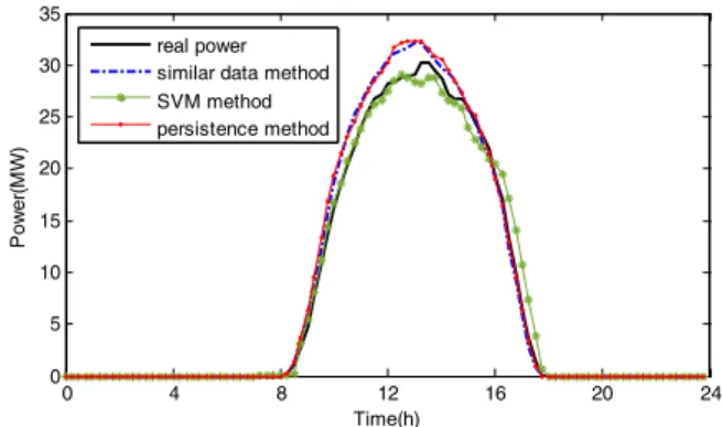
Fig.1 shows the prediction curves of individual forecasting models for January 12, 2013. Fig. 2 shows the relative forecasting errors of different individual models for January 12, 2013. The results show that these models have the ability to track the general trend of the actual output power.
0 4 8 12 16 20 24 0 5 10 15 20 25 30 35 Time(h) Po w e r( MW ) real power similar data method SVM method persistence method
Fig. 1 PV power forecasting results of individual methods ( data collected on 12/1/2013, sunny day)
Fig.2 Relative forecasting errors of individual models ( data collected on 12/1/2013, sunny day) 0 4 8 12 16 20 24 0 2 4 6 8 10 12 Time(h) R e la ti ve e rr o r( % )
similar data method SVM method persistence method
III. COMBINATION PREDICTION MODEL BASED ON ROUGH SET THEORY
A. The Formulation of Combination Forecasting
Combination forecasting tries to put the different forecast models together and utilizes the information of all kinds of forecasting methods to get combination forecasting model. Combination forecasting is an effective way to improve prediction accuracy by combination weights of single forecasting models. Combination forecasting model can be defined as: 1 n i i i P w P = =
(10)Where Pi is forecasting power of i single model, wi is
combination weight of single forecasting model.
B. Rough Set Theory
Rough set theory, proposed by Pawlak in 1982, is a theory used to study information systems characterized by inexact, uncertain or vague information [20],[21]. One advantage is that rough set theory does not need any preliminary or additional information about data. Because it is an effective tool with vast potential for knowledge acquisition and inference, rough set theory has been widely investigated in the field of data mining, decision-making analysis and pattern recognition.
Define a data set, called an information. S is an information system:
{
, , ,}
S= U A V f (11) Where U=
{
x x1, 2,,xn}
is a finite, nonempty sets calledthe universe. A=C∪D is called the set of attributes, C and D
are sets of condition and decision attributes, respectively.
a
V = ∪V is the set of attribute values. With every attribute
A
α∈ , a set Vais associated, of its values, called the domain
of a. :f U×A→V is called information system. If in an information system are represented two classes of attributes, condition and decision attributes, then the system will be called a decision system. Decision system can be described as a decision table. Any decision table induces a set of “if ... then” decision rules. Suppose C1∈C is a condition attribute, the dependency degree of C1 to decision attributes D is defined as:
( )
1( )
1 C C POS D D U γ = (12) Where 1( ) CPOS D is called C -positve region of D,
U denotes all elements of U.
For a decision system, every condition attribute has different degree of the dependency to decision attribute D. In the rough set theory, the significance degree of condition attribute can be measured by classification characteristic of
decision system reducing this condition attribute. The significance degree of condition attribute is defines as:
(
1, ;)
C( )
C C1( )
sig C C D =γ D −γ − D (13)
1 ( , C; D)
sig C is bigger, the effect of condition attribute
1
C for decision is more important. Vice versa. If condition attribute C1 has effect on decision system weakly,
1 ( , C; D)
sig C is smaller, which mean that C1 is insignificance
for making decision.
C. Combination Forecasting Model Based on Rough Model
Rough set theory does not need any preliminary information about data. A significance degree of condition attribute to making decision attribute can be calculated in the rough set theory. The key problem of combination forecasting is how to obtain the combined weight values properly to improve the prediction precision effectively. This paper proposes that combination weight of single forecasting model is determined by rough set based on the significance degree of condition attribute.
The steps of using rough set model to evaluate weighting coefficients of combination predicted model is described as follows:
1) Construct decision table. Using rough set to obtain combination weight, a decision table should be built firstly. Every single forecasting model is defines as condition attribute,
1 2 { , , n}
C= C C C , (iCi =1, 2,n). The PV output power is selected as decision attributeD. Suppose that xtis the element
of universe U , xt ={C1,t,C2,t,Cn t,;Dt}, whereCi t, and Dt
are forecasting power of i single forecasting model and real output power of PV at t instant, respectively.
2) Decision discretization. Because rough set only processes discrete information, the decision table should be discretized. Average interval in the region is adopted to discretize. From the minimum value to maximum value of output power of PV, it is classified as k interval averagely.
3) Calculate the significance degree of condition attribute for single forecasting model.
Taken the single forecasting model as condition attribute, calculate the significance degree of condition attribute for single forecasting model individually by following as (14):
(
, ;)
( )
( )
i
i C C C
sig C C D =γ D −γ − D (14)
4) Calculate the combination weight by following as (15).
(
)
(
)
1 , ; , ; i i n i i sig C C D sig C C D ω = =
(15)5) Evaluate the forecasting power of combination model. Utilizing the combination weight, the forecasting power of combination model can be obtained according to (16).
1 n i i i P
ω
P = =
(16)Where P is forecasting power of combination, Pi is power
of single forecasting model.
D. Simulation Results of Rough Set Combination Prediction
Model
Following the step of combination prediction method based on rough set, we established a combination prediction model and use it to forecast the PV output power of the same PV power plant for January 12, 2013. We obtained the weight coefficients of individual predicted models by rough set and they are listed in Table I.
TABLE I WEIGHT COEFFICIENTS OF COMBINATION MODEL
w1(persistence) w2(SVM) w3(Similar Data)
0.20 0.70 0.10
Fig.3 shows the prediction curve of rough set combination prediction model for January 12, 2013. Fig. 4 shows the relative forecasting errors of rough set weight combination prediction for January 12, 2013. The result shows that the prediction accuracy of rough set combination prediction model is higher than each individual prediction model mentioned above. The RMSE of this method is 2.03%.
0 4 8 12 16 20 24 0 5 10 15 20 25 30 35 Time(h) Po w e r( MW ) real power rough set method
Fig. 3 PV power forecasting results of rough set weight combination prediction method (data collected on 12/1/2013, sunny day)
Fig.4 Relative forecasting errors of rough set combination prediction method (data collected on 12/1/2013, sunny day)
IV. COMPARISON BETWEEN COMBINATION MODEL AND INDIVIDUAL MODELS
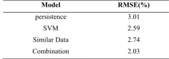
Table II compares the RMSE error for January 12, 2013 caused by of combination forecasting model and individual forecasting models. The RMSE error of rough set combination forecasting model is smaller than individual forecasting models. It indicates that rough set combination forecasting utilities the information of every model and can obviously reduce forecasting error. Rough set combination forecasting model has high forecast accuracy.
TABLE II ERRORS OF DIFFERENT FORECASTING METHODS OF JANUARY 12, 2013, SUNNY DAY Model RMSE(%) persistence 3.01 SVM 2.59 Similar Data 2.74 Combination 2.03
Because January 12, 2013 was a sunny day, it is easy to obtain the high accuracy for prediction method. In order to verify the applicability of rough set combination forecasting model to various weather types, a cloudy day October 23, 2012 is chosen to verify the prediction accuracy of combination forecasting model. The combination weights obtained for October 23, 2012, which are w1=0.75(persistence), w2=0.15
(SVM), w3=0.10 (Similar Data).
TABLE III WEIGHT COEFFICIENTS OF COMBINATION MODEL OF OCTOBER 23,2012, CLOUDY DAY
w1(persistence) w2(SVM) w3(Similar Data)
0.75 0.15 0.10
Fig.5 shows the prediction curves of individual forecasting models for October 23, 2012. Fig.5 indicates that these single models prediction accuracy are lower on a cloudy day. The RMSE of persistence method, SVM and similar data method are 8.14%, 8.12%, and 8.19%. 0 4 8 12 16 20 24 0 2 4 6 8 10 12 14 16 Time(h) Po w e r( MW ) real power similar data method SVM method persistence method
Fig. 5 PV power forecasting results of individual methods (data collected on 23/10/2012, cloudy day)
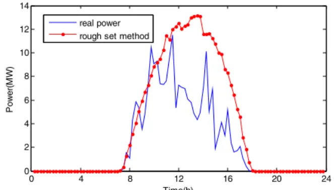
Fig.6 shows the prediction curve of rough set combination prediction model for October 23, 2012. And the RMSE of this method is 7.38%. The result shows that the prediction accuracy of rough set combination prediction model is higher than each individual prediction model mentioned above.
0 4 8 12 16 20 24 0 2 4 6 8 10 12 Time(h) R e la ti v e e rro r(% )
0 4 8 12 16 20 24 0 2 4 6 8 10 12 14 Time(h) Po w e r( MW ) real power rough set method
Fig.6 PV power forecasting results of rough set combination prediction method (data collected on 23/10/2012, cloudy day)
Table IV compares the RMSE and the maximal relative errors of combination forecasting model and individual forecasting models for October 23, 2012.
TABLE IV ERRORS OF DIFFERENT FORECASTING METHODS OF OCTOBER 23RD, 2012, CLOUDY DAY Model RMSE(%) persistence 8.14 SVM 8.12 Similar Data 8.19 Combination 7.38
Comparing data in Table II, and Table IV, it can be noticed that rough set combination forecasting model reduces the predicted error and improve predicted accuracy in sunny day and cloudy day. This indicates that rough set combination forecasting model is adaptive to prediction for different weather types.
V. CONCLUSIONS
In this work, a new method of PV power forecasting is investigated. Three prediction models are firstly used for PV power prediction including the persistence method, the SVM model and the similar data method. A combination prediction model is then proposed to integrate the three different PV forecasting models through objective weightings designed by a rough set method. This proposed combination prediction model has the strength over each individual forecasting model in that the prediction error due to each individual method is compensated through a proper combination of several methods. The simulation results demonstrate that the combination forecasting method is able to improve the prediction accuracy effectively and also the prediction result is more robust for different weather conditions than any of the single forecasting methods.
REFERENCES
[1] G. S. Kinsey, A. Nayak, M. Liu, V. Garboushian, and S. Beach, “Increasing Power and Energy in Amonix Solar Power Plants,” IEEE J. Photovoltaics, vol. 1, no. 2, pp. 3–4, 2011.
[2] C. Paoli, C. Voyant, M. Muselli, and M. L. Nivet, “Forecasting of preprocessed daily solar radiation time series using neural networks,” Sol. Energy, vol. 84, no. 12, pp. 2146–2160, 2010.
[3] E. Lorenz, J. Hurka, D. Heinemann, and H. G. Beyer, “Irradiance forecasting for the power prediction of grid-connected photovoltaic systems,” IEEE J. Sel. Top. Appl. Earth Obs. Remote Sens., vol. 2, no. 1, pp. 2–10, 2009.
[4] L. A. Fernandez-Jimenez, A. Mu??oz-Jimenez, A. Falces, M. Mendoza-Villena, E. Garcia-Garrido, P. M. Lara-Santillan, E. Zorzano-Alba, and P. J. Zorzano-Santamaria, “Short-term power forecasting system for photovoltaic plants,” Renew. Energy, vol. 44, pp. 311–317, 2012.
[5] A. Yona, T. Senjyu, A. Y. Saber, T. Funabashi, H. Sekine, and C. H. Kim, “Application of neural network to one-day-ahead 24 hours generating power forecasting for photovoltaic system,” 2007 Int. Conf. Intell. Syst. Appl. to Power Syst. ISAP, 2007.
[6] P. Bacher, H. Madsen, and H. A. Nielsen, “Online short-term solar power forecasting,” Sol. Energy, vol. 83, no. 10, pp. 1772–1783, 2009. [7] Y. Li, Y. Su, and L. Shu, “An ARMAX model for forecasting the
power output of a grid connected photovoltaic system,” Renew. Energy, vol. 66, pp. 78–89, 2014.
[8] Z. Wang, S. Su, and S. Zhang, “The application of photovoltaic power prediction technology,” 2011 Int. Conf. Electron. Commun. Control. ICECC 2011 - Proc., pp. 2343–2346, 2011.
[9] J.-L. Chen, H.-B. Liu, W. Wu, and D.-T. Xie, “Estimation of monthly solar radiation from measured temperatures using support vector machines – A case study,” Renew. Energy, vol. 36, no. 1, pp. 413–420, 2011.
[10] C. Tao, D. Shanxu, and C. Changsong, “Forecasting power output for grid-connected photovoltaic power system without using solar radiation measurement,” 2nd IEEE Int. Symp. Power Electron. Distrib. Gener. Syst., pp. 773–777, 2010.
[11] N. Sharma, P. Sharma, D. Irwin, and P. Shenoy, “Predicting solar generation from weather forecasts using machine learning,” Smart Grid Commun. (SmartGridComm), 2011 IEEE Int. Conf., pp. 528–533, 2011.
[12] M. Malvoni, M. G. De Giorgi, and P. M. Congedo, “Photovoltaic power forecasting using statistical methods: impact of weather data,” IET Sci. Meas. Technol., vol. 8, no. January, pp. 90–97, 2014.
[13] C. E. Borges, Y. K. Penya, and I. Fernandez, “Evaluating Combined Load Forecasting in Large Power Systems and Smart Grids,” IEEE Trans. Ind. Informatics, vol. 9, no. 3, pp. 1570–1577, 2013.
[14] J. Che, J. Wang, and G. Wang, “An adaptive fuzzy combination model based on self-organizing map and support vector regression for electric load forecasting,” Energy, vol. 37, no. 1, pp. 657–664, 2012.
[15] L. Li, C. Mu, S. Ding, Z. Wang, R. Mo, and Y. Song, “A Robust Weighted Combination Forecasting Method Based on Forecast Model Filtering and Adaptive Variable Weight Determination,” Energies, vol. 9, no. 1, p. 20, 2015.
[16] B. S. Ahn, S. S. Cho, and C. Y. Kim, “The integrated methodology of rough set theory and artificial neural network for business failure prediction,” Expert Syst. Appl., vol. 18, no. 2, pp. 65–74, 2000. [17] J. H. Cheng, H. P. Chen, and Y. M. Lin, “A hybrid forecast marketing
timing model based on probabilistic neural network, rough set and C4.5,” Expert Syst. Appl., vol. 37, no. 3, pp. 1814–1820, 2010. [18] K. Y. Huang and C. J. Jane, “A hybrid model for stock market
forecasting and portfolio selection based on ARX, grey system and RS theories,” Expert Syst. Appl., vol. 36, no. 3 PART 1, pp. 5387–5392, 2009.
[19] V. N. Vapnik, Statistical Learning Theory. New York.: Wiley, ch. 2, pp. 375-400,1998.
[20] Z. Pawlak, “Rough sets,” Int. J. Comput. Inf. Sci., vol. 11, no. 5, pp. 341–356, 1982.
[21] Z. Pawlak, “Rough Set Theory and Its Applications To Data Analysis,” Cybern. Syst. An Int. J., vol. 29, no. April 2015, pp. 661–688, 1998. .