Data-driven reduction strategies for Bayesian inverse problems

(1)

DISCLAIMER:

This document does not meet

the

current format guidelines

of

the

Graduate School at

The University of Texas at Austin.

It has been published for

(2)

Copyright by

Ellen Brooke Le 2018

(3)

The Dissertation Committee for Ellen Brooke Le

certifies that this is the approved version of the following dissertation:

Data-Driven Reduction Strategies for Bayesian

Inverse Problems

Committee:

Tan Bui-Thanh, Co-Supervisor Quoc P. Nguyen, Co-Supervisor Omar Ghattas

J. Tinsley Oden Rachel Ward

(4)

Data-Driven Reduction Strategies for Bayesian

Inverse Problems

by

Ellen Brooke Le

DISSERTATION

Presented to the Faculty of the Graduate School of The University of Texas at Austin

in Partial Fulfillment of the Requirements

for the Degree of

DOCTOR OF PHILOSOPHY

THE UNIVERSITY OF TEXAS AT AUSTIN May 2018

(5)

(6)

What the mind doesn’t understand, it worships or fears.

Alice Walker

I can see that without being excited, mathematics can look pointless and cold.

Maryam Mirzakhani,1977-2017

Free will, though it makes evil possible, also makes possible any love or goodness or joy worth having.

(7)

Acknowledgments

I am extremely grateful to my ICES supervisor Tan Bui-Thanh, for his support, sharp scientific guidance, and the monumental effort he put into training me since my first year at UT. Under Tan’s direction I have grown spiritually and intellectually, far more than I imag-ined I would during five years (—did I even learn anything in undergrad?). With each year of this PhD, I felt exponentially greater depth of understanding and confidence in my capacity to do creative, valuable work—and if only because, while reading old material or code I had written the previous year, I’d think something like, ‘well, this is not technically wrong, but I really had no idea! [to the degree that I havesomeidea now]’. It is a blessing to have this feeling. I am grateful that Tan kept high standards and never gave up on me. I am also grateful to have Tan not only as an academic role model, but as a personal one. People who don’t know him might wrongly perceive him as a singularly-minded workaholic researcher, who must be making trade-offs somewhere else in life, but they do not realize that he is an excellent and caring instructor, a devoted husband and father, a talented gardener and karaoke singer, and can do more pull-ups than our entire research group combined (sadly). His achievements are a testament to approaching all of life with energy, conscientiousness, and passion.

I am also indebted to my PGE co-advisor Quoc P. Nguyen for his support, patience, and generosity, and for bringing me up to speed quickly in the world of petroleum and subsurface transport, which was a completely new domain for me. Going on the job market this past year was not easy, but I strongly believe that being able to discuss real world inverse problems in depth, in addition to research, made my application stand out—and for this I am grateful to Dr. Nguyen. Both my advisors were instrumental in providing my uncommon graduate school experience—how many people can say they went to Europe, Australia, and

(8)

Canada for the first time during their PhD, to present their research? I recognize this is unusual, and thank both for their generosity and trust in my presentation skills.

I wish to express gratitude to my committee, for the content and shape of this disser-tation. With their assistance it has become something I can be proud of. I thank especially Professor J. Tinsley Oden, the person most responsible for developing ICES into the dream team of computational scientists that it is today—the veritable “New York Yankees of re-searchers,” as Benj likes to say. At the time of writing, ICES is the number one ranked program in the world, thanks to Prof. Oden’s remarkable direction and pioneering vision. I have already benefited so much from Prof. Oden’s work, so I am humbled, honored, and slightly embarrassed by the fact that he read my thesis word for word with a highlighter and managed to find errors that many (smart!) people and passes could not. I acknowledge deep gratitude for his time and dedication to excellence.

I am grateful to my committee members Omar Ghattas and Rachel Ward, who are both superstars in their fields, for taking the time to really understand the methods here, in order to offer their unparalleled insights that shaped the final dissertation for the better. Thank you.

Many thanks to my collaborators: Aaron Myers, Dan O’Malley, Monty Vesselinov, Youzou Lin, and Vishwas Rao, for support, helping me to develop ideas, allowing me to experience the storied lab life at Los Alamos, and to have fun while doing research. Regarding Los Alamos, I thank Dr. Bill Press for turning me into a Bayesian for life, and helping me find last minute housing both for me and my cat. I am grateful to ICES for the generous CSEM Fellowship and TACC for the computing resources and timely help. I thank SIAM, AAAS, and the Sac Bee editors for my summer at the newsdesk, which I did not realize would help so much with writing this dissertation. Heartfelt thanks to my cohort and mentors from EDGE 2011, especially Ami Radunskaya (Dr. Rad) and Rhonda Hughes, for showing that you can be a world-class mathematician and still a genuine heart-on-your-sleeve person who

(9)

believes in everyone. You don’t know how much strength and inspiration you all gave me! I reach back to that summer so much when I feel like quitting, which has been often. Dr. Caitlin McClune of the University Writing Center has been especially vital in craziness of my final writing days—thank you. I am indebted to the PCL library staff for the silent study where I wrote the majority of this dissertation.

For nourishing my humanity during these past few months of self-imposed isolation in a windowless room, I am lucky to have amazing friends and family. They managed to reach me with everything from texts of motivating gifs to actual gifts (what!). Thank you to my mother and father for overcoming so much, teaching me to love math, and now for the continual reminders to eat vegetables and just be happy. Thank you to my first role model, Maj. Viet Le, for helping me to believe that greatness is in my blood, and trying your best to get me to be good at sports. It made school easier. I thank my dear, accomplished sister Emily Le, my life coach—no doubt I got through many tough times with her tough no-nonsense talk!

I could have never made it without the support from my sweet, intelligent, and wonderful friends for life: Dee Dee White, Hannah Frederick, Jessica Le, Isabelle Atkinson, Sarah Parker, Stacey Burke, Madelyn DeYoung—you guys will actually change the world. I look up to you! Lastly I thank my fiance Benj Wagman, to whom this this thesis is dedicated, for being there one hundred and ten percent for me, throughout all the ups and downs of the past five years, and being the only person to laugh at my jokes. Over the past few months, you have sweetly accepted my descent into madness, and selflessly offered all the support one can offer, even though you have had your own dissertation to contend with. A PhD does not guarantee a good career or life, but it is an important step for both of us. I am grateful for your trust, and feel nothing other than happiness to have you with me on this uncertain journey. I look forward to spending more time with you.

(10)

Data-Driven Reduction Strategies for Bayesian

Inverse Problems

Publication No.

Ellen Brooke Le, Ph.D.

The University of Texas at Austin, 2018 Co-Supervisors: Tan Bui-Thanh

Quoc P. Nguyen

A persistent central challenge in computational science and engineering (CSE), with both national and global security implications, is the efficient solution of large-scale Bayesian inverse problems. These problems range from estimating material parameters in subsurface simulations to estimating phenomenological parameters in climate models. Despite recent progress, our ability to quantify uncertainties and solve large-scale inverse problems lags well behind our ability to develop the governing forward simulations.

Inverse problems present unique computational challenges that are only magnified as we include larger observational data sets and demand higher-resolution parameter estimates. Even with the current state-of-the-art, solving deterministic large-scale inverse problems is prohibitively expensive. Large-scale uncertainty quantification (UQ), cast in the Bayesian inversion framework, is thus rendered intractable. To conquer these challenges, new methods that target the root causes of computational complexity are needed.

In this dissertation, we propose data-driven strategies for overcoming this “curse of di-mensionality.” First, we address the computational complexity induced in large-scale inverse problems by high-dimensional observational data. We propose a randomized misfit approach

(11)

(RMA), which uses random projections—quasi-orthogonal, information-preserving transfor-mations—to map the high-dimensional data-misfit vector to a low-dimensional space. We provide the first theoretical explanation for why randomized misfit methods are successful in practice with a small reduced data-misfit dimension (n =O(1)).

Next, we develop the randomized geostatistical approach (RGA) for Bayesian sub-surface inverse problems with high-dimensional data. We show that the RGA is able to resolve transient groundwater inverse problems with noisy observed data dimensions up to

107, whereas a comparison method fails due to out-of-memory errors.

Finally, we address the solution of Bayesian inverse problems with spatially localized data. The motivation is CSE applications that would gain from high-fidelity estimation over a smaller data-local domain, versus expensive and uncertain estimation over the full simulation domain. We propose several truncated domain inversion methods using domain decomposition theory to build model-informed artificial boundary conditions. Numerical investigations of MAP estimation and sampling demonstrate improved fidelity and fewer partial differential equation (PDE) solves with our truncated methods.

(12)

Chapter 1

Introduction

This dissertation proposes new data-driven methods towards making state-of-the-art Bayesian inversion and uncertainty quantification (UQ) tractable for large-scale problems: problems of data assimilation and statistical inference, governed by computationally ex-pensive PDE-based models and high-dimensional input parameters. Here, high-dimensional means the dimension is in the hundreds, thousands, or millions. The high dimensionality is typically due to discretization of a spatially distributed heterogeneous parameter in a two-or three-(space)-dimensional model. Computationally expensive means that a single ftwo-orward simulation takes hours or days to finish, even when optimized for distributed computing on leadership-class supercomputers.

Important large-scale inverse problems exist in numerous different areas of compu-tational science and engineering (CSE). As just a few examples of active areas of research, these include:

• Ice sheet modeling: Estimating the phenomenological basal sliding parameter in Antarc-tic ice sheet models, using remote sensing observations of surface ice flow.

• Bioremediation: Estimating the future spatial distribution of the full chromium plume endangering the Los Alamos, New Mexico water table, using concentration and pro-duction data from current localized mitigation efforts at wells.

• Energy independence: Estimating the current spatial distribution of residual oil in a mature West Texas reservoir, using production history data and concentration history

(16)

from a partitioning interwell tracer test. This information is critical for thorough risk-assessment of expensive (upwards of several million USD [133]) enhanced oil recovery projects.

• Earth system modeling: Estimating the climate response to regional and cloud-scale input parameters, to advance development of exascale-ready high-resolution simula-tions of clouds in climate models. This could reduce the largest source of uncertainty in predictions of future climate.

The methods proposed in this dissertation are designed to apply to all of the inverse problems above, as well as others. Fortunately, these different problems possess similar math-ematical challenges. They are ill-posed, and governed by computationally expensive-to-solve partial differential equation (PDE) models, heterogeneous high-dimensional parameters, and increasingly, large amounts of observational data.

1.1

Needs and challenges in solving large-scale Bayesian inverse

problems

Despite remarkable advancements in the past two decades, current methods for solving Bayesian inverse problems are limited to problems of modest computational complexity and input parameter dimension [2, 4, 25, 59, 124]. Standard Bayesian inversion methods such as Markov Chain Monte Carlo (MCMC) require hundreds of thousands or millions of simulations to converge. Thus, they are prohibitive for large-scale models.

Solving the Bayesian inverse problem is a straightforward approach to uncertainty quantification. The uncertainty in the unknown input parameters is completely described by the posterior probability—the solution of the Bayesian inverse problem. The uncertainty in predictions and quantities of interest is then quantified by propagating the posterior input parameter statistics through the forward model. The difficulty is the acute

(17)

compu-tational complexity of solving the Bayesian inverse problems with large-scale models and high-dimensional parameter spaces.

Yet, the need to quantify and reduce the uncertainty in our computational models is urgent. Scientists and policy-makers across the spectrum agree increasingly that predictions must be equipped with quantified uncertainty in order to be of pragmatic, actionable use for decision-makers and CSE stakeholders. For example, despite the recent change in ad-ministration, the term “uncertainty” five times in the FY 2018 U.S. Department of Energy (DOE) Budget Request brief—the same number of times that it appeared in the FY 2017 brief (compare this to only one appearance in the FY 2016 brief).

1.1.1 Existing strategies and limitations

Several approaches exist for addressing the computational challenge posed by the large-scale Bayesian inverse problems of interest. The approaches are not necessarily sepa-rate, and include:

• Attack the forward solve (simulation) computational cost: Make PDE solvers faster or develop cheaper surrogate models.

• Attack the Bayesian UQ method: Develop viable alternative sampling approaches to standard approaches. Standard vanilla MCMC, Latin Hypercube Sampling (LHS), and polynomial chaos expansion-based sampling are not viable for the large-scale inverse problems of interest due to the computational cost required for convergence to the posterior probability [20,100]. Or, develop methods to accelerate MCMC convergence while minimizing the number of model evaluations [38].

• Use intrusive or embedded UQ methods: The majority of available UQ tools treat the parameter-to-observable map as a black box. Intrusive or embedded UQ methods, on the other hand, require access to gradients of the underlying forward operator,

(18)

motivated by the fact that the output of PDE models is locally smooth. Recently developed intrusive methods exploit the mathematical properties of the parameter-to-observable operator and have been successfully applied to inverse UQ problems with parameter dimensions in the millions [25, 65].

• Develop targeted reduction strategies: Identify mathematical structure components that have the largest impact on the computational cost estimate for solving the Bayesian inverse problem and replace them with goal-oriented, reduced order components—this category includes reduced order modeling approaches, but is broader.

The method development approach in this dissertation is best characterized by the last bullet point.

1.1.2 Motivation for developing data-driven reduction strategies

Only compounding difficulties is the demand to resolve Bayesian inverse problems with larger discretized state, parameter, and data dimensions. This is in part due to the big data challenge that is rapidly changing the field of computational science and engineering (CSE), as result of improved measurement technology and ability to store large volumes of data [124]. Thus, another emerging challenge in computational science and engineering is the solution of large-scale statistical inverse problems governed by PDEs that involve large amounts of observational data. Alternatively, although the data may be high-dimensional, it is often still located in and informative for a spatially-concentrated subregion of the full model domain. The data-informed subregion is a lower-dimensional subset of the high-dimensional parameter and state spaces. New inversion methods that target and exploit these emerging data paradigms are needed.

(19)

1.2

Dissertation goal

The goal of Bayesian inverse problems is to infer knowledge from data. Progress towards this goal in many large-scale problems is impeded by the computational challenges outlined in section 1.1. Despite the promise of big data and technological advances in data collection and measurement, computational challenges persist, and new strategies are needed [124]. The goal of this dissertation is to develop new, data-driven strategies for efficiently and effectively solving large-scale Bayesian inverse problems—and therefore make the extraction of knowledge from data both timely and tractable.

1.3

Dissertation contributions

The main contributions of this dissertation towards the above stated goal are a method for reducing the computational impact of big data, and a method for reducing the complexity induced by high-dimensional parameter and state spaces in problems with spatially local data. Both reduction strategies are theoretically justified, using large deviation theory and domain decomposition theory, respectively.

Specifically, a theoretical contribution of this dissertation is the first guarantee of validity for the deterministic solution obtained with a randomized misfit, with a small reduced dimension. This provides an explanation for the observed surprising quality of solutions when using a randomized misfit function with a small reduced dimension, which has been noted in other randomized misfit methods. The efficacy of the randomized misfit approach in this dissertation is shown to be the result of the interplay between Morozov’s discrepancy principle and random projection theory. As will be shown, the data error and ill-posedness inherent in inverse problems is essential to the success of random projections.

This key contribution is due to the use of large deviation theory to arrive at a practical, statistical characterization of solution convergence. Large deviation techniques form the

(20)

basis of random projection theory and analysis of other effective randomized dimension reduction algorithms (e.g. randomized SVD). Here, it is used to show the RMA exploits a “concentration of measure” phenomenon for high-dimensional data. It is shown that for a certain class of distributions, the tail probability of a sample average of misfit estimators decays exponentially, with a rate parameterized by the sample size. This statement is turned into a probabilistic bound on the randomized cost for a fixed data misfit dimension .

Another novel contribution of the approach presented in this dissertation is that it permits the use of many random projections in the literature.

Additionally, from the stochastic formulation of the misfit, a different version of the Johnson-Lindenstrauss embedding theorem [42,64,96] is shown. This leads to an insight into why the reduced misfit dimensionnisO(ε−2), whereεis the relative error of the randomized cost function.

The dissertation also demonstrates and shows comparable results for a practical RMA extension to geoscience inverse problems with big geostatistical data [88], called the ran-domized geostatistical approach (RGA). It extends the widely used Bayesian geostatistical approach (GA) [74], and its extension called the principal component geostatistical approach (PCGA) [73, 84].

The GA is known to be limited to only moderate size problems [73, 84]. Although the PCGA, a randomized approximation of the GA, extends the GA to solve problems with problems with high-dimensional parameter spaces (O(105₎_{− O}₍₁₀7₎_{), it is limited to}

moder-atedata dimensions ( (O(104₎) [73,84]. The RGA extends the GA to inverse problems with

problems with high-dimensional (O(105₎_{− O}₍₁₀7₎) parameter spaces _and high-dimensional

data. The analysis and results presented in this dissertation demonstrate comparable pa-rameter estimation and convergence results as the PCGA in a groundwater inverse problem. However the RGA experiments show a 31 times speed-up. Numerical results in this disserta-tion also show the RGA is able to solve geostatistical inverse problems with up to observed

(21)

data dimensions of up to O(107₎_{, whereas PCGA fails due to insufficient memory.}

This dissertation also contributes the development of several truncated domain in-version strategies and methods. These methods directly reduce the problematic high-dimen-sionality of the parameter and state domain by shrinking the model domain, and only in-verting for an informed subregion of the model. They exploit an insight that observed data, which is often located in a smaller region than the full model domain, is spatially-limited in parameter information. Using the uncertainty estimation at the maximum a posteriori (MAP) point, and building on domain-decomposition methods and work that uses Dirchlet-to-Neumann (DtN) maps to build mathematically-justified artificial boundary conditions, different model-constrained and low-offline-cost methods are investigated. Results with a distributed thermal conductivity inverse problem demonstrate that truncated inversion can be more efficient and effective. An idea is supported with results from both MAP esti-mation and sampling experiments, that fidelity in MAP point estiesti-mation results could be improved and the posterior can be easier to characterize, by removing high uncertainty re-gions from the inversion domain. That is, the strategy is effective not only because it reduces high-dimensional state and parameter space, but also because it fundamentally changes the full domain posterior and problem. Given the same amount of computational resources, this means more distributed parameter information can be extracted from the observed data, and therefore fulfills the dissertation goal towards making large-scale Bayesian inversion timely and tractable.

1.4

Dissertation outline

The following chapters develop different reduction strategies for reducing the com-plexity of solving large-scale Bayesian inverse problems.

(22)

Specifically, each method exploits one of two data paradigms that are commonly observed in the large-scale setting: either the data is high-dimensional, or the data is located in a smaller subregion relative to the full model domain, and contains spatially-limited information about the unknown distributed parameter.

Chapter 3 introduces the randomized misfit approach (RMA) a targeted application of a machine learning tool called a random projection, to reduce the high computational cost of solving big data, high-fidelity physics-based inverse and its analysis. Section 3.6

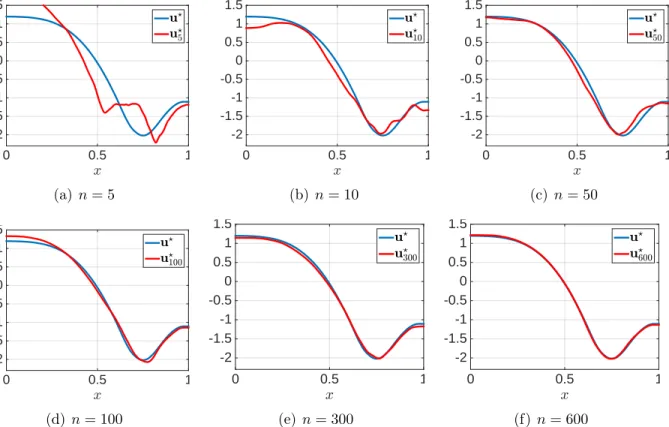
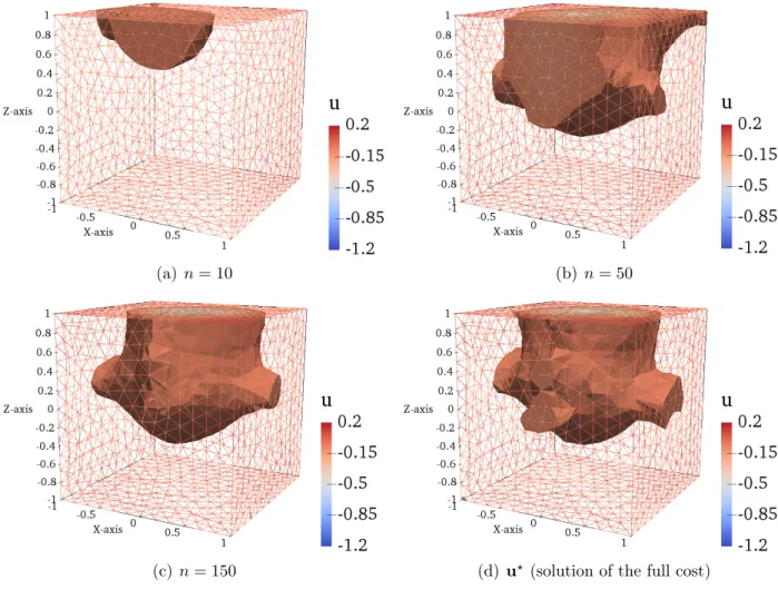
presents the theoretical analysis for the randomized misfit approach by deriving the large deviation bounds on the objective function error for a broad class of distributions. The reduced misfit dimension is shown to be independent of the original data dimension. This derivation leads to a different proof of a variant of the celebrated Johnson-Lindenstrauss embedding theorem. A statistical Morozov’s discrepancy principle, Theorem 2 shows that the effective reduced misfit dimension is also bounded below by the noise in the problem. Therefore, the RMA solution is a guaranteed solution for the original problem with a high user-defined probability. The reduced computational cost in problems with high-dimensional data is assessed in subsection 3.6.3. Section 3.7 summarizes numerical experiments on a model inverse heat conduction problem in one-, two-, and three spatial-dimensions. The RMA solution with different distributions is compared to the solution of the full problem. Numerical support for Theorem 2 is also investigated.

Chapter 4 introduces and motivates the RGA, first briefly introducing the Bayesian geostatistical approach (GA) [74], a widely used geostatistical inversion method, and its extension to large-scale problems with high-dimensional parameter spaces [84] called the principal component geostatistical approach (PCGA) [84].

In section4.6, it is shown that the RGA can be more effective than the PCGA method when the number of observations is large. In section 4.7, numerical tests of the RGA against PCGA with a big data transient groundwater inverse problem are given.

(23)

Chapter 5examines domain-decomposition methods for large-scale inverse problems, and both model constrained and low-offline cost methods are developed. Numerical results demonstrate higher-fidelity inversion and UQ results with improved computational efficiency by truncating the problem domain.

Chapter6briefly discusses ongoing extensions of the methods presented in Chapters3

(24)

Chapter 2

Inverse problem formulation

This dissertation develops methods towards the efficient solution of large-scale Bayesian inverse problems, which are briefly overviewed in Chapter 1, along with current challenges and existing strategies. The aim of this preliminary chapter is to introduce the mathemat-ical formulation for the abstract Bayesian inverse problem of interest, and thus make the objectives of the dissertation methods concrete. The general notation will remain the same throughout this dissertation, with only a few necessary modifications for different methods and applications. This chapter also introduces a nonlinear inverse problem, the estimation of a distributed coefficient in a linear elliptic PDE. This model problem is the basis for each of the driving examples presented in this dissertation, with method-specific extensions.

2.1

The objective of the inverse problem

The main goal of an inverse problem is to infer an unknown inputparameter u using indirect observed data d. The parameter cannot by observed directly, for reasons that vary and depend on the application. In PDE-constrained inverse problems, a system of PDEs governs the relationship between the unknown u and observed noisy d.

The methods developed in this dissertation address computationally prohibitive-to-solve inverse problems—specifically, problems that are large-scale and have spatially-distributed unknown parameters, which are high-dimensional when discretized. Here, large-scale means that a single forward solve can take minutes to hours, even on supercomputers.

(25)

Assuming a common Gaussian additive noise model for the observed data:

dj =w(xj;u) +ηj, j = 1, . . . , N, (2.1)

the inverse problem objective is to reconstruct the distributed parameter u given N data points dj. For a given u, a set of discretized states w(xj;u) is obtained by evaluating an expensive-to-solve forward model (generally a system of PDEs), and then applying a linear observation operator to match the data locations. The location of an observational data point in an open and bounded spatial domainΩis denoted byxj, andηj is Gaussian random noise with mean 0 and variance σ2

noise.

Concatenating the observations, (2.1) can be rewritten as

d=F(u) +η, η∼ N(0,Γnoise) (2.2) where

Γnoise:=σnoise2 IN (2.3)

and F(u) := [w(x1;u), . . . ,w(xN;u)]

> _{is the parameter-to-observable map. Thus the}

model forward problem is to solve (2.4)for the unknown distributed temperatureu, given a known distributed log conductivity u.

The model inverse problem is to reconstruct the distributed log conductivityu, given noisy observed measurements d of temperature won Ω.

The parameter-to-observable map F(u) encodes a single, computationally-expensive

solve of the forward model, represented by(2.4)in the given model inverse problem, followed by extraction to the data locations. It is generally a nonlinear map, even when the PDE system is linear in the state [25], as will be the case with the model forward PDE(2.4) used throughout this dissertation.

(26)

2.2

Forward model

In formulating an inverse problem, the forward problemis the well-posed problem of obtaining the state w (the forward solution), given a parameter u.

The forward problem is governed by the forward (physics) model which is generally a system of PDEs.

2.2.1 Model problem: Elliptic forward PDE

The model problem for initial development and testing of methods in this dissertation is the estimation of a distributed coefficient in an elliptic partial differential equation. This Poisson-type problem arises in various inverse applications, such as the steady-state thermal conductivity or groundwater problem, or in finding a membrane with a given spatially-varying stiffness.

For concreteness, consider the forward heat conduction problem on an open bounded domainΩ, governed by

−∇ ·(eu∇w) = f(u) in Ω

−eu_∇w_·_n₌_Bi_w _on_∂_ΩBi

−eu_∇w_·_n₌₋₁ _on_∂_ΩRHS

(2.4) where the forward state w is the spatially distributed temperature on Ω, the material

co-efficient u is the logarithm of distributed thermal conductivity on Ω, n is the unit out-ward normal on ∂Ω = ∂ΩBi_∪_∂_ΩRHS_{, and Bi is the Biot number. The model domain is} Ω ∈ _Rn_{, n} _{= 2}_,₃_{. Here,} _∂_ΩRHS _{is a portion of the boundary} _∂_Ω _{on which the inflow heat}

flux is 1. The rest of the boundary, ∂ΩBi_{, is assumed to have Robin boundary condition.}

Thus the model forward problem is to solve (2.4) for the unknown distributed tem-perature u, given a known distributed log conductivity u.

The model inverse problem is to reconstruct the distributed log conductivityu, given noisy observed measurements d of temperature won Ω.

(27)

2.3

The deterministic inverse problem

The deterministic inverse problem governed by (2.4) is the problem of estimating a single unknown log conductivity parameter u that could have led to the data d.

Unlike the well-posed forward problem, the inverse problem is generally ill-posed; many different spatially-varying log conductivities u fit the observed data equally well. An intuitive reason is that discrete observations can only contain limited information about an infinite-dimensional parameter. The more complete explanation is that the parameter-to-observable map exhibits rapid spectral decay. This can be numerically observed and has been proven for many practical inverse problems [18, 19, 21].

Therefore, to overcome ill-posedness and solve the deterministic problem, classical inverse problem approaches add a regularization term to the cost functional . The regular-ization can be thought of as adding additional criteria to the original data-misfit minimregular-ization problem, in order to single out one “best” estimate of u.

A standard deterministic Tikhonov approach resolves the ill-conditioning by adding a quadratic term to the cost function, so that the problem may now be formulated as

min u J(u) = 1 2kF(u)−dk 2 Γ−_noise1 + 1 2ku−u0k 2 C−1. (2.5) wherev=Γ 1 2

noise(d−F(u))is the (noise-weighted)data misfit vector, Euclidean norm inRN is denoted by k·k, and ||·||_C−1 = C 1 2·

is the norm weighted by an appropriately chosen

regularization matrix C.

2.4

The Bayesian statistical inverse problem

In this dissertation adopts the framework of theBayesian inverse problem, which seeks a statistical description of all probable parameter fields u consistent with the observations, rather than a single best u.

(28)

That is, the solution of the Bayesian inverse problem is the posterior probability distribution function (pdf) of the unknown parameter, given the observed data.

It requires specification of a likelihood model, which characterizes the probability that the parameter u could have produced the observed data d. It also requires a prior model, which is problem-dependent and represents a subjective belief regarding the distribution of u.

There are other reasons to prefer a Bayesian approach, in addition to obtaining a distribution of probable u that could have led to the data One reason is that Bayesian inversion is a systematic yet flexible, and naturally well-posed framework for integrating sources of parameter information from observational data, physics-information (encoded in the model), and the subjective judgment of domain experts (encoded in the prior). To paraphrase succinctly, Bayesian inverse problems seek to infer knowledge from data.

2.4.1 Bayesian inverse problems and UQ

Another reason is that Bayesian inversion offers uncertainty quantification. That is, the uncertainty in the unknown parameter u is fully described by the posterior probability distribution. The Bayesian posterior probability distribution accounts for the uncertainties in the observations, the forward model, and the prior knowledge, thus completely quantifying the uncertainty in the unknown parameter u.

Note the single point estimate given by the solution to the deterministic inverse problem (2.5) does not account for the uncertainty in the solution.

To keep the discussion short, the presentation of Bayesian inversion here is finite-dimensional (i.e. after a finite element method (FEM) discretization of the parameter space). However, in the numerical results presented in section 3.7 and section 5.5, discretization is performed rigorously following [23, 135]. Please see [26] for elaboration of the infinite-dimensional framework and the subtle mathematical issues related to the proper choices of

(29)

prior and discretization, and [23] for the exact construction used.

The rest of this dissertation refers to u and u and their discretized quantities unless specified (here, the nodal values with a finite element discretization).

Thus, our discretized unknown parameter u is a finite dimensional vector in _RP, where P is the number of FEM mesh points. Since we assume u is spatially heterogeneous overΩ—similar to large-scale inverse problems of interest—this implies we have a sufficiently

high-resolution mesh discretization and therefore P is large. The same mesh is used for the discretized state u∈_RP_.

The additive-noise model (2.2) is used to construct the likelihood pdf which is ex-pressed as

πlike(d|u)∝exp

−1 2 db−Fb(u) 2 . (2.6)

For concreteness of presentation, for Chapter 3 and Chapter 5 it is postulated that the prior is a Gaussian random field with mean u and a covariance operator C. Γprior is the discrete analog of an infinite-dimensional smoothness prior covarianceCprior that is con-structed following [23]. Specifically, C =A−2_{, where} _A _{is a Laplacian-like operator with its}

domain of definition specified by an elliptic PDE, appropriately-chosen boundary conditions, and parameters than can encode spatial correlation and anisotropy information (for specific implementation details see [6, 26]). This choice avoids constructing and inverting a dense covariance matrix and exploits existing fast solvers for elliptic operators. It additionally provides a connection to the Matérn covariance functions used frequently in geostatistics [77, 89,127] and therefore has a scientific justification.

This choice of thisCprioris only to ensure basic sanity criteria (e.g. bounded pointwise variance) and well-posedness of the Bayesian inverse problem under the criteria for a trace-class operator in [135], and to be computationally amenable to large-scale problems. The reader is referred to [23, 135] for further discussion.

(30)

Note that the square root is not known for arbitrary generalized covariance functions common in geostatistical inverse problems. Thus, Chapter4addresses a practical data-driven method amenable for generalized covariance matrices in geostatistical problems.

Thus, given the assumption of a Gaussian prior and the additive noise model (2.2),

RD, the posterior density function (pdf) of u—the solution to the Bayesian inverse

prob-lem—is π(u|d)∝exp −1 2kF(u)−dk 2 Γ−_noise1 − 1 2ku−u0k 2 Γ−_prior1 (2.7) where F(u)∈_RD _{is the parameter-to-observable map and} _Γ

prior is an appropriately chosen prior covariance matrix.

Unfortunately, there are no closed-form expressions for moments of the posterior in general [40]. Despite the choice of Gaussian prior and noise, the posterior probability need not be Gaussian, due to the nonlinearity of F(u).

The non-Gaussianity of the posterior poses significant challenges for large-scale in-verse problems. First, it is a surface in high-dimensions RP where P is large (on the order of thousands or millions). Also, the evaluation of each point on this surface requires an expensive forward PDE solve. Thus, standard computational methods for interrogating the posterior, such as vanilla Markov chain Monte Carlo (MCMC)—which can require millions of samples to converge—are not feasible for large-scale problems [25, 38,65, 148].

2.4.2 The MAP estimation problem

In this light of these computational difficulties, the first step is to compute the max-imum a posteriori (MAP) point of the posterior. The MAP can be used as the mean of a Gaussian approximation to the posterior. Then, if F(u) is weakly nonlinear, the Gaussian

(31)

co-variance (computed, e.g. using the method in [47] or [25]), and the Bayesian inverse problem is solved. Even if the Gaussian approximation fails to adequately describe the posterior, however, it can still be used as a proposal distribution in MCMC [25] to speed-up MCMC convergence.

The MAP point of (2.7) is defined as uMAP := arg min

u J(u) = 1 2kF(u)−dk 2 Γ−_noise1 + 1 2ku−u0k 2 Γ−_prior1 . (2.8)

Note that(2.8) looks similar to the traditional least squares formulation of determin-istic inverse problems. In fact, this is an important insight—the solution to (2.8) is exactly the solution of a deterministic inverse problem, where the regularization is the negative log prior in (2.7) and the data misfit is weighted by the inverse noise covariance Γ−1_noise. This connection allows the use powerful state-of-the-art gradient-based solvers from large-scale PDE-constrained optimization in the Bayesian inverse problem.

Understanding the MAP point in a Bayesian framework also allows one to account for the subjectivity of choosing a prior. Again, the goal of the Bayesian solution is a statistical description of all solutions consistent with the data.

(32)

Chapter 3

The randomized misfit approach: A reduction strategy

for problems with big data

This chapter is the content of a research publication by the author [83]. It introduces the randomized misfit approach (RMA) for solving large-scale Bayesian inverse problems with high-dimensional observed data (big data). The RMA is designed to reduce the impact of the large data dimension on computational complexity, while sufficiently preserving essential parameter information in noisy data. This chapter is included this dissertation because it demonstrates a data-driven reduction strategy to target a root cause of computational complexity in expensive-to-solve Bayesian inverse problems. The contributions of the author to the multi-authored article included development of the complexity analysis and theory, producing the mathematical proofs, writing the manuscript, and generating the numerical results.

3.1

Motivation for a data-scalable randomized misfit approach

Although the emerging big data paradigm in computational science and engineering offers tremendous potential to increase knowledge about persistently uncertain parameters in large-scale inverse problems, it also promises to increase the current complexity challenges.

The dominant computational cost of inversion methods in the large-scale setting is measured in number of PDE solves. Relative to the cost of a model run, mesh generation and linear algebra costs are considered negligible. Each PDE solve can take minutes to hours, even on modern supercomputers (e.g. [25, 80, 94]). Current methods require repeated

(33)

evaluations of an objective functions and its derivative information, resulting in a total cost of hundreds, thousands, or millions of PDE solves for many realistic inverse problems. Thus, even with state-of-the-art methods, the computational cost of solving large-scale Bayesian problems is prohibitive.

New strategies must be developed in order to meet the new data challenges and exploit big data for information about unknown model parameters. The aim of this chapter is to identify the effect of big data on the computational complexity of solving large-scale Bayesian inverse problems, and demonstrate how a randomized misfit approach can address this impact with both theoretical and numerical results.

Note that the idea of randomizing a misfit function is not new. Randomized approx-imations of misfit functions can be found in methods for seismic inversion [9, 99, 143], in stochastic optimization algorithms such as stochastic gradient descent (see e.g. [46, 131]), and in the sample average approach (SAA) [78, 103, 132].

What is new here is the particular randomized misfit framework and the resulting analysis. The randomized objective function or log posterior is derived by taking the sample average of a stochastic reformulation of the objective function (2.8). This technique is typi-cally justified as a Monte Carlo method, which converges to the original objective function as the number of samplesn goes to infinity. However, it is not obvious why the minimizer of this randomized function—the randomized MAP point—should converge to the MAP point of the original problem, or that it should be a valid estimate when n =O(1). Yet here and

in the existing randomized misfit methods mentioned above, it is observed that high-quality randomized MAP estimates can be obtained with small n.

This chapter proves that a connection with random projection theory is the key to understanding why the RMA method results in an acceptable solution for a surprisingly small randomized misfit dimension, and not just in the limit. This is essential in order to

(34)

show that the RMA effectively bounds the computational impact of big data in solving large-scale inverse problems. The analysis here could potentially be extended to existing methods that use randomized objective functions, and the next chapter demonstrates an extension to a randomized inversion method for large-scale problems in subsurface hydrogeology.

3.2

Background on random projections for high-dimensional data

Roughly speaking, random projections are “quasi-orthogonal” transformations from high-dimensional spaces to much lower-dimensional spaces that, with high probability, pre-serve geometric properties such as Euclidean norms, distances, and angles. They are partic-ularly appreciated for possessing such propertiesindependent of the original data dimension. The geometric invariance properties are a consequence of the concentration of measure phe-nomenon in high dimensions. One can check that two high-dimensional random Gaussian vectors on the unit sphere are nearly orthonormal, and that this phenomenon becomes more pronounced as the dimension grows larger.1

Here it is shown that for a broad class of distributions, the probability that a sample average falls within a specified ball around its mean grows exponentially high with the sample size. This is due to the power of many independent random projections working together. Random projections provide probabilistic accuracy bounds that are parameterized by the degree of approximation or the dimension of the reduced space. That is, given a tolerance of approximation, one can find the reduced space dimension that will preserve Euclidean norm and vice versa. To assist in the practical use and verification of the RMA method, the numerical examples in section 3.7 use random projections that are implementation-friendly. An active area of research is developing optimization methods for when the data set does not even fit in memory. The data needs to be subsampled prior to input. It must be

1_(See _{https://gitlab.com/ellenble/shared/tree/master/RandomProjectionDemo} _{for a demonstration in} MATLAB.)

(35)

stressed here that this is not the main target of the randomized misfit approach. In the approach presented here, the data vector is not subsampled, but rather the misfit between the model and the data is linearly transformed to a smaller dimension where its geometric properties are preserved. This is equivalent to summing random linear combinations of the misfit components. Note this is not cleaning the data, fusing data points, or choosing a random subset of data to represent the full data set. The entire data set is used. The motivation is that the dominant cost in our problem setting is the number of PDE solves. The misfit vector dimension, as will be shown, is a hard upper bound on a dominant factor of the total complexity, if using a state-of-the-art solver.

Thus the RMA can be used to transform the misfit vector to a smaller dimension, and quantifiably reduce the source of computational complexity in solving big data inverse prob-lems, while guaranteeing the validity of the converged MAP estimate. The computational complexity reduction is discussed in detail in subsection 3.6.3.

The presentation is here is purposefully general and does not assume any particular underlying structure of the observational data, aside from its relationship to parameter space via the parameter-to-observable map and the noise model. Again there is a large body of work in data sampling, compression and/or fusion that exploits known underlying structure of the observational data set, typically for specific inverse problems. These methods are not incompatible with the approach we outline. They could potentially be combined with the method here to provide maximum computational savings.

3.3

Background on randomized methods for solving inverse

prob-lems

Since [55], many randomized methods to reduce the computational complexity of large-scale PDE-constrained inverse problems have focused on use of the randomized SVD algorithm of [95]. This algorithm has been used to generate truncated SVD approximations

(36)

of the parameter-to-observable operator [6, 34, 65, 150, 151], the regularization operator [73, 84], or the prior-preconditioned Hessian of the objective function [5, 22, 25, 26, 127]. The algorithm uses a random projection matrix to produce a low-rank operator. To our knowledge, only Gaussian distributions are used. The randomized operator is subsequently factored to generate an approximate SVD decomposition for the original operatorA. Theo-retical results in [95] guarantee the spectral norm accuracy of this approximation is of order σk+1(A)with a very high user-defined probability. Here k is equal to the reduced dimension

n plus a small number of oversampling vectors. Subsequently, results known about the ac-curacy of a deterministic inverse solution (e.g., Proposition 1 in [128], Theorem 1 in [150]) to a problem approximated with a randomized method are derived using this bound from [95]. The bounds assume knowledge of σk+1(A).

Random source encodingorsimultaneous (random) source methods have been shown to be effective for parameter estimation in PDE-constrained inverse problems with multiple right-hand sides (sources) and corresponding data sets [54, 81, 82, 102, 118, 119, 120, 121,

122, 123, 143]. This problem framework characterizes many inverse problems, including electromagnetic imaging (e.g. [52,111]), seismic waveform inversion (e.g. [58,81,115,147]), the DC resistivity problem (e.g. [53, 53]), and electromagnetic impedance tomography (e.g. [44] or Sec. 6.3 in [69]). Simultaneous source methods take random linear combinations of s sources to produce s˜randomly combined sources, wheres˜s. The result is a randomized misfit function that requires justs˜PDE solves to evaluate instead ofsPDE solves. The work in [154] shows that source encoding in its stochastic reformulation (and as a stochastic trace estimator method [62]) is equivalent to an application of the random projection defined in [1]. Simultaneous source methods point out that numerical solutions are surprisingly better than the theory predicts with a small number of sources ˜s (e.g. ˜s ∼ O(1)) [9, 54, 81, 118, 119, 120, 121, 122,154].

(37)

stochastic reformulation of all PDE-constrained inverse problems recast in a constrained least-squares formulation, not just multi-source problems. The analysis of computational efficiency is necessarily different and depends on how the large data dimension affects the optimization. The computational cost reduction for this method is demonstrated, and is shown to be different and more generalizable than the reduction offered by simultaneous source methods.

3.4

A prototype big data Bayesian inverse problem

This reach of this chapter is restricted to MAP computation, a necessary starting point, in order to focus on methodology development in addressing the challenge of big data, i.e., large N. Scalability and efficiency of the method in the Bayesian setting is the focus of ongoing work.

3.5

Randomized misfit approach (RMA): Method derivation

The following is the basic derivation of the randomized misfit approach as a Monte Carlo method (as the number of random realizations n goes to infinity), and the intuition and analysis of its efficacy for small n is detailed in the following section.

Letr ∈RN be a random vector with mean zero and identity covariance, i.e. _Er

rr> =

I(equivalently, letrbe the vector ofN i.i.d. random variablesζ with mean zero and variance 1).

Then the misfit term of (2.8) can be rewritten as:

bd−Fb(u) 2 =db−Fb(u) > Er rr>db−Fb(u) =_Er h r>db−Fb(u) i2 , (3.1) which allows us to write the objective functional in (2.8) as

J(u) = 1 2Er h r>bd−Fb(u) i2 +1 2ku−u0k 2 C. (3.2)

(38)

We then approximate the expectationEr[·]using a Monte Carlo approximation (also

known as the Sample Average Approximation (SAA) [103, 132]) with n i.i.d. draws {rj}n_j₌₁. This leads to the randomized inverse problem

min u Jn(u;r) = 1 2n n X j=1 h r>_j bd−Fb(u) i2 + 1 2ku−u0k 2 C. = 1 2 ˜ d−F˜(u) 2 +1 2ku−u0k 2 C, (3.3) where _d˜ _:= _√1 n[r1, . . . ,rn] > b d, and F˜(u) := √1 n[r1, . . . ,rn] > b F(u) ∈ _Rn_{. We call} _d_˜ ₋_F_˜₍_u₎ the reduced data misfit vector.

For areduced misfit vector dimensionn N, we call this randomization the random-ized misfit approach (RMA). The new problem (3.3) with fixed i.i.d. realizations {rj}n_j₌₁ may be solved using any scalable robust optimization algorithm. For the numerical exper-iments in section 3.7, a globalized inexact Newton-CG implementation [15] is used. The use of a similar mesh-independent Newton-type method is assumed for the discussion of computational complexity in subsection 3.6.3.

We define the RMA MAP point, the MAP point of (3.3), as uMAP_n := arg min

u Jn(u), (3.4)

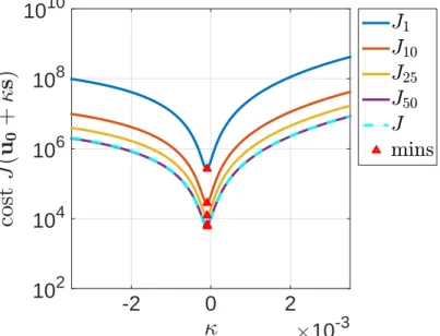
the optimal RMA cost as J?

n := Jn uMAPn

, and the optimal true cost as J? _:= _J _uMAP

. We wish to characterize the errors |J?

n−J?|and

uMAP_n −uMAP

for a given reduced misfit

dimension n. This is the subject of section 3.6.

3.6

Theoretical analysis of the randomized misfit approach

3.6.1 A guarantee of validity for the RMA solution with small n

For a given u in parameter space, it is clear that Jn(u;r) in (3.3) is an unbiased estimator of J(u). It is also clear from the Law of Large Numbers that Jn(u) converges

(39)

almost surely to its meanJ(u). However, demonstrating the efficacy of the randomized misfit

approachwith a small number of random realizations n, lies in exploiting a “concentration of measure” phenomenon in high dimensions. That is, the first step is to quantify convergence of Jn(u) close to its mean J(u).

This requires characterizing the exponential decay of the objective function error, which is parameterized by the reduced misfit dimension n.

We first show that errors larger thanδ/2, for a given δ >0, decay with a rate at least

as fast as the tail of a centered Gaussian. That is, for some distribution in (3.3) we have

P |Jn(u;r)−J(u)|> δ 2 ≤e−nI(δ), (3.5) where I(δ)≥c δ 2 2θ2. (3.6)

for some c >0 and some θ.

This rate is sufficient to guarantee the solution attained from the the randomized misfit approach is a discrepancy principle-satisfying solution for the original inverse prob-lem as will be shown in Theorem 2. Inequality (3.5) is equivalent to the statement that

P|Jn(u;r)−J(u)|> δ₂

satisfies a large deviation principle with large deviation rate func-tion I(δ) [139].

The following proposition may be viewed as a special case of Cramér’s Theorem, which states that a sample mean of i.i.d. random variables X asymptotically obeys a large deviation principle with rate I(δ) = sup_kkδ−ln_EekX [139]. However we require the exact non-asymptotic bounds as derived here to show convergence of the RMA forn=O(1). Recall that a real-valued random variableX isθ-subgaussianif there exists some θ >0such

that for all t ∈_R, _E

etX ≤eθ2t2/2.

Proposition 1. The RMA error|Jn(u;r)−J(u)|has a tail probability that decays exponen-tially innwith a nontrivial large deviation rate. Furthermore, if the RMA is constructed with

(40)

r such that 2|Jn(u;r)−J(u)| is the sample mean of i.i.d. θ-subgaussian random variables, then its large deviation rate is bounded below by c₂δ_θ22 for some c >0.

Proof. Givenr, define the random variable T(r;u) :=hr>db−Fb(u) i2 − bd−Fb(u) 2 . (3.7)

By a standard Chernoff bound (see, e.g.[71]), we have that the RMA tail error decays expo-nentially as P " 1 n n X j=1 T (rj;u)> δ # ≤e−nI(δ), (3.8) where I(δ) = maxt

tδ−ln_EetT(r;u) is the large deviation rate.

The second part of the proposition follows withc= 1 by bounding_EetT(r;u)in(3.8) and computing the maximum of tδ−θ2t2/2.

A large number of distributions are subgaussian, notably the Gaussian and Rademacher (also referred to as Bernoulli) distributions, and in fact any bounded random variable is sub-gaussian. One class of subgaussian distributions that provides additional computational efficiency is the following.

Definition 1 (`-percent sparse random variables [86, 96]). Let s = ₁₋1_` where ` ∈ [0,1) is the level of sparsity desired. Then

ζ = √s      +1 with probability ₂1_s, 0 with probability `= 1−1 s, −1 with probability ₂1_s (3.9) is a `-percent sparse distribution.

Note that for ` = 0, ζ corresponds to a Rademacher distribution, and that ` = 2/3

corresponds to the Achlioptas distribution [1]. By inspection we have that _E[ζ] = 0 and

(41)

The distributions arising from Definition 1 are well-suited for the randomized misfit approach. They are easy to implement, and the computation of the randomized misfit vector amounts to only summations and subtractions, adding a further speedup to the method. Increasing froms = 1tos >1results in a s-fold speedup as only1/sof the data is included. Note the RMA cost can be seen as the sum ofnrandom combinations from theN-dimensional misfit vector. Since each random combination has a different sparsity pattern, we effectively do not exclude any data, yet each computation requires only 1/s of the data.

The distributions defined by Definition 1, where 1 ≤ s < ∞, the random variable ζ distributed by Definition 1 haveEetζ≤e

b2t2

2 with b=

√

s−2 lns, ∀t∈(0,1]: Using the

inequality(2k)!≥2k_k_!and the Taylor expansion around ₀, for_t_∈₍₀_,_1]

Eetζ= 1 s ∞ X k=0 (st2)k (2k)! ≤ 1 s ∞ X k=0 (st2) 2k_k_! = 1 se s 2t 2 =e−lns+s2t 2 ≤e−t2lns+s2t 2 . (3.10)

So, the distributions defined Definition 1 are permitted in the following theorem, which defines the random projections that will lead to a RMA solution with a guarantee of validity.

Theorem 1. Definev:=d−b Fb(u)∈RN. Ifrin (3.7)has components that areb-subgaussian

for some b ≥ 1/√2, then the RMA error has a large deviation rate bounded below by c₂δ_θ22

for θ =kvk2/√2 and some 0< c < ₈1_b4.

Proof. Letr∈_RN _{such that}_r_{has i.i.d.} _b_{-subgaussian components} _r

i, withb ≥1/ √

2,

E[ri] = 0, and E[ri2] = 1. Define w= kvkv and X =r

>_w_{. Then} EetT=e−tkvk 2 E h etkvk2X2i ∀t∈_R. (3.11)

From [96, Lemma 2.2], E[X2] = 1 and X is also b-subgaussian. Then, by [64, Remark 5.1],

for 0≤t≤ 1 4b2,

E h

(42)

For0< t≤ 1 4b2_kvk2, we have E h etkvk2X2i≤1 +tkvk2 +tkvk4 E[X 4_] 2 + ∞ X k=3 1 4b2 k 4b2tkvk2k EX2k k! ≤1 +tkvk2 +t2kvk4E[X 4_] 2 + 4b 2_t_kvk23 ∞ X k=3 1 4b2 k EX2k k! ≤1 +tkvk2 +t2kvk4E[X 4_] 2 + 4b 2_t_kvk23 E h e41b2X2 i ≤1 +tkvk2 +t2kvk4E[X 4_] 2 + 64 √ 2b6t3kvk6 ≤1 +tkvk2 + 8b4t2kvk4+ 64√2b6t3kvk6 ≤etkvk2+8b4t2kvk4+64 √ 2b6_t3_kvk6 ,

using (3.12) in the fourth inequality and [134, p.93] in the fifth inequality. Let t? = ₈_b4_kvkδ 4_q

where q >1. Assuming kvk2 δ, we have that

Eet ?_T ≤e8b4t2?kvk4+64 √ 2b6_t3 ?kvk6 ₌_e δ2 8b4kvk4q2+ √ 2 δ3 8b6kvk6q3_. Then I(δ)≥δt?−lnE et?T_≥ 1− 1 q δ2 8b4_kvk4_q − √ 2 δ 3 8b6_kvk6_q3 ≥c δ kvk4, where 0< c < ₈1_b4. Taking 2θ2 =kvk

4 _{concludes the proof.}

A sharper result can be obtained for RMA constructed with b-subgaussian random variables where b ≤ 1. Note that this includes the distribution Definition 1 with s = 1

(Rademacher) and s= 3 (Achlioptas) by the above theorem. Following [64, (5)], let g be a standard Gaussian random variable, independent of all other random variables. Then, we have that for 0< t < _2kvk1 2,

E h etkvk2X i ≤_Eg " _N Y i eb2tkvk2w2ig2 # ≤_Eg h etkvk2g2 i = _q 1 1−2tkvk2 . (3.13)

(43)

So from (3.11) we have that EetT(u,r) ≤ e−tkvk2 q 1−2tkvk2 =e−tkvk2−12ln(1−2tkvk 2₎ . (3.14) Then tδ−ln (_E[T(u,r)])≥tδ+tkvk2+1 2ln 1−2tkvk 2 =:f(t). (3.15) Computing the derivative, we have that f(t) attains a maximum at

tmax = δ 2 kvk4+δkvk2. (3.16) Thus, we have maxf(t) = δ 2 2 kvk4+δkvk2 + δ 2 kvk2+δ + 1 2ln 1− δ kvk2 +δ = δ 2 2 kvk4+δkvk2 − 1 4 δ2 kvk2+δ2 − 1 6 δ3 kvk2 +δ3 − · · · = δ 2 4 kvk4+δkvk2 + 1 4 ( δ2 kvk4+δkvk2 − δ2 kvk2+δ2 ) − 1 6 δ3 kvk2+δ3 − · · · ≥c δ 2 kvk4,

where we employed the Taylor expansion in the second equality, and in the last inequalityc is some constant less than1/4. Note that the last inequality holds for δ kvk2 and taking

2θ2 ₌_kvk4 _{concludes the proof.}

The next theorem is the main research contribution of this chapter. It guarantees with high probability that the RMA solution will be a solution of the original problem under Morozov’s discrepancy principle, for relatively small n.

The theorem requires the following lemma, which defines the

Lemma 1. Let v :=db−Fb(u). Suppose that r is distributed such that the large deviation

rate of the RMA error is bounded below by c₂δ_θ22 for some c > 0 and θ =kvk

2

(44)

cost distortion tolerance ε >0 and a failure rate β >0, let n ≥ β

cε2. (3.17)

Then with probability at least 1−e−β_,

(1−ε)kvk2 ≤ 1 n n X j=1 r>_j v2 ≤(1 +ε)kvk2, (3.18) and hence, (1−ε)J(u)≤Jn(u;r)≤(1 +ε)J(u). (3.19)

Proof. The proof follows from setting δ =εkvk2 in (3.5).

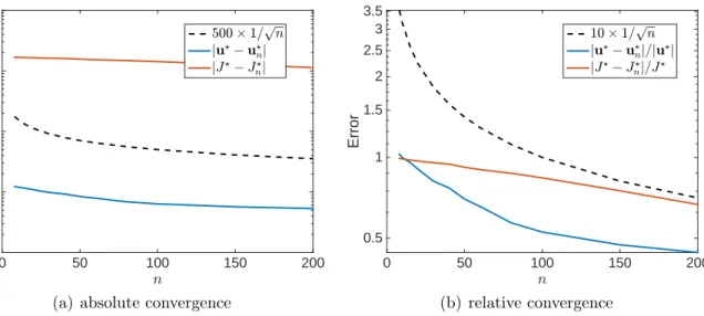
This lemma demonstrates a remarkable fact that with n i.i.d. draws one can reduce the data misfit dimension fromN ton while bearing a relative error ofε=O(1/√n) in the

cost function, where the reduced dimensionn is independent of the dimensionN of the data. This idea is the basis for data-reduction techniques via variants of the Johnson-Lindenstrauss Lemma in existing work with random projections (see e.g. [48,60,91]). With the connection through the randomized misfit approach, the ubiquitous N-independent Monte Carlo factor ε=O(1/√n) in Johnson-Lindenstrauss literature can thus be understood by reframing the

application of a random projection as a Monte Carlo method in the form of (3.18).

Unlike other applications of the Monte Carlo method, e.g. Markov chain Monte Carlo, in whichn must be large to be successful,n can be moderate or small for inverse problems, depending on the noise η in (2.2). In the following theorem we show this is possible via

Morozov’s discrepancy principle [101]. To avoid over-fitting the noise, from (2.1) one seeks a MAP point uMAP such that

d_j −w x_j;uMAP ≈σ, i.e. db−F ub MAP 2 ≈N. We say that an inverse solution uMAP _{satisfies Morozov’s discrepancy principle with parameter} _τ _if

bd−F ub MAP 2 =τ N (3.20) for some τ ≈1.

(45)

Theorem 2 (Statistical Morozov’s discrepancy principle). Suppose that the conditions of Lemma 1 are met. If uMAP_n is a discrepancy principle-satisfying solution for the RMA cost, i.e., Jn uMAPn ,r := 1 n n X j=1 h r>_j db−F ub MAP_n i2 =τ0N (3.21) for someτ0 ≈1, then with probability at least 1−e−β, uMAP_n is also a solution for the original problem that satisfies Morozov’s discrepancy principle with parameter τ, i.e.

J uMAP_n := db−F ub MAP n 2 =τ N. (3.22) for τ ∈ _τ0 1+ε, τ0 1−ε .

Proof. The claim is a direct consequence of (3.18). 3.6.2 Other theoretical results

We are now in the position to show a different proof of the Johnson-Lindenstrauss embedding theorem using a stochastic programming derivation of the RMA. Following [129], we define a mapS from_Rn _to

RN, where nN, to be a Johnson-Lindenstrauss transform

(JLT) if

(1−ε)kvk2 ≤ kSvk2 ≤(1 +ε)kvk2, (3.23) holds with some probability p=p(n, ε), where ε >0.

Theorem 3 (Johnson-Lindenstrauss embedding theorem [42, 64, 96]). Suppose that r is distributed such that the large deviation rate of the RMA error is bounded below by c₂δ_θ22 for

some c >0 and some θ. Let 0< ε < 1, vi ∈ RN, i= 1, . . . , m, and n =O(ε−2lnm). Then

there exists a map F :_RN →_Rn _{such that}

(46)

Proof. The conditions of Lemma 1 hold, thus for a givenv∈_RN_{, note that} _(3.18)_is equivalent to (1−ε)kvk2 ≤ kΣvk2 ≤(1 +ε)kvk2, (3.25) where Σ:= √1 n [r1, . . . ,rn] > . (3.26)

DefineF(v) := Σv. Inequality(3.24)is then a direct consequence of(3.25)for a pair(vi,vj) with probability at least 1−e−c2nε2. Using an union bound over all pairs, claim (3.24)holds

for any pair with probability at least 1−m−α _if _n _≥_c(2+α)

ε2 lnm.

As discussed above,Jn(u;r)is an unbiased estimator ofJ(u). It is therefore reason-able to expect that J_n? := minuJn(u;r)converges to J? := minuJ(u). The following result

[132, Propositions 5.2 and 5.6] states that under mild conditions J?

n in fact converges to J?. It is not unbiased, but is however downward biased.

Proposition 2. Assume that Jn(u;r) converges to J(u) with probability 1 uniformly in u, then J_n? converges to J? with probability 1. Furthermore, it holds that

E[Jn?]≤E J_n?₊₁ ≤J?, (3.27) that is, J? n is a downward-biased estimator of J?.

Stochastic programming theory gives a stronger characterization of this convergence. One can show thatuMAP

n converges weakly touMAP with ann

−1

2 rate. IfJ(u)is convex with

finite value, thenuMAP

n =uMAP with probability exponentially converging to1. See Chapter 5 in [132] for details. For a linear forward map F(u) =Fu, that is, J(u) is quadratic, we

can derive a bound on the solution error using the spectral norm of F.

Theorem 4. Suppose the conditions of Lemma 1 hold. Let m := rank(Fb). Then

(47)

ii) if F is linear, then with probability at least 1−m−α uMAP_n −uMAP ≤ ε σ2 min(G) Fb uMAP + bd Fb , (3.28) where G:=Fb>ΣΣ>Fb+C−1 1₂ , and n=O(ε−2(2 +α) lnm).

Proof. The first assertion follows from(3.19)and the definition ofuMAP

n (3.4), indeed J_n? =Jn uMAPn

≤J uMAP≤(1 +ε)J uMAP = (1 +ε)J?, (3.29)

and the other direction is similar. For the second assertion, note that uMAP and uMAP_n are solutions of the following first optimality conditions

b F>Fb+C−1 u? =Fb>db+C−1u₀, (3.30a) b F>ΣΣ>Fb +C −1 uMAP_n =Fb > ΣΣ>db+C−1u₀. (3.30b)

Defines∆ :=uMAP−uMAP_n . An algebraic manipulation of (3.30) gives

b F>ΣΣ>Fb+C−1 s∆ = b F>ΣΣ>Fb −Fb>Fb uMAP+Fb>db−Fb>ΣΣ>d.b (3.31)

Taking the inner product of both sides with s∆we have

D s∆,FbTΣΣTFb+C−1 s∆E=DFsb ∆,ΣΣTFub ? −Fub ? E + D b Fs∆,db−ΣΣTdb E . (3.32) Then we can bound the left-hand side of (3.32):

D s∆, b F>ΣΣ>Fb+C−1 s∆ E ≥σ2_min(G)s∆2. (3.33) To bound terms on right hand side of (3.32), we need the following straightforward variant of (3.25), i.e. ∀v∈_RN _and _n₌_O₍_ε−2₎_:

ΣΣ

>

(48)

Using the Cauchy-Schwarz inequality we have D b Fs∆,ΣΣTFub ?−Fub ? E ≤ε Fb 2 ks∆k ku?k, (3.35a) D b Fs∆,db−ΣΣTdb E ≤ε Fb ks∆k db , (3.35b)

where we have used(3.34)and definition of matrix norm. Next, combining (3.35)and(3.33)

ends the proof.

Note that for inequalities in (3.35) to be valid, it is sufficient to choose n, α, ε such that (3.34) is valid for m basis vectors spanning the column space of Fb, and hence n =

O(ε−2(2 +α)