A Universal Pricing Framework for Guaranteed Minimum Benefits in Variable Annuities *

Guaranteed Minimum Benefits in Variable Annuities

* Daniel Bauer

Research Training Group 1100, Ulm University Helmholtzstraße 18, 89069 Ulm, Germany Phone: +49 (731) 5031088, Fax: +49 (731) 5031239

[email protected] Alexander Kling†

Institut für Finanz- und Aktuarwissenschaften Helmholtzstraße 22, 89081 Ulm, Germany Phone: +49 (731) 5031242, Fax: +49 (731) 5031239

[email protected] Jochen Russ

Institut für Finanz- und Aktuarwissenschaften Helmholtzstraße 22, 89081 Ulm, Germany Phone: +49 (731) 5031233, Fax: +49 (731) 5031239

[email protected]

Abstract

Variable Annuities with embedded guarantees are very popular in the US-market. There exists a great variety of products with both, guaranteed minimum death benefits (GMDB) and guaranteed minimum living benefits (GMLB). Although several approaches for pricing some of the corresponding guarantees have been proposed in the academic literature, there is no general framework in which the existing variety of such guarantees can be priced consistently. The present paper fills this gap by introducing a model, which permits a consistent and extensive analysis of all types of guarantees currently offered within Variable Annuity contracts. Besides a valuation assuming that the policyholder follows a given strategy with respect to surrender and withdrawals, we are able to price the contract under optimal policyholder behavior. Using both, Monte-Carlo methods and a generalization of a finite mesh discretization approach proposed by Tanskanen and Lukkarinen (2004), we find that some guarantees are overpriced, whereas others, e.g. guaranteed annuities within guaranteed minimum income benefits (GMIB), are offered significantly below their risk-neutral value.

Keywords: Risk-Neutral Valuation, Guaranteed Minimum Benefits, Embedded Options, Variable Annuity, Monte-Carlo-Simulation, Discretization Methods

1

Introduction

Variable Annuities, i.e. deferred annuities that are fund-linked during the deferment period were introduced in the 1970s in the United States (see Sloane (1970)). Starting in the 1990s, insurers included certain guarantees in such policies, namely guaranteed minimum death benefits (GMDB) as well as guaranteed minimum living benefits (GMLB). The GMLB options can be categorized in three main groups: Guaranteed minimum accumulation benefits (GMAB) provide a guaranteed minimum survival benefit at some specified point in the future to protect policyholders against decreasing stock markets. Products with guaranteed minimum income benefits (GMIB) come with a similar guaranteed value G at some point in time T. However, the guarantee only applies if this guaranteed value is converted into an annuity using given annuitization rates. Thus, besides the standard possibilities to take the market value of the fund units (without guarantee) or convert the market value of the fund units into a lifelong annuity using the current annuity conversion rates at time T, the GMIB option gives the policyholder a third choice, namely converting some guaranteed amount G

into an annuity using annuitization rates that are fixed at inception of the contract (t=0). The third kind of guaranteed minimum living benefits are so-called guaranteed minimum withdrawal benefits (GMWB). Here, a specified amount is guaranteed for withdrawals during the life of the contract as long as both the amount that is withdrawn within each policy year and the total amount that is withdrawn over the term of the policy stay within certain limits. Commonly, guaranteed annual withdrawals of up to 7% of the (single up-front) premium are guaranteed under the condition that the sum of the withdrawals does not exceed the single premium. Thus, it may happen that the insured can withdraw money from the policy, even if the value of the account is zero. Such guarantees are rather complex since the insured has a broad variety of choices.

Most of the earlier literature on Variable Annuities, e.g., Rentz Jr. (1972) or Greene (1973) is empirical work dealing with product comparisons rather than pricing issues. It was not until recently, that the special types of guarantees were discussed by practitioners (cf. JPMorgan (2004), Lehman Brothers (2005)), or analyzed in the academic literature.

Milevsky und Posner (2001) price various types of guaranteed minimum death benefits. They present closed form solutions for this “Titanic Option”3 _{in case of an exponential mortality} law and numerical results for the more realistic Gompertz-Makeham law. They find that in general these guarantees are overpriced in the market.

In Milevsky und Salisbury (2002), a model for the valuation of certain GMLB and GMDB options is presented in a framework where the insured has the possibility to partially surrender the policy. The authors call this a “Real Option to Lapse”4_{. They present closed}

3 _{The authors denote this option as “Titanic Option” since the payment structure falls between}

European and American Options and the payment is triggered by the decease of the insured.

form solutions in the case of an exponential mortality law, constant surrender fees and no maturity benefits. It is shown that both, the value and the optimal surrender strategy, are highly dependent on the amount of the guarantee and of the surrender fee.

In Milevsky und Salisbury (2006), the same authors price GMWB options. Besides a static approach, where deterministic withdrawal strategies are assumed, they calculate the value of the option in a dynamic approach. Here, the option is valuated under optimal policyholder behavior. They show that under realistic parameter assumptions optimally at least the annually guaranteed withdrawal amount should be withdrawn. Furthermore, they find that such options are usually underpriced in the market.

In spite of these approaches for the pricing of several options offered in Variable Annuities, there is no general framework in which the existing variety of such options can be priced consistently and simultaneously. The present paper fills this gap. In particular, we present a general framework in which any design of options and guarantees currently offered within Variable Annuities can be modeled. Besides the valuation of a contract assuming that the policyholder follows a given strategy with respect to surrender and withdrawals, we are able to determine an optimal withdrawal and surrender strategy, and price contracts under this

rational strategy.

The rest of the paper is organized as follows. In Section 2, we give a brief overview over the existing forms of guarantees in Variable Annuities. Section 3 introduces the general pricing framework for such guarantees. We show how any particular contract can be modeled within this framework. Furthermore, we explain how a given contract can be priced assuming both, deterministic withdrawal strategies and “optimal” strategies. The latter is referred to as the case of rational policyholders. Due to the complexity of the products, in general there are no closed form solutions for the valuation problem. Therefore, we have to rely on numerical methods. In Section 4, we present a Monte Carlo algorithm as well as a discretization approach based on generalizations of the ideas of Tanskanen und Lukkarinen (2004). The latter enables us to price the contracts under the assumption of rational policyholders. Our results are presented in Section 5. We present the values for a variety of contracts, analyze the influence of several parameters and give economic interpretations. Section 6 closes with a summary of the main results and an outlook for future research.

2

Guaranteed Minimum Benefits

This Section introduces and categorizes predominant guarantees offered within Variable Annuity contracts. After a brief introduction of Variable Annuities in general in Section 2.1, we dwell on the offered Guaranteed Minimum Death Benefits (Section 2.2) and Guaranteed Minimum Living Benefits (Section 2.3). We explain the guarantees from the customer’s point of view and give an overview over fees that are usually charged.

2.1

Variable Annuities

Variable Annuities are deferred, fund-linked annuity contracts, usually with a single premium payment up-front. Therefore, in what follows we restrict ourselves to single premium policies. When concluding the contract, the insured are frequently offered optional guarantees, which are paid for by additional fees.

The single premium P is invested in one or several mutual funds. We call the value Atof the

insured’s individual portfolio the insured’s account value. Customers can usually influence the risk-return profile of their investment by choosing from a selection of different mutual funds. All fees are taken out of the account by cancellation of fund units. Furthermore, the insured has the possibility to surrender the contract, to withdraw a portion of the account value (partial surrender), or to annuitize the account value after a minimum term.

The following technical terms are needed to describe the considered guarantees: The ratchet benefit base at a certain point in time t is the maximum of the insured’s account value at certain previous points in time. Usually, it denotes the maximum value of the account on all past policy anniversary dates. This special case is also referred to as annual ratchet benefit base. In order to simplify notation, in what follows, we only consider products with annual ratchet guarantees.

Furthermore, the roll-up benefit base is the theoretical value that results from compounding the single premium P with a constant interest rate of i % p.a. We call this interest rate the

roll-up rate.

2.2

Guaranteed Minimum Death Benefits

If the insured dies during the deferment period, the dependants obtain a death benefit. When Variable Annuities were introduced, a very simple form of death benefit was predominant in the market. However, since the mid 1990s, insurers started to offer a broad variety of death benefit designs (cf. Lehmann Brothers (2005)).

The basic form of a death benefit is the so-called Return of Premium Death Benefit. Here, the maximum of the current account value at time of death and the single premium is paid. The price for this kind of benefit usually is already included in the charges of the contract, i.e. this option is available without additional charges.

Another variant is the Annual Roll-Up Death Benefit. Here, the death benefit is the maximum of the roll-up benefit base (often with a roll-up rate of 5% or 6%) and the account value. A typical fee for that death benefit with a roll-up rate of 6% is approximately 0.25% p.a. of the account value (see, e.g., JPMorgan (2004)).

If the contract contains an Annual Ratchet Death Benefit, the death benefit consists of the greater of the annual ratchet benefit base and the current account value. The charges for this type of death benefit are similar.

Furthermore, the variant Greater of Annual Ratchet or Annual Roll-Up Death Benefit is offered. With this kind of option, the greater of the roll-up benefit base and the annual ratchet benefit base, but at least the current account value is paid out as the death benefit. With a roll-up rate of i=6%, insurers typically charge about 0.6% p.a. for this guarantee (see, e.g., JPMorgan (2004)).

2.3

Guaranteed Minimum Living Benefits

It was not until the late 1990s that Guaranteed Minimum Living Benefits have been offered in the market. Today, GMLB are very popular.

The two earliest forms, Guaranteed Minimum Accumulation Benefits (GMAB) and Guaranteed Minimum Income Benefits (GMIB) originated almost at the same time. Both guarantees offer the insured a guaranteed maturity benefit, i.e. a minimum benefit at the maturity T of the contract. However, with the GMIB, this guarantee only applies if the account value is annuitized. Since 2002, a new form of GMLB is offered, the so-called Guaranteed Minimum Withdrawal Benefit (GMWB). Here, the insured is entitled to withdraw a pre-specified amount annually, even if the account value has fallen below this amount. These guarantees are extremely popular. In 2004, 69% of all Variable Annuity contracts sold included a GMWB option. Each of the 15 largest Variable Annuity providers offered this kind of guarantee at this time (cf. Lehmann Brothers (2005)).

2.3.1 Guaranteed Minimum Accumulation Benefits (GMAB)

Guaranteed Minimum Accumulation Benefits are the simplest form of guaranteed living benefits. Here, the customer is entitled to a minimal account value at maturity T of the contract. Usually, is the single premium P, sometimes a roll-up benefit base. The corresponding fees vary between 0.25% and 0.75% p.a. of the account value (cf. Mueller (2006)). A T G A T G

2.3.2 Guaranteed Minimum Income Benefits (GMIB)

At maturity of a Variable Annuity with a GMIB, the policyholder can as usual choose to obtain the account value (without guarantee) or annuitize the account value at current market conditions (also without any guarantee). However, the GMIB option offers an additional choice: The policyholder may annuitize some guaranteed amount at annuitization rates that have been specified up-front. Therefore, this option can also be interpreted as a guaranteed annuity, starting at t=T, where the annuity payments have already been specified at t=0.

I T

G

Note that if the account value at maturity is below the guaranteed value , the customer cannot take out the guaranteed capital as a lump sum but only in the form of an annuity at the pre-specified annuitization rates. Thus, the option is “in the money” at time T if the

I T G I T G

resulting annuity payments exceed the annuity payments resulting from converting the actual account value at current annuity rates.

The guaranteed amount I usually is a roll-up benefit base with, e.g., i

T

G = 5% or 6%, or a

ratchet benefit base. Sometimes there is not one specified maturity, but the policyholder can annuitize within a certain (often rather long) time period. The offered roll-up rates frequently exceed the risk-free rate of interest, whereas the pre-specified annuitization factors are usually rather conservative. Thus, at maturity the option might not be in the money, even if the guaranteed amount exceeds the account value. Furthermore, the pricing of these guarantees is often based on certain assumptions about the customers’ behavior rather than assuming that everybody exercises the option when it is in the money. Such assumptions of course reduce the option value.5 _{Depending on the specific form of the guarantee, the} current fees for GMIB contracts typically vary between 0.5% and 0.75% p.a. of the account value.

2.3.3 Guaranteed Minimum Withdrawal Benefits (GMWB)

Products with a GMWB option give the policyholder the possibility to withdraw a specified amount (usually the single premium) in small portions. Typically, the insured is entitled to annually withdraw a certain proportion x

W

G₀

W of this amount , even if the account value

has fallen to zero. At maturity, the policyholder can take out or annuitize any remaining funds if the account value did not vanish due to such withdrawals.

W

G₀

Recently, several forms of so-called Step-up GMWB options have been introduced: With one popular version, the total guaranteed amount which can be withdrawn is increased by a predefined ratio at certain points in time, if no withdrawals have been made so far. In what follows, we will only analyze this form of Step-up GMWB. Alternatively, there are products in the market, where at certain points in time, the remaining total guaranteed amount which can be withdrawn is increased to the maximum of the old remaining guaranteed amount and the current account value.

The latest development in this area are so-called “GMWB for life” options, where only some maximum amount to be withdrawn each year is specified but no total withdrawal amount. This feature can be analyzed within our model by letting _GW =∞ and

0 T =∞.

From a financial point of view, GMWB options are highly complex, since the insured can decide at any point in time whether and, if so, how much to withdraw. They are currently offered for between 0.4% and 0.65% p.a. of the account value. However, Milevsky and Salisbury (2006) find that these guarantees are substantially underpriced. They conclude

that insurers either assume a suboptimal customer behavior or use charges from other (overpriced) guarantees to cross-subsidize these guarantees.

While this summary of GMDB and GMLB options covers all the basic designs, a complete description of all possible variants would be beyond the scope of this paper. Thus, some products offered in the market may have features that differ from the descriptions above.6 Our model and notation presented in the following Section is designed to cover all the guarantees described in this Section as special cases. Of course, the underlying general framework allows for any specific variations of the guarantees that might deviate from the products described above.

3

A General Valuation Framework for Guaranteed Minimum

Benefits

3.1

The Financial Market

T t t ∈0,

As usual in this context, we assume that there exists a probability space (Ω,F,Q) equipped with a filtration F=

( )

ℑ _{[ ]}

T t t

B _∈0,

, where Q is a risk-neutral measure under which payment streams can be valued as expected discounted values.7 _{Existence of this measure also} implies that the financial market is arbitrage free. We use a bank account _] as the numéraire process, which evolves according to

( )

_[ 0 , ₀ > =r dt B B dB t t t _{. (1)}

Here, rtdenotes the short rate of interest at time t.

We further assume that the underlying mutual fund St of the Variable Annuity is modeled as

a right-continuous F –adapted stochastic process with finite left hand limits (RCLL).8 _In particular, the discounted asset process

[ ]T t t t B S , 0 ∈ ⎟⎟ ⎠ ⎞ ⎜⎜ ⎝ ⎛

is a Q-martingale. For convenience, we assume S₀ =B₀ =1.

6 _{For current information regarding Variable Annuity products, types of guarantees, and current fees,}

we refer, e.g., to www.annuityfyi.com.

7 _{This is a consequence of the risk-neutral valuation formula, cf. Bingham and Kiesel (2004).}

8 _{For our numerical calculations, we assume that S evolves according to a geometric Brownian motion}

3.2

A Model for the Insurance Contract

Within the following model, any kind of Variable Annuity contract which contains one or more of the guarantees introduced in Section 2 can be represented. In our numerical analysis, we restrict ourselves to contracts with at most one GMDB and one GMLB option. We consider a Variable Annuity contract with a finite integer maturity T, which is taken out at time for a single premium P. Although the model generally allows for flexible expiration options, in order to simplify the notation, we only consider a fixed maturity T. We denote the account value by A

0

= t

t and ignore any up-front charges. Therefore, we haveA₀ =P .

During the term of the contract, we only consider the charges which are relevant for the guarantees, i.e. continuously deducted charges for the guarantees and a surrender fee. The surrender fee is charged for any withdrawal of funds from the contract except for guaranteed withdrawals within a GMWB option. The continuously deducted guarantee fee

ϕ is proportional to the account value and the surrender fee s is proportional to the respective amount withdrawn.

In order to valuate the benefits of the contract, we start by defining two virtual accounts: Wt

denotes the value of the cumulative withdrawals up to time t. We will refer to it as the

withdrawal account. Every withdrawal is credited to this account and compounded with the risk-free rate of interest up to maturity T. At time zero, we have W0 = 0.

Similarly, by Dt we denote the value of the death benefits paid up to time t. Analogously to

the withdrawals, we credit death benefit payments to this death benefit account and compound the value of this account with the risk-free rate until time T. Since we assume the insured to be alive at time zero, we obviously have D0 = 0.

In order to describe the evolution of the contract and the embedded guarantees, we also need the following processes:

The guaranteed minimum death benefit at time t is denoted by . Thus, the death benefit at time t is given by D t G

{

D

}

t t G A ;

max . We let if the contract contains one of the described GMDB options (cf. Section

0 0 A

GD ₌

2.2), otherwise we let . The evolution of over time depends on the type of the GMDB option included in the contract. It will be described in detail in Section

0 0D = G D t G 3.3.

The guaranteed maturity benefit of the GMAB option is denoted by . In order to account for possible changes of the guarantee over the term of the contract, we let

A T

G

( )

GtA t∈_{[ ]}0,T

represent the evolution of this guarantee (see Section 2.3.1 for details). We have

for contracts with one of the described GMAB options and for contracts without a GMAB option. 0 0 A G A ₌ 0 0A = G

Analogously, we let denote the guaranteed maturity benefit that can be annuitized in the case of a GMIB option and model its development by

I T G

( )

t [ ]T I t G _∈0, . Also, we have and for contracts with and without a GMIB option, respectively.

0 0 A GI _{= 0} 0 = I G

Finally, to be able to represent GMWB options, we introduce the processes

( )

G_tW _{t∈[ ]0,T} and

( )

[ ]. denotes the remaining total amount that can be withdrawn after time t, and is the maximum amount that can be withdrawn annually due to the GMWB option. If the contract contains a GMWB, we let and , where is the portion of the premium that can be withdrawn annually. For contracts without GMWB, we let . The evolution over time of these processes is also explained in detail in Section T t E t G _∈0, W t G E t G 0 0 A GW ₌ 0 0 x A GE = W xW 0 0 0W =GE = G 3.3.

Due to the Markov-property9 _{of the underlying processes, all information available at time t} is completely contained in the so-called state variables At , Wt, , , , , and . To simplify notation, we introduce the following state vector

t D A t G I t G D t G W t G E t G

(

E

)

t W t D t I t A t t t t t A W D G G G G G y = , , , , , , , .

3.3

Evolution of the Insurance Contract

During the term of the contract there are four possible types of events: the insured can

• withdraw funds as a guaranteed withdrawal of a GMWB option,

• perform a partial surrender, i.e. withdraw more than the guaranteed withdrawal amount,

• completely surrender the contract, or

• pass away.

For the sake of simplicity, we assume that all these events can only occur at a policy anniversary date. Therefore, at integer time points t =1,2,...,T , for all state variables we distinguish between and , i.e. the value immediately before and after the occurrence of such events, respectively.

− ⋅)t ( _⋅ + t ) (

The starting values at of all accounts and processes describing the contract were given in Section

0

= t

3.2. Now, we will describe their evolution in two steps: First, for t =0,1,2,...,T −1, the development within a policy year, i.e. from t+ _{to (t+1)}- _{is specified. Subsequently, we will}

describe the transition from (t+1)- _{to (t+1)}+_{, which depends on the type of guarantees}

included in the contract and the occurrence of the described events. Finally, we describe the maturity benefits of the contract.

3.3.1 Development between t+ and (t+1)-

As indicated in Section 3.1, the price of the underlying mutual fund evolves stochastically over time. Thus, taking into account continuous guarantee fees ϕ, for the account value we have − + + −ϕ + = _S ⋅e S A A t t t t 1 1 . (2)

The accounts Wt and Dt are compounded with the risk-free rate of interest, i.e.

∫ = + + − + 1 1 t t sds r t t W e W and − + ∫ . + + = 1 1 t trsds t t D e D

The development of the processes , and depends on the specification of the corresponding GMDB, GMAB and GMIB option: if the corresponding guaranteed benefit is the single premium or if the option is not included, we let . If the guaranteed benefit is a roll-up base with roll-up rate i, we set . For ratchet guarantees, we have , since the ratchet base is adjusted after possible withdrawals, and therefore considered in the transition from (t+1)

D t G A t G I T G + − + A I = tD A I D t G G / / / / 1

(

i G G D A I t I A D t+1/ / − = / / + 1+

)

+ − + A I = tD A I D t G G / / / / 1 - _{to (t+1)}+ _{(cf. Section} 3.3.2).

The processes W and do not change during the year, i.e. .

t G E t G − + + E = tW E W t G G / / 1 3.3.2 Transition from (t+1)- _{to (t+1)}+

At the policy anniversary date, we distinguish four cases: a) The insured dies within the period (t,t+1]

Since our model only allows for death at the end of the year, dying within the period (t,t+1] is equivalent to a death at time t+1. The death benefit is credited to the death benefit account and will then be compounded with the risk-free rate until maturity T:

. Since after death, no future benefits are possible, we let as well as . The withdrawal account, where possible prior withdrawals have been collected, will not be changed, i.e.

} ; max{ _{1 1} 1 1 −+ +− −+ + + = t + tD t t D G A D 0 1 = + + t A / / / / 0 1 + = +I W D E A t G − + + +1 = t 1 t W

W . This account will be compounded until maturity.

b) The insured survives the year (t,t+1] and does not take any action (withdrawal, surrender) at time t+1

Here, neither the account D nor W is changed. Thus, we have − , and

+ + +1 = t 1 t A A − + + +1 = t 1 t D D − + + +1 = t 1 t W

W . For the GMAB, GMIB, and GMDB, without a ratchet type guarantee, we also have . If, however, one or more of these guarantees are of ratchet type, we adjust the corresponding guarantee account by

− + + + I D = tA I D A t G G / / 1 / / 1

{

+

}

+ − + + +/1I/D =max tA/1I/D ; t 1 A t G A G .

If the contract includes a GMWB option with step-up and t+1 is a step-up point, the GMWB processes are adjusted according to the step-up feature, but only if there were no past withdrawals: If denotes the factor, by which the total amount to be withdrawn is increased (cf. Section 2.3.3), we get

1 + t W i { }

(

1 0 1

)

1 1 = 1+Ι −+ = ⋅ + − + + + Wt Wt W t W t G i G and . In

any other case, we have .

+ + + + = W ⋅ tW E t x G G _{1 1} − + + + E = tW E W t G G / 1 / 1

c) The insured survives the year (t,t+1] and withdraws an amount within the limits of the GMWB option

A withdrawal within the limits of the GMWB is a withdrawal of an amount

{

−

}

+ − + + ≤ tE tW t G G

E ₁ min ₁; ₁ , since the withdrawn amount may neither exceed the maximal annual withdrawal amount − nor the remaining total withdrawal amount .

+ E t G ₁ − + W t G ₁

The account value is reduced by the withdrawn amount. In case the withdrawn amount exceeds the account value, the account value is reduced to 0. Thus, we have

{

1 1

}

1 max 0; −+ +

+

+ = t − t

t A E

A . Also, the remaining total withdrawal amount is reduced by the withdrawn amount, i.e. . Furthermore, the withdrawn amount is credited to the withdrawal account:

1 1 1 + − + + + = tW − t W t G E G 1 1 1 −+ + + + = t + t t W E

W . The maximal annual withdrawal amount as well as the death benefit account remain unchanged: − and .

+ + + = tE E t G G _{1 1} − + + +1 = t 1 t D D

Usually, living benefit guarantees (GMAB and GMIB) and, in order to avoid adverse selection effects, also the guaranteed death benefits are reduced in case of a withdrawal. We will restrict our considerations to a so-called pro rata adjustment. Here, guarantees which are not of ratchet type are reduced at the same rate as the account value, i.e.

− + − + + + + + ⎟⎟ ⎠ ⎞ ⎜⎜ ⎝ ⎛ = A I D t t t D I A t _A G A G / / 1 1 1 / /

1 . If one or more of the guarantees are of ratchet type, for the respective guarantees, we let

⎪⎭ ⎪ ⎬ ⎫ ⎪⎩ ⎪ ⎨ ⎧ ⎟⎟ ⎠ ⎞ ⎜⎜ ⎝ ⎛ = − + − + + + + + + + D I A t t t t D I A t _A G A A G / / 1 1 1 1 / / 1 max ; .10

d) The insured survives the year (t,t+1] and withdraws an amount exceeding the limits of the GMWB option

At first, note that this case includes the following cases as special cases:

d1) The contract does not comprise a GMWB option and an amount is withdrawn. − + + < < 1 1 0 E_t A_t

d2) A GMWB option is included in the contract, but the insured withdraws an amount with − + + < < 1 1 0 E_t A_t

{

−

}

+ − + + > tE tW t G G E ₁ min ₁; ₁ .

d3) The insured surrenders by withdrawing the amount − 11

+ +1 = t 1 t A E . We let 2 , where 1 1 1 1 + + + = t + t t E E E

{

−

}

+ − + + = tE tW t G G E1 _{1 1}

1 min ; . Consequently, is the portion of the withdrawal within the limits of the GMWB option. If the contract does not include a GMWB option, we obviously have .

1 1 + t E 0 1 1 = + t E

As in case c), the account value is reduced by the amount withdrawn, i.e. , and the withdrawn amount is credited to the withdrawal account. However, the insured has to pay a surrender fee for the second component which leads to

1 1 1 + − + + + = t − t t A E A

(

s E E W

)

W_t++ = _t−+ + _t+ + _t2+1 ⋅ 1− 1 1 1

1 . The death benefit account remains unchanged, i.e. . − + + +1 = t 1 t D D

10 _{Besides pro rata adjustments, there are also reductions by the so-called dollar method. Here, all the respective} processes are reduced by the withdrawn amount, i.e. max

[

/ / ₁,0

]

1 / / 1 + + − + +I D = tA I D − t A t G E

G . In order to model and evaluate products where the dollar method or any other reduction scheme applies, the respective formulas can be adjusted.

11 _{If the contract comprises a GMWB option and if}

{

−

}

+ − + − + ≤ tE tW t G G

A 1 min 1; 1 as well as , then a withdrawal of is within the limits of the GMWB and does not lead to a surrender of the contract. However, this case is covered by case c).

− + − + < tW t G A 1 1 − + +1 = t 1 t A E

Again, the future guarantees are modified by the withdrawal: For the guarantees which are

not of ratchet type, we have −

+ − + + + + + ⎟⎟ ⎠ ⎞ ⎜⎜ ⎝ ⎛ = A I D t t t D I A t _A G A G / / 1 1 1 / /

1 , whereas for the ratchet type guarantees, we let ⎪⎭ ⎪ ⎬ ⎫ ⎪⎩ ⎪ ⎨ ⎧ ⎟⎟ ⎠ ⎞ ⎜⎜ ⎝ ⎛ = − + − + + + + + + + D I A t t t t D I A t _A G A A G / / 1 1 1 1 / / 1 max ; .

For contracts with a GMWB, withdrawing an amount

{

−

}

+ − +

+ > tE tW

t G G

E ₁ min ₁; ₁ also changes future guaranteed withdrawals. We consider a common kind of GMWB12 _{option, where the} guaranteed future withdrawals are reduced according to

⎭ ⎬ ⎫ ⎩ ⎨ ⎧ ⋅ − = ₋ + + + − + + − + + + 1 1 1 1 1 1 min ; t t W t t W t W t _A A G E G G ,

i.e. the withdrawal amount is reduced by the higher of a pro rata reduction and a reduction according to the dollar method. For future annual guaranteed amounts, we use

− + + + − + + + = ⋅ 1 1 1 1 t t E t E t _A A G G .13 3.3.3 Maturity Benefits at T

If the contract neither comprises a GMIB nor a GMAB option, the maturity benefit LT is

simply the account value, i.e. . In contracts with a GMAB option, the survival benefit at maturity is at least the GMAB, thus

+ = _T T A L

{

+ +

}

= A T T A T A G L max ; .

Insured holding a GMIB option can decide whether they want a lump sum payment of the account value or annuitize this amount at current annuitization rates. Alternatively, they can annuitize the guaranteed annuitization amount at pre-specified conditions. If we denote by and the annuity factors

+

T

A

current

ä äguar 14 when annuitizing at the current and the

guaranteed, pre-specified conditions, respectively, the value of the guaranteed benefit at maturity is given by guar current I T _ä ä

G + ⋅ _{. Thus, a financially rational acting customer will chose the}

annuity, whenever we have + _{⋅ >} +

T A ä ä G guar current I

T . Therefore, the value of the benefit at time T is given by ⎪⎭ ⎪ ⎬ ⎫ ⎪⎩ ⎪ ⎨ ⎧ ⋅ = + + guar current I T T I T _ä ä G A L max ; . 12 _{Cf. Pioneer (2005), pp. 36.}

13 _{Cf. Pioneer (2005), page 36f. Also, a reduction of the form}

− + + + − + + + = ⋅ W t W t E t E t G _GG G 1 1 1 1 is frequently offered. 14 _{Here, an annuity factor is the price of an annuity paying one dollar each year.}

If the contract contains both, a GMAB and a GMIB option, the maturity value of the contract is

{

I

}

T A T T L L L =max ; .

3.4

Contract Valuation

We make the common assumption that financial markets and biometric events are independent. Furthermore, we assume risk-neutrality of the insurer with respect to biometric risks (cf. Aase and Persson (1994)). Thus, the risk-neutral measure for the combined market (insurance and financial market) is the product measure of Q and the usual measure for biometric risks. In order to keep the notation simple, in what follows, we will also denote this product measure by Q. Even if risk-neutrality of the insurer with respect to biometric risk is not assumed, there are still reasons to employ this measure for valuation purposes (see Møller (2001)).

Let be the insured’s age at the start of the contract and denote the probability for a -year old to survive t years. By , we denote the probability for a -year old to die within the next year. The probability that the insured passes away in the year (t,t+1] is thus given by 0 x _tp_x0 0 x q_x0+t (x0 +t) t x x

tp 0 ⋅q 0+ . The limiting age is denoted by ω, i.e. survival beyond age ωis not possible.

3.4.1 Valuation under Deterministic Policyholder Behavior

At first, we assume that the policyholder’s decisions (withdrawal/surrender) are deterministic, i.e. we assume there exists a deterministic strategy which can be described by

a withdrawal vector

(

_T

)

( )

IR∞ T . + ∈ = ξ ξ ξ_ ₁;...; 15 _Here, t

ξ denotes the amount to be withdrawn at the end of year t, if the insured is still alive and if this amount is admissible. If the amount

t

ξ is not admissible, the largest admissible amount E_t <ξ_t is withdrawn. In particular, if the contract does not contain a GMWB option, the largest admissible amount is ₌

{

−

}

t t

t A

E minξ ; .

A full surrender at time t is represented by ξ_t = ∞.

By Ψ=Ψ1×...×ΨT ⊂

( )

IR+∞ T we denote the set of all possible deterministic strategies. In

particular, every deterministic strategy is F0 -measurable.

If a particular contract and a deterministic strategy are given, then, under the assumption that the insured dies in year t ∈

{

1,2,...,ω −x0

}

, the maturity-values ⎟⎟,

⎠ ⎞ ⎜⎜ ⎝ ⎛ _ ;ξ t L_{T ⎟⎟} ⎠ ⎞ ⎜⎜ ⎝ ⎛ _ ;ξ t W_T and are specified for each path of the stock price S. Thus, the time zero value including all options is given by:

⎟⎟ ⎠ ⎞ ⎜⎜ ⎝ ⎛ _ ;ξ t D_T

15 _{Here, denotes the non negative real numbers (including zero); furthermore we let}

+

. ; 1 ; 1 ; 1 ; ; ; ; ; ; _ _ _ 1 _ _ _ 1 1 1 _ _ _ 1 1 _ 0 0 0 0 0 0 0 0 0 0 ⎥ ⎥ ⎥ ⎦ ⎤ ⎢ ⎢ ⎢ ⎣ ⎡ ⎟⎟ ⎠ ⎞ ⎜⎜ ⎝ ⎛ ⎟ ⎠ ⎞ ⎜ ⎝ ⎛ + + ⎟ ⎠ ⎞ ⎜ ⎝ ⎛ + + ⎟ ⎠ ⎞ ⎜ ⎝ ⎛ + ∫ ⋅ + ⎥ ⎥ ⎥ ⎦ ⎤ ⎢ ⎢ ⎢ ⎣ ⎡ ⎟⎟ ⎠ ⎞ ⎜⎜ ⎝ ⎛ ⎟ ⎠ ⎞ ⎜ ⎝ ⎛ + ⎟ ⎠ ⎞ ⎜ ⎝ ⎛ + ⎟ ⎠ ⎞ ⎜ ⎝ ⎛ ∫ ⋅ = ⎥ ⎥ ⎥ ⎦ ⎤ ⎢ ⎢ ⎢ ⎣ ⎡ ⎟⎟ ⎠ ⎞ ⎜⎜ ⎝ ⎛ ⎟ ⎠ ⎞ ⎜ ⎝ ⎛ + ⎟ ⎠ ⎞ ⎜ ⎝ ⎛ + ⎟ ⎠ ⎞ ⎜ ⎝ ⎛ ∫ ⋅ = ⎟ ⎠ ⎞ ⎜ ⎝ ⎛ − = − − + − − = − − + −

∑

∑

ξ ξ ξ ξ ξ ξ ξ ξ ξ ξ ω T D T W T L e E p t D t W t L e E q p t D t W t L e E q p V T T T ds r Q x T T t T T T ds r Q t x x t x t T T T ds r Q t x x t T s T s T s (3)

3.4.2 Valuation under Probabilistic Policyholder Behavior

By probabilistic policyholder behavior, we denote the case when the policyholders follow certain deterministic strategies with certain probabilities. If these deterministic strategies , and the respective probabilities are known ( ), the value of the contract under probabilistic policyholder behavior is given by

(

_j

) ( )

T T j j IR∞ + ∈ = ( ) ( ) 1 ) ( _ ;...;ξ ξ ξ j =1,2,...,n _p(j) ξ

∑

= = n j j p 1 ) ( ₁ ξ ⎟⎟ ⎠ ⎞ ⎜⎜ ⎝ ⎛ =

∑

= ) ( _ 0 1 ) ( 0 j n j j_V p V _ξ ξ . (4)

This value also admits another interpretation: if the insurer has derived certain forecasts for the policyholders’ future behavior with respect to withdrawals and surrenders, and assigns the respective relative frequencies as probabilities to each contract, then the sum of the probabilistic contract values constitutes exactly the value of the insurer’s whole portfolio given that the forecast is correct. Thus, this cumulative value equals the costs for a perfect hedge of all liabilities, if policyholders behave as forecasted. However, in this case the risk that the actual client behavior deviates from the forecast is not hedged.

3.4.3 Valuation under Stochastic Policyholder Behavior

Assuming a deterministic or probabilistic customer behavior implies that the withdrawal and surrender behavior of the policyholders does not depend on the evolution of the capital market or, equivalently, on the evolution of the contract over time. A stochastic strategy on the other hand, is a strategy where the decision whether and how much money should be withdrawn is based upon the information available at time t. Thus, an admissible stochastic strategy is a discrete Ft –measurable process (X), which determines the amount to be

withdrawn depending on the state vector −. Thus, we get:

t

y X

( )

t,yt− =Εt, t =1,2,...,T .

For each stochastic strategy (X) and under the hypothesis, that the insured deceases in year

{

x

t ∈ 1,2,...,ω −

}

, the values LT

(

t;(X)

)

, WT

(

t;(X)

)

and DT

(

t;(X)

)

are specified for any

( )

∑

−

(

(

)

(

)

(

)

)

= − − + − ⎥ ⎥ ⎥ ⎦ ⎤ ⎢ ⎢ ⎢ ⎣ ⎡ + + ∫ ⋅ ⋅ = 0 0 0 0 0 1 1 0 , , , x t T T T ds r Q t x x t p q E e L t W t D t V T s ω (X) (X) (X) (X) . (5)

We let denote the set of all possible stochastic strategies. Then the value

Ξ

V0 of a contract

assuming a rational policyholder is given by

(

(X) (X) 0 0 supV

)

V Ξ ∈ = . (6)

4

Numerical Valuation of Guaranteed Minimum Benefits

For our numerical evaluations, we assume that the underlying mutual fund evolves according to a geometric Brownian motion with constant coefficients under Q, i.e.

1 , 0 = + =rdt dZ S S dS t t t _{σ , (7)}

where r denotes the (constant) short rate of interest. Thus, for the bank account we have .

rt t e

B =

Since the considered guarantees are path-dependent and rather complex, it is not possible to find closed form solutions for their risk-neutral value. Therefore, we have to rely on numerical methods. We present two different valuation approaches: in Section 4.1, we present a simple Monte Carlo algorithm. This algorithm quickly produces accurate results for a deterministic, probabilistic or a given Ft –measurable strategy. However, Monte Carlo

methods are not preferable to determine the price for a rational policyholder. Thus, in Section 4.2, we introduce a discretization approach, which additionally enables us to determine prices under optimal policyholder behavior.

4.1

Monte-Carlo Simulation

Let _(X):IR ×IR₊8 →IR a F

t –measurable withdrawal strategy. By Itô’s formula (see, e.g.

Bingham and Kiesel (2004)), we obtain the iteration

(

0,1 ~ ; 2 exp 2 _{1 1} 1 1 _S e A r z z N S A A t t t t t t t + + + − + + − + ⎭ ⎬ ⎫ ⎩ ⎨ ⎧ + ⎟⎟ ⎠ ⎞ ⎜⎜ ⎝ ⎛ − − ⋅ = ⋅ = ϕ ϕ σ σ

)

iid,

which can be conveniently used to produce realizations of sample paths of the underlying mutual fund using Monte Carlo Simulation.

) (j

a

16 _{For any contract containing} Guaranteed Minimum Benefits, for any sample path, and for any time of death, we obtain

the evolution of all accounts and processes, employing the rules of Section 3. Hence, realizations of the benefits _l( )

(

_t,(X)

)

_w( )

(

_t,(X)

)

_d(j)

(

_t,(X)

)

T j

T j

T + + at time T, given that the

insured dies at time t are uniquely defined in this sample path. Thus, the time zero value of these benefits in this sample path is given by

( )

∑

−

[

(

)

(

)

(

]

= − +− − _{⋅ + +} = 0 _{0 0} 1 ) ( ) ( ) ( 1 1 ) ( 0 , , , x t j T j T j T t x x t rT j _{e p q l t w t d t}

)

v (X) ω (X) (X) (X) . Hence,

( )

∑

(

= = J j i v J

)

V 1 ) ( 0 0 1 _(X)

(X) is a Monte-Carlo estimate for the value of the contract, where J denotes the number of simulations.

However, for the evaluation of a contract under the assumption of rational policyholders following an optimal withdrawal strategy, Monte-Carlo simulations are not preferable.

4.2

A Multidimensional Discretization Approach

Tanskanen and Lukkarinen (2004) present a valuation approach for participating life insurance contracts including a surrender option, which is based on discretization via a finite mesh.

We extend and generalize their approach in several regards: we have a multidimensional state space, and, thus, need a multidimensional interpolation scheme. In addition, their model does not include fees. Therefore, we modify the model, such that the guarantee fee

ϕand the surrender fee s can be included. Finally, within our approach a strategy does not only consist of the decision whether or not to surrender. We rather have an infinite amount of possible withdrawal amounts in every period. Even though we are not able to include all possible strategies in a finite algorithm, we still need to consider numerous possible withdrawal strategies.

We start this Section by presenting a quasi-analytic integral solution to the valuation problem of Variable Annuities containing Guaranteed Minimum Benefits. Subsequently, we show how in each step the integrals can be approximated by a discretization scheme which leads to an algorithm for the numerical evaluation of the contract value. We restrict the presentation to the case of a rational policyholder, i.e. we assume an optimal withdrawal strategy. However, for deterministic, probabilistic or stochastic withdrawal strategies the approach works analogously after a slight modification of the function F~ in Section 4.2.3.

4.2.1 A quasi-analytic solution

The time t value Vt of a contract depends solely on the state variables at time t

(

E

)

t W t D t I t A t t t t t A W D G G G G G

y = , , , , , , , . Since besides At, the state variables change

deterministically between two policy anniversaries, the value process V t is a function of t, At

At the discrete points in time , we distinguish the value right before death benefit payments and withdrawals

T t =1,2,...,

(

− +

)

− − =V t,A ;y_{t 1}

V_{t t} and the value right after these events

(

+ +

)

+ ₌ t t t V t A y V , , .

If the insured does not die in the period

(

t,t +1

]

, the knowledge of the withdrawal amount and the account value determine the development of the state variables from to . We denote the corresponding transition function by

1 + t E − +1 t A _t+ + +1) (t

(

) (

+

)

+ + + + − + = +1 t 1, t 1, t 1 E A y A y f t t . Similarly, by

(

) (

+

)

+ + + + − + −1 At 1,y = At 1,yt 1

f _t we denote the transition function in case of death within

(

t,t +1

]

.

By simple arbitrage arguments (cf. Tanskanen and Lukkarinen (2004)), we can conclude that

t

V is a continuous process. Furthermore, with Itô’s formula (see, e.g. Bingham and Kiesel (2004)) one can show that the value function Vτ for all τ ∈

[

t,t +1

)

satisfies a Black-Scholes

partial differential equation (PDE), which is slightly modified due to the existence of the fees

ϕ. Hence, there exists a function v _:IR+×IR+ →IR _{with V( ,a,y ) v( ,a)}

t τ

τ + =

[

, +1

)

,

∈

∀τ t t _a∈IR+ and v satisfies the PDE

(

)

0 2 2 2 2 2 1 _{+ − − =} + rv da dv a r a d v d a d dv _{σ ϕ} τ (8)

with the boundary condition

(

)

(

(

)

)

(

(

+

)

)

− + + + + + + − = + a q_{x t} V t f_{E +} a y_t q_{x t}V t f a y_t t v 1, (1 ₀ ) 1, _{t 1} , ₀ 1, ₁ , , _a∈IR+,

which, in particular, is dependent on the insured’s survival.

Thus, we can determine the time-zero value of the contract V0 by the following backward

iteration: t = T: At maturity, we have V

(

T_,A_T+_,y_T+

)

=L_T +W_T +D_{T .} t = T-k: Let

(

+

)

+ − + + − + −k 1,AT k 1,yT k 1 T

V at time (T-k+1) be known for all possible values of the state vector. Then, the time (T-k) value of the contract is given by the solution

(

T k a

)

(

)

(

1

)

sup

(

1,

(

,

)

)

(

1,

(

,

)

)

. , 1 1 0 1 1 0 + − − − + + − ∈ − + − + + − + − = + − + − ∞ + + − k T k T x k T E IR E k T x V T k f a y q V T k f a y q a k T v k T k T

A solution of the PDE (8) can be obtained by defining

2 1 := −₂ − σ ϕ υ r , = 2 2 +r 2 1 : σ υ ρ and

(

x

)

x _{v e} e x g_{(τ, )=} συ−ρτ _τ, σ _{. Then,} x ( )t

(

x

)

t g x e v t e σ ρ υ σ τlim (τ, ) 1, 1 1 = + + − +

→ and g satisfies a one-

dimensional heat equation, 0 2 1 2 2 = + dt dg dx g d _{, (9)}

a solution of which is given by 17

(

)

(

(

t

)

) (

g t u

)

du u x t x g 1, ) 1 ( 2 exp ) 1 ( 2 1 ) , ( 2 + ⎪⎭ ⎪ ⎬ ⎫ ⎪⎩ ⎪ ⎨ ⎧ − + − − − + =

∫

∞ ∞ − π τ τ τ . (10) Thus, we have ( )

(

)

(

(

)

τ

)

σ λ

( )

λ λ λ σ τ π υ τ ρ _{v ad} t t e a t v t t 1 1 0 2 2 2 ) 1 ( ) 1 ( 2 log exp ) 1 ( 2 1 ) , ( − + − ∞ − ₊

∫

_⎪⎭⎪⎬⎫ ⎪⎩ ⎪ ⎨ ⎧ − + − − + = . (11) By substituting ⎭ ⎬ ⎫ ⎩ ⎨ ⎧ _{⋅ + − −} = 2 2 1 exp ) ( σ ϕ σ λ u u r , we obtain

(

)

( )

(

)

(

(

( )

)

)

( )

(

)

(

1, ,

)

, , , 1 sup 1 , , 1 0 1 1 0 du y A u f k T V q y A u f k T V q u e y A k T V k T k T k T x k T k T E iR E k T x r k T k T k T k T ⎥ ⎥ ⎦ ⎤ ⎢ ⎢ ⎣ ⎡ + − + + − − Φ = − + − − − − + + − − ∈ − + ∞ ∞ − − + − − + − ∞ + + −

∫

λ λ ₍₁₂₎

where Φ denotes the cumulative distribution function of the standard normal distribution. 4.2.2 Discretization via a Finite Mesh

In general, the integral (12) cannot be evaluated analytically. Therefore, we have to rely on numerical methods to find an approximation of the value function on a finite mesh. Here, a finite mesh is defined as follows: Let

( )

∞ 8

+

⊆ IR

Y_t be the set of al possible state vector values. We denote a finite set of possible values for any of the eight state variables as a set of mesh basis values. Let a set of mesh basis values for each of the eight state variables be given. Provided that the Cartesian product of these eight sets is a subset of Yt, we denote it by

17

t

t Y

Grid ⊆ and call it a Yt -mesh or simply a mesh or a grid. An element of is called a

grid point. For a given grid , we iterate the evaluation backwards starting at t = T. At maturity, the value function is given by:

t Grid t Grid

(

T AT yT

)

LT WT DT yT GridT V , , = + + ,∀ ∈ .

We repeat the iteration step described above T times and thereby obtain the value of the contract at every integer time point for every grid point. In particular, we obtain the time zero value of the contract V0. Within each time period, we have to approximate the integral

(11) with the help of numerical methods. This will be described in the following Section. 4.2.3 Approximation of the Integral

Following Tanskanen and Lukkarinen (2004), for a∈IR₊ and a given state vector , we define the function

+ −k T y

(

)

(

1

)

sup

(

1,

(

,

)

)

(

1,

(

,

)

. , ~ 1 1 0 1 1 0 + − − − + + − ∈ − + + − + − + − + + − − = _{− +} ∞ + + − k T k T x k T E IR E k T x k T k T y a f k T V q y a f k T V q y a F k T k T

)

du y A u F u e y A k T (13) Thus, (12) is equivalent to

(

T k T k

)

r

∫

T k

(

T k T k

)

∞ ∞ − + − − + − − + − − = Φ − , , ( )~ 1 λ( ) , yT k GridT−k + − ∈ for , V where ⎭ ⎬ ⎫ ⎩ ⎨ ⎧ _{⋅ + − −} = 2 2 1 exp ) ( σ ϕ σ

λ u u r as above. In order to evaluate the integral, we evalu-ate the function

(

+

)

− +

−k T k

T a y

F~ 1 , for each and for a selection of possible values of the variables a. In between, we interpolate linearly.

k T k T Grid y + ₋ − ∈

Thus, let y_T+ _k Grid_T−k and A

− ∈ max > 0, a maximal value for a, be given. We split the interval

in M subintervals via

[

0,Amax

]

_M m m

{

M

}

A

m := max , ∈ 0,1,2,...,

α . Let .

Then, for any , can be approximated by

(

+

)

− + − = _{T k m T k} m F ,y ~ 1α γ + ∈IR a

(

+ − + −k T k T a y F~ ₁ ,

)

(

)

(

)

_[ )

(

)

[ )

[

]

[ )( )

[

]

[ )( ), ) ( ) ( , ~ , 0 , 1 , , 1 0 ,1 ,0 , 1 1 1 1 , 1 0 1 1 1 max 1 max 1 a b a b a b a b a a a a y a F A M M M m m m A M M M M M M M m m m m m m m k T k T m m m m ∞ − = ∞ − − − − − = + + + − + − Ι ⋅ + ⋅ + Ι⋅ + ⋅ = Ι ⋅ ⎥ ⎦ ⎤ ⎢ ⎣ ⎡ − − − + + Ι⋅ ⎥ ⎦ ⎤ ⎢ ⎣ ⎡ − − − + ≈ + +

∑

∑

α α α α γ γ α α α γ γ γ α α α γ

whereb_m,0 =γ_m −m

(

γ_m+1 −γ_m

)

, 1m =0,...,M − ; bM,0 =bM−1,0 and m _A

(

m m

)

M b = γ ₊₁ −γ max 1 , , ; 1 ,..., 0 − = M

m b_M,1 =b_M−1,1 and I denotes the indicator function. Thus, we have

(

)

∑

[

(

(

) (

)

)

(

(

)

]

= + − + − + − ≈ ⋅ Φ − −Φ − + Φ −Φ − M m m m r m m m m k T a e b u u b e u u y a k T

) ( )

V 0 ,1 1 ,0 1 , , ϕ σ σ _, where u0 =∞, log ₂ 1 max σ σ ϕ σ σ ⎟⎟_⎠− + + ⎞ ⎜⎜ ⎝ ⎛ ⋅ ⋅ = r a M m A um and uM+1 =∞. Defining b−1,1 =b−1,0 =0, we obtain

(

)

(

)

(

(

)

)

(

)

(

( )

)

[

1 1

]

. , , 0 ,1 1,1 ,0 1,0

∑

= − − − − − + − − Φ − − + − Φ − − ⋅ ≈ − M m m m m r m m m k T k T k T u b b e u b b e A y A k T V σ ϕ

Hence, it suffices to determine the values _m =F~_{T k 1}

(

_m,y_T+ _k

)

, m ∈

{

0,1,2,...,M

}

− +

− α

γ . When

determining the γ_m, theoretically the function has to be evaluated for any possible withdrawal amount . For our implementation, we restrict the evaluation to a finite amount of relevant values E

1 + −k T E f 1 + −k T E

T-k+1. Furthermore, due to the definition of (see (13)), it is

necessary to evaluate V after the transition of the state vector from to . Since the state vector and, thus, the arguments of the function are not necessarily elements

of , 1 ~ + −k T F + − ) (T k _{(T −k +1)}+ 1 + −k T Grid

(

+

)

− + − + −k AT k yT k T

V 1, ₁, has to be determined by interpolation from the surrounding mesh points.

We interpolate linearly in every dimension. Due to the high dimensionality of the problem, the computation time highly depends on the interpolation scheme. In order to reduce calculation time and the required memory capacity, we reduced the dimensionality by only considering the relevant accounts for the considered contracts. In particular, when the death benefit account Dt is strictly positive, i.e. if the insured has died before time t, the account

value At will be zero. Conversely, as long as At is greater than zero, Dt remains zero, i.e. the

insured is still alive at time t. Thus, the dimensionality can always be reduced by one. Furthermore, in our numerical analyses, we only consider contracts with at most one GMDB-option and at most one GMLB-GMDB-option. Therefore, by only considering the relevant state variables, we can further reduce the dimensionality to a maximum of 4.

However, for a contract with term to maturity of 25 years, depending on the specific kind of contract, the calculation of one contract value under optimal policyholder strategy on a single CPU still takes between 15 and 40 hours.

5

Results

We use the numerical methods presented in Section 4 to calculate the risk-neutral value of Variable Annuities including Guaranteed Minimum Benefits for a given guarantee fee ϕ . We call a contract, and also the corresponding guarantee fee, fair if the contract’s risk-neutral value equals the single premium paid, i.e. if the equilibrium condition P =V0 =V0

( )

ϕ holds.

Unless stated otherwise, we fix the risk-free rate of interest r = 4%, the volatility σ= 15%, the contract term T=25 years, the single premium amount P = 10,000, the age of the insured x0 = 40, the sex of the insured male, the surrender fee s = 5%, and use best

estimate mortality tables of the German society of actuaries (DAV 2004 R).

For contracts without GMWB, we analyze two possible policyholder strategies: Strategy 1 assumes that clients neither surrender nor withdraw money from their account. Strategy 2 assumes deterministic surrender probabilities which are given by 5% in the first policy year, 3% in the second and third policy year, and 1% thereafter. In addition, we calculate the risk-neutral value of some policies assuming rational policyholders.

For contracts with GMWB, we assume different strategies which are described in Section 5.2.4.

5.1

Determining the fair Guarantee Fee

In a first step, we analyze the influence of the annual guarantee fee on the value of contracts including three different kinds of GMAB options. For contract 1, the guaranteed maturity value is the single premium (money-back guarantee), contract 2 guarantees an annual ratchet base, whereas a roll-up base at a roll-up rate of i =6% is considered for contract 3. Figure 1 shows the corresponding contract values as a function of the annual guarantee fee assuming neither surrenders nor withdrawals.

4,000 6,000 8,000 10,000 12,000 14,000 16,000 18,000 0.00% 0.50% 1.00% 1.50% 2.00% 2.50% 3.00% 3.50% 4.00% 4.50% 5.00%

6% Roll-Up annual ratchet money-back guarantee premium

Figure 1: Contract value as a function of the annual guarantee fee

For contract 1, a guarantee fee of ϕ= 0.07% leads to a fair contract. The fair guarantee fee increases to 0.76% in the ratchet case. The risk-neutral value of contract 3 exceeds 10,000 for all values of ϕ. Thus, under the given assumptions there exists no fair guarantee fee for a contract including a 6% roll-up GMAB. As a consequence, such guarantees can only be offered if the guarantee costs are subsidized by other charges or if irrational policyholder behavior is assumed in the pricing of the contract.

5.2

Fair Guarantee Fees for Different Contracts

5.2.1 Contracts with a GMDB Option

We analyze three different contracts with a minimum death benefit guarantee. Contract 1 provides a money-back guarantee in case of death, contract 2 an annual ratchet death benefit and contract 3 a 6% roll-up benefit.

Table 1 shows fair guarantee fees for these contracts under the two policyholder strategies described above.

contract

strategy Money-back guarantee Ratchet benefit base 6% roll-up benefit base 1: no withdrawals or

surrenders 0.01% 0.04% 0.14%

2: deterministic surrender

probability < 0% < 0% 0.05%

Table 1: Fair guarantee fee for contracts with GMDB under different consumer behavior Assuming that customers neither surrender their contracts nor withdraw any money before maturity, the fair guarantee fee for all these contracts is rather low. However, the guaranteed death benefit included in contract 3 is significantly more expensive than the other guarantees.

If policyholders surrender their contracts at the surrender rates assumed in strategy 2, the fair guarantee fee strongly decreases for two reasons: Policyholders pay fees before surrendering but will not receive any benefits from the corresponding options. Secondly, surrender fees can be used to subsidize the guarantees of the clients who do not surrender. For contracts 1 and 2, surrender fees exceed the value of the remaining clients’ options. Thus, the risk-neutral value of the contract exceeds the single premium even if no fee is charged for the option.

Thus, our results are consistent with Milevsky and Posner (2001), who find that GMDB options are generally overpriced in the market.

Overall, the guarantee fees are rather low, since a benefit payment is only triggered in the event of death. There is no possibility for rational consumer behavior in terms of exercising the option when it is in the money. The only way of rational policyholder behavior is surrendering a contract when the option is far out of the money: It is optimal to surrender the contract if the expected present value of future guarantee fees exceeds the value of the option plus the surrender fee. However, for the considered surrender charge of 5%, surrendering a contract is almost never optimal. Thus, the contract value for a rational policyholder hardly differs from the value under strategy 1. However, for lower surrender charges, policyholder behavior would be more important.

5.2.2 Contracts with a GMAB Option

We analyze three different contracts with a minimum accumulation benefit guarantee. Again, contract 1 provides a money-back guarantee at the end of the accumulation phase, contract 2 an annual ratchet guarantee and contract 3 a 6% roll-up benefit base. The value of these contracts under policyholder strategy 1 has been displayed as a function of ϕ in Figure 1 above.

Table 2 shows the fair guarantee fee for these three contracts under the two given policyholder strategies. In addition, we show the fair guarantee fee if an additional 6% roll-up death benefit is included (columns “with DB”).

Money-back

guarantee Ratchet benefit base 6% roll-up benefit base contract

strategy w/o DB with DB w/o DB with DB w/o DB with DB 1: no withdrawals or

surrenders 0.07% 0.23% 0.76% 0.94 --- ---

2: deterministic

surrender probability < 0% 0.12% 0.57% 0.74% --- --- Table 2: Fair guarantee fee for contracts with GMAB under different consumer behavior The fair guarantee fees for the contracts differ significantly. For the money-back guarantee, the fair guarantee fee is below 0.25%, even if the GMDB option is included. The fee for the ratchet guarantee is significantly higher. Even under strategy 2 and without additional death benefit it exceeds 0.5%. In any case, the fair guarantee fee of the ratchet guarantee is at least four times as high as the corresponding fair guarantee fee of the money-back guarantee. A 6% roll-up GMAB cannot be offered, even under the assumed surrender pattern.

The additional fee for death benefit (difference between columns “with DB” and “w/o DB”) always exceeds the fair guarantee fee of the pure death benefit guarantee shown in Table 1, and is hardly reduced by the assumed surrenders.

Further analyses showed that rational policyholder behavior hardly influences the risk-neutral value of the contracts: The values under optimal policyholder behavior are very close to the values under strategy 1 (no surrender or withdrawal). This is not surprising since for the money-back guarantee, surrender is rarely optimal due to the rather high surrender charges. In the case of a ratchet guarantee, the actual guarantee level is annually adjusted to a potentially increasing fund value. Thus, the guarantee is always at or in the money at a policy anniversary date. However, as explained above, surrendering is usually only optimal if the option is out of the money.

5.2.3 Contracts with a GMIB Option

A GMIB option gives the policyholder the possibility to annuitize the minimum benefit base at an annuity factor that is fixed at t=0. Whether or not the option is in the money depends on both, the fund value and the ratio of the guaranteed annuity factor and the current annuity factor at annuitization. Usually, the guaranteed annuity factor is calculated based on conservative assumptions which are supposed to lead to a ratio

guar current

ä ä

ä := <1. However, increasing longevity and decreasing interest rates may change this ratio during the term of the contract and make the guarantee extremely valuable at annuitization.

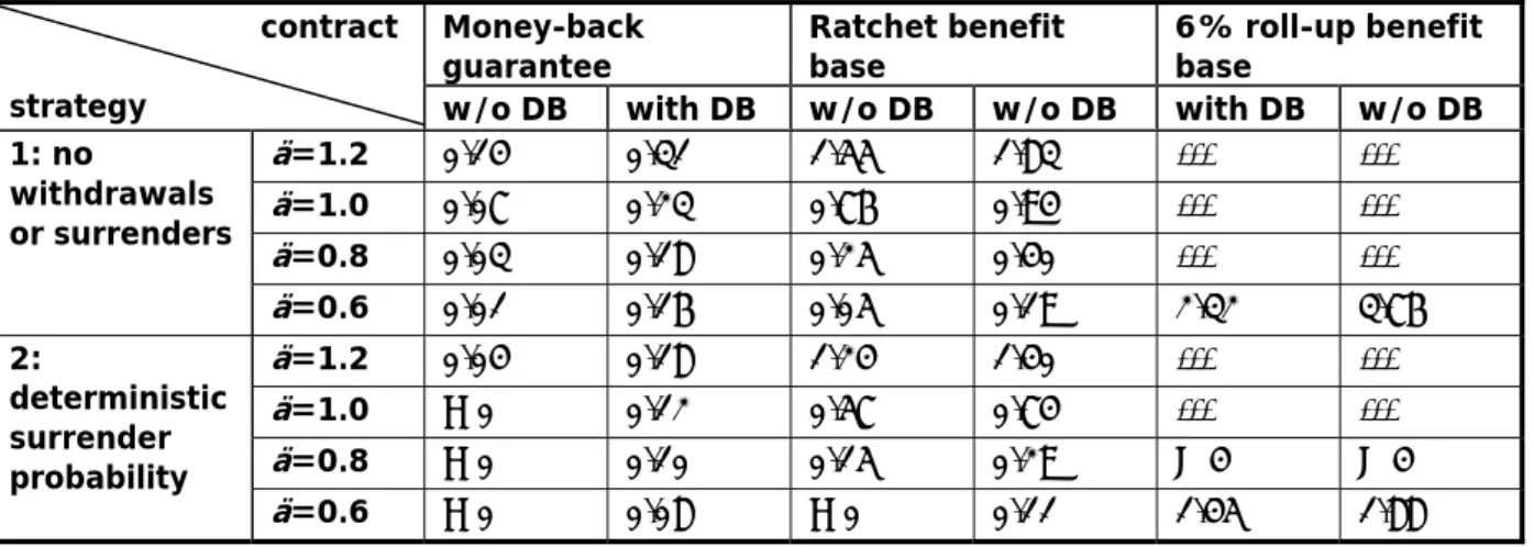
We analyze three different GMIB-contracts for different values of ä. Again, the minimum benefit base for contract 1 is the single premium, contract 2 includes an annual ratchet guarantee whereas contract 3 comes with a 6% roll-up benefit base. The three contracts are analyzed with and without the additional GMDB option from the previous Section. The respective fair guarantee fees are shown in Table 3.

Money-back

guarantee Ratchet benefit base 6% roll-up benefit base contract

strategy w/o DB with DB w/o DB w/o DB with DB w/o DB ä=1.2 0.14% 0.31% 1.55% 1.83% --- --- ä=1.0 0.07% 0.23% 0.76% 0.94% --- --- ä=0.8 0.03% 0.18% 0.25% 0.40% --- --- 1: no withdrawals or surrenders ä=0.6 0.01% 0.16% 0.05% 0.19% 2.32% 3.76% ä=1.2 0.04% 0.18% 1.24% 1.40% --- --- ä=1.0 < 0% 0.12% 0.57% 0.74% --- --- ä=0.8 < 0% 0.10% 0.15% 0.29% > 4% > 4% 2: deterministic surrender probability ä=0.6 < 0% 0.08% < 0% 0.11% 1.45% 1.88%

Table 3: Fair guarantee fee for contracts with GMIB under different consumer behavior Obviously, for , the fair guarantee fees are the same as for the corresponding GMAB options. The value of the guarantee highly depends on the value of ä. Since best estimates about future mortality rates are subject to high uncertainty, this assumption bears a significant risk for the insurer that cannot be hedged with existing financial instruments.

1

= ä

The difference between the fair guarantee fee with or without surrender is huge. Thus, basing the product calculation on estimates about future policyholder behavior bears a significant non-diversifiable risk for the insurer.

For any ä, the values of the three contract types differ considerable. Under strategy 1, there is no fair guarantee fee for a contract with 6% roll-up guarantee for ä ≥ 0.8, i.e. the expected present value of the guaranteed annuities exceeds the single premium. For , the fair guarantee fee equals 2.32% and is much higher than typical charges for these options in the market. Even under strategy 2, the fair guarantee fee is about twice as high as the option price observed in the market. Thus, there is evidence that insurers base their calculations not only on the assumption of irrational surrender behavior. They may also assume other irrationalities, e.g. that policyholders take the lump sum payment (i.e. the account value without guarantee) even if the annuitization option is in the money.

6 . 0

= ä

For the reason described in Section 5.2.2, there is almost no difference between rational policyholder behavior and strategy 1 for contracts with a money-back or a ratchet guarantee. However, in the case of a 6% roll-up benefit base, rational policyholder behavior increases the fair guarantee fee from 2.32% to over 4%. Thus, there have to be many scenarios, where it is optimal to surrender the contract, i.e. the expected present value of future guarantee fees exceeds the value of the option plus the surrender fee.

5.2.4 Contracts with a GMWB Option

In this Section, we analyze a contract with a GMWB option where the initial premium is guaranteed for withdrawals during the life of the contract. The maximum guaranteed annual withdrawal amount is 7% of the initial premium. We analyze this contract with and without a GMDB option (6% roll-up). The third contract considered includes a GMWB with a step-up feature: The total withdrawal amount is increased by 10% after year 5 and 10, respectively, if no withdrawals have occurred until then.

We assume the following policyholder behavior: Under strategy 1, the policyholder withdraws 7% of the initial premium for 14 years starting with year j and surrenders the contract thereafter. For the contract without step-up, we let j=1 while we admit j=1, j=6 and j=11 for the contract with step-up, i.e. the policyholder starts withdrawing immediately after the start of the contract or immediately after a step-up date. Of course, if withdrawals start in the first year, there is no difference between the contracts with and without step-up. In addition we consider the following stochastic customer strategy: The policyholder withdraws 7% of the initial premium if and only if the fund value is lower than the remaining total guaranteed amount of withdrawals, i.e. if . Once , the contract is surrendered. This might be a strategy of a policyholder who tries to intuitively increase the value of the policy without using financial mathematics.

W t t G A < W =0 t G

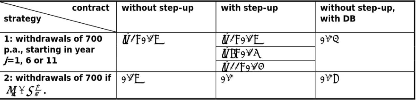
The fair guarantee fees for these contracts are shown in Table 4. contract

strategy without step-up with step-up without step-up, with DB

j=1: 0.19% j=6: 0.15%

1: withdrawals of 700 p.a., starting in year j=1, 6 or 11 j=1: 0.19% j=11: 0.14% 0.23% 2: withdrawals of 700 if . W t t G A < 0.19% 0.2% 0.28%

Table 4: Fair guarantee fee for contracts with GMWB under different consumer behavior The difference between the two strategies is rather small. Furthermore, the results for j=6 and j=11 show that it is not a reasonable strategy to wait with early redemptions until a step-up happens. Of course, this may be different if the guaranteed amount is increased by more than 10% at a step-up date.

The additional fee for including a GMDB option is significantly lower than for the GMAB and GMIB contracts, because every withdrawal leads to a reduction of the guaranteed death benefit. Since strategy 2 results in fewer withdrawals, the additional GMDB fee is slightly higher in this case.

The fair guarantee fees shown are lower than the prices of these guarantees in the market. However, for GMWB options, the fair guarantee fee under rational consumer behavior

increases significantly since there are a variety of options for the customer over the term of the contract. Optimal strategies can not be easily described since they are path-dependent. Without step-ups, the fair guarantee fee assuming rational consumer behavior is more than twice as high as under the above strategies. Milevsky and Salisbury (2006) calculate even higher guarantee fees using a surrender fee of s=1% (compared to 5% in our case). Further analyses showed that reducing the surrender fee in our model significantly raises the fair guarantee fee. For a surrender fee of 0, the fair guarantee fee even exceeds 1%.

Finally, we analyze the influence of the annual maximum guaranteed withdrawal amount on the fair guarantee fee for the contract without step-up. We allow for annual withdrawal amounts of xW=5%, xW=7%, and xW=9%. The fair guarantee fees are displayed in Table 5.

contract

strategy xW

=5% xW =7% xW =9%

1: withdrawals of 700

p.a., starting in year j=1 0.05% 0.19%% 0.38%

Table 5: Influence of the annual maximum free withdrawal amount on the fair guarantee fee for a contract with GMWB

Although the guaranteed total withdrawal amount remains unchanged, the annual maximum withdrawal amount notably influences the fair guarantee fee. Rather low annual redemptions lead to a fair guarantee fee of only 0.05% while a fee of 0.38% is necessary to back a GMWB option with 9% annual withdrawals.

5.3

Sensitivity Analyzes with respect to Capital Marke