ADAPTIVE LIFTING BASED IMAGE COMPRESSION SCHEME WITH PARTICLE SWARM OPTIMIZATION TECHNIQUE

(1)

ADAPTIVE LIFTING BASED IMAGE

COMPRESSION SCHEME WITH

PARTICLE SWARM OPTIMIZATION

TECHNIQUE

1_{Nishat kanvel}

_,

_{Research Scholar(Anna University,Chennai),Lecturer,Dept. of ECE,Thanthai periyar}_{Govt.Institute} ofTechnology,Vellore.

2_{Dr.S.Letitia,Assistant Professor}

_,

_{Dept. of ECE,Thanthai periyar Govt.Institute of Technology,Vellore.}

3_{Dr.Elwin Chandra Monie}

_,

_{Principal,RMK Engineering College,Kaverapettai,Chennai.}

ABSTRACT :This paper presents an adaptive lifting scheme with Particle Swarm Optimization technique for image compression. Particle swarm Optimization technique is used to improve the accuracy of the prediction function used in the lifting scheme. This scheme is applied in Image compression and parameters such as PSNR, Compression Ratio and the visual quality of the image is calculated .The proposed scheme is compared with the existing methods.

1. INTRODUCTION : The wavelet coding method has been recognized as an efficient coding technique for lossy image compression. The wavelet transform decomposes a typical image data to a few coefficients with large magnitude and many coefficients with small magnitude. Since most of the energy of the image concentrates on these coefficients with large magnitude, lossy compression systems just by using coefficients with large magnitude can realize both high compression ratio and the reconstructed image with good quality at the same time. Lifting Scheme (LS) [1,2,3,4] allows efficient construction of the filter banks for wavelet transforms. The limitation of this structure is that the filter structure is fixed over the entire signal. In many applications it is very much desirable to design the filter banks to shape itself to the signal. Several such adaptive Lifting schemes were proposed earlier which consider local characteristics of the signal for adapting. Claypole et al [5] introduced a technique of adaptive filtering which enables to choose the Prediction operators according to the local properties of the image. Boulgouris et al [6] proposed a method of defining lifting operators by constraining the sum of coefficients and by reducing the variance of the signal. A.Gouze et al [7] adapted the lifting method without any a priori model of the image autocovaiance. This method optimizes the update lifting step in order to minimize the distortion. In this paper we propose a new method to obtain wavelet transforms for application in image compression. We have considered a method of changing prediction functions of the LS for each image to improve the compression ratio, gaining a more accurate prediction of pixels in the image. The goal of this paper is to propose an adaptive LS using the Particle Swarm Optimization (PSO) algorithm. Specifically, PSO is used to improve the accuracy of the prediction functions in LS. The proposed method exhibits better accuracy in prediction and can reduce the entropy better than the conventional prediction function on the average.

2.2 PROCEDURE OF LIFTING

The procedure of LS consists of three steps: Split, Predict and Update (Fig. 1)and the inverse lifting scheme is shown in Fig:2

Split: Split the signal into two disjoint subsets of samples. We divide the original signal x[n] into even and odd components: xe[n] and xo[n], where xe[n] = x[2n] and xo[n]= x[2n+1].

Predict: Generate the detail signals d[n] as the prediction error using a prediction operator P:

(2)

Fig 1: Lifting scheme

Fig 2 : Inverse Lifting scheme

Update: Generate the coarser signals c[n] by applying an update operator U to d[n] and adding the result to xe[n]: c[n] xe[n] U(d[n]) (2)

This represents a coarse approximation to the original signal x[n]. These three operations can be applied to c[n] repeatedly. we can easily obtain the inverse lifting scheme of any combination of prediction P and update U. From the equation (1) and (2), xe[n] and xo[n] can be calculated from c[n] and d[n] as shown in the next equations: xo [n] d[n] P(xe[n]) (3)

xe [n] c[n] -U(d[n]) (4)

2.3 LIFTING SCHEME ON TWO DIMENSIONAL IMAGE DATA

When LS transforms the two dimensional data, the procedure explained in the previous subsection is applied two times. At the first step, each row of the image is transformed and divided into two sub images, the sets of {c[n]} and {d[n]}. Secondly, each sub image is scanned vertically, and their columns are transformed similarly. As a result, the original image data is divided into four sub images, cc, cd, dc and dd. The sub image cc can be repeatedly transformed by LS, and this repetition is called multi-resolution analysis.

Since the conventional LS is based on one dimensional signal processing, it does not make good use of two dimensional signals such as image data. That is, at the prediction of the pixels in xo[n], only the pixels in xe[n] on

the same line are allowed to be used in the prediction function The configuration of reference pixels of typical LS is illustrated in Fig. 3, in which xom[n]and xe m[n ]indicate the pixels at the odd and even positions in the mth line of

the image data, and the hatched pixels are allowed to be referred for predicting xo m[n].In the case of the most simple

prediction, the pixel xem[n] and xe m[n 1] are used for predicting xom[n]. Generally, it would seem that the large

number of reference pixels leads to the more accurate prediction, but, xem [n- 1] and xem[n 2] the second closest pixels

from, xom [n] don't contribute to the accurate prediction so much, because they are too distant from xom[n]to correlate

with it strongly. To overcome the difficulty, the proposed method arranges the reference pixels in two dimensional configurations as shown in the Fig.4. The additional reference pixels,

x e m-1 [n], xe m-1 [n+1], xe m+1 [n], xem+1 [n+1]

are expected to correlate with xom[n]better than xem [n- 1] and xem[n 2], because they are closer to xom[n].Using the

(3)

(5)

where pk,l are the coefficients.

xem [n- 1] xem[n] x om[n] xem[n+1] xem[n 2]

Fig 3 : Configuration of reference pixels of conventional lifting scheme

x e m-1 [n] xem-1 [n+1]

xem [n] xmo[n] xem [n+1]

x e m+1 [n] xem+1 [n+1]

Figure 4: Two dimensional configuration of reference pixels

3.2 GROUPING OF PIXEL PATTERNS

The proposed method employs different prediction functions according to the pixel patterns neighboring the target pixels. We assume that the relations between coefficients in Figure 4 are defined as:

p0,0 = p0,1

p1,0 = p1,0= p-1,1=p1,1

In these equations, p0,0 is the only variable and the other coefficients are calculated using it as follows:

. p0,1 =p0,0

p-1,0 = p1,0 = p-1,1=p1,1 = (7)

These are the basic relations between the coefficients, but we cannot use it at the boundaries of the image, because not all reference pixels are available. Then, some different prediction functions are prepared, and one of them is selected according to the positional relation between xom[n]and the boundaries. To improve the accuracy

more, we change the coefficient p0,0 according to the patterns of pixel values.

3.3 OPTIMIZING THE PREDICTION FUNCTION WITH PSO ALGORITHM

In this paper, we focus on the function P defined in (1). Finding suitable P can be taken as an optimization problem to find the optimum values of coefficients in (5). PSO is well suited to solve this problem [8,9,10]. PSO is inspired by flocks of birds or shoals of fish. In PSO a group of particles are placed in the parameter space of problem or function. The algorithm then searches for optima through a series of iterations. The particle’s fitness value is evaluated in each iteration. If it is the best value the particle has achieved, the particle stores the location of that value as pbest (particle best). The location of the best fitness value achieved by any particle during any iteration stored as gbest (global best). Using pbest and gbest, each particle moves with a certain velocity, calculated by (8),(9), and (10).

Vi= wVi−1 + c1 *rand( ) *(pbest − pL)+ c2 *rand( ) *(gbest − pL) (8)

pL = pvL + Vi (9) w = (10)

Viis the current velocity, Vi−1 is the previous velocity, pL is the present location of the particle, pvL is the previous

location of the particle, rnd is a random number between (0, 1), c1 and c2 are learning factors or stochastic factors,

(4)

For each particle

Initialize particle

Calculate fitness value

If the fitness value is better than the best fitness value (pbest) in history

set current value as the new pbest

End

Choose the particle with the best fitness value of all

the particles as the gbest

Calculate particle velocity according to (4) Update particle position according to (5)

End

Continue while maximum iterations

Fig.5 : The Pseudo code of the PSO procedure

The pseudo code of the PSO procedure is presented in Fig.5

The following combinations of the control parameters are used for running PSO. The number of particles is 30. Dimension of particles is four since the parameters need to be tuned are 4. Range of particles is the positive real numbers. The maximum change one particle can take during one iteration is 20. Learning factors or acceleration constants are equal to 1.3. The searching is a repeat process and the stop condition or the maximum number of iterations the PSO executes is set to 200. Inertia weight is set at 0.6 and 0.9, pbest and gbest are equal to 10 . Using the above control parameters, the PSO is executed and the results are obtained.

4. EXPERIMENTAL RESULTS

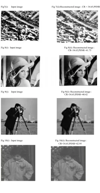
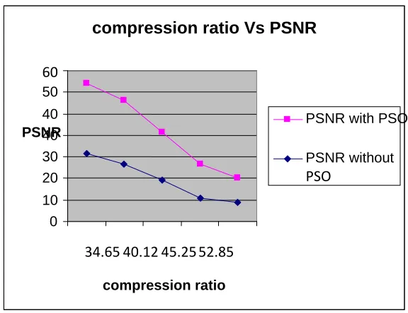
: In this section, the proposed PSO-based lifting Method is simulated and

verified. The following images of size 512 x 512 is used: Girl, Lena,City, Camera man, Child and Zebra images and is shown in Fig. Fig 6(i) 6(ii),7(i)7(ii), 8(i) 8(ii),9(i) 9(ii), 10(i) 10(ii), 11(i)11(ii). The PSNR is found to be high when compared to traditional methods. The encoding and decoding time is also less when PSO is used. Therefore the computational complexity is improved when compared to traditional methods.The convergence process is shown in Fig12 in which particle position verses particle # is converged and Gbest value is calculated which is equal to 254.The gbestvalue vs epoch graph is also drawn. Fig 13. shows PSNR vs CR plot with pso and without pso. Fig6(i) : Input image Fig6(ii) : Reconstructed image :

(5)

Fig7(i): Input image Fig 7(ii):Reconstructed image : CR = 34.65,PSNR=42.15

Fig 8(i): Input image Fig 8(ii): Reconstructed image : CR=34.65,PSNR=41.75

Fig 9(i): Input image Fig 9(ii): Reconstructed image : CR=34.65,PSNR=40.42

Fig 10(i) : Input image Fig 10(ii): Reconstructed image : CR=34.65,PSNR=42.95

(6)

Fig 11(i) : Input image Fig 11(ii) : Reconstructed image: CR=34.65,PSNR=40.75

0 5 10 15 20 25

-60 -40 -20 0

particle #

p

o

s

it

io

n

0 5 10 15 20 25 30

101

102

103

104

epoch

Gbe

s

t v

a

lu

e

PSO: 1 dimensional prob search, Gbestval=254

Fig : 12 Convergence process of L e n a image

Fig 13 : PSNR VS CR graph

_{compression ratio Vs PSNR}

0 10 20 30 40 40 50

60

34.65 40.12 45.25 52.85

compression ratio

PSNR PSNR with PSO

PSNR without

(7)

Table 1: CR and PSNR for Girl image

Compressio n

Ratio

With Particle swarm optimization

Technique Without Particle swarm optimization Technique

PSNR Encodin_{g time} Decodin_{g time} PSNR Encoding _time Decoding _time

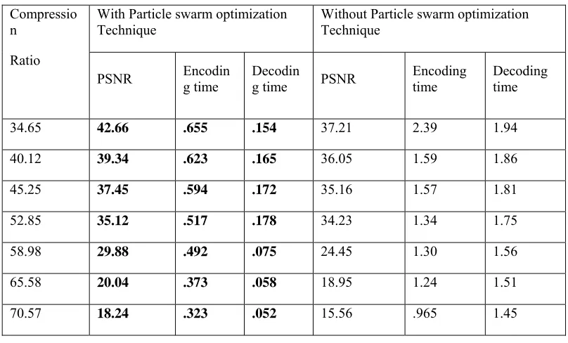
34.65 42.66 .655 .154 37.21 2.39 1.94

40.12 39.34 .623 .165 36.05 1.59 1.86

45.25 37.45 .594 .172 35.16 1.57 1.81

52.85 35.12 .517 .178 34.23 1.34 1.75

58.98 29.88 .492 .075 24.45 1.30 1.56

65.58 20.04 .373 .058 18.95 1.24 1.51

70.57 18.24 .323 .052 15.56 .965 1.45

Table 2 : CR and PSNR for Lena image

Comp ressio n Ratio

Technique Without Particle swarm optimization Technique

PSNR Encoding _time Decoding _time PSNR Encodin_{g time} Decoding _time

34.65 41.75 .635 .153 36.45 2.37 1.92

40.12 40.14 .613 .145 35.75 1.49 1.83

45.25 38.32 .592 .143 35.23 1.43 1.80

52.85 36.03 .509 .151 34.45 1.31 1.69

58.98 30.34 .482 .072 24.12 1.23 1.52

65.58 24.12 .364 .054 18.25 1.19 1.47

(8)

Table 3 : CR and PSNR for city image

Comp ressio n Ratio

Technique Without Particle swarm optimization Technique PSNR Encoding _time Decoding _time PSNR Encodin_{g time} Decoding _time

34.65 42.15 .631 .152 37.25 2.32 1.91

40.12 41.74 .617 .141 36.35 1.47 1.78

45.25 40.32 .591 .139 35.83 1.42 1.75

52.85 39.53 .576 .131 34.95 1.28 1.64

58.98 38.56 .532 .123 27.42 1.21 1.61

65.58 25.21 .461 .053 20.45 1.12 1.42

70.57 20.74 .395 .046 16.34 .947 1.38

Table 4 : : CR and PSNR for cameraman image

Comp ressio n Ratio

With Particle swarm optimization Technique

Without Particle swarm optimization Technique

PSNR Encoding _time Decoding _time PSNR Encodin_{g time} Decoding _time

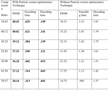
34.65 40.42 .629 .149 34.15 2.13 1.91

40.12 40.02 .621 .141 33.25 1.47 1.79

45.25 39.12 .584 .139 32.13 1.42 1.75

52.85 37.53 .549 .121 31.95 1.30 1.61

58.98 36.24 .442 .032 23.32 1.21 1.51

65.58 27.12 .314 .043 17.55 1.12 1.42

(9)

Table 5 : CR and PSNR for child image

Compr ession Ratio

PSNR

Encoding time

Decoding

time PSNR

Encoding time

Decoding time

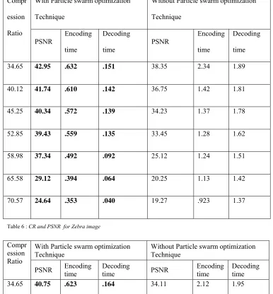
34.65 42.95 .632 .151 38.35 2.34 1.89

40.12 41.74 .610 .142 36.75 1.42 1.81

45.25 40.34 .572 .139 34.23 1.37 1.78

52.85 39.43 .559 .135 33.45 1.28 1.62

58.98 37.34 .492 .092 25.12 1.24 1.51

65.58 29.12 .394 .064 20.25 1.13 1.42

70.57 24.64 .353 .040 19.27 .923 1.37

Table 6 : CR and PSNR for Zebra image

Compr ession Ratio

PSNR Encoding _time Decoding _time PSNR Encoding _time Decoding _time

34.65 40.75 .623 .164 34.11 2.12 1.95

40.12 39.72 .617 .156 33.23 1.42 1.76

45.25 39.02 .581 .145 31.75 1.39 1.73

52.85 36.53 .543 .137 30.93 1.33 1.60

58.98 34.42 .424 .113 21.32 1.25 1.55

65.58 25.32 .306 .109 16.65 1.17 1.46

(10)

5. Inference:

In this paper the prediction function is optimized using PSO. This is being tested on various images. We e v a l u a t e t h e performance o f the presented scheme. We used standard test grayscale images for the evaluation. The results are shown from Table 1 to Table 6. It is interesting that Lena image, Girl image, City image and Child image have good visual quality because there are no sharp edges in the image when compared to Camera man image and Zebra image.

6. Conclusion:

In this paper we propose a method to optimize the prediction function used in the lifting scheme using Particle swarm optimization algorithm (PSO) for image compression. Since in PSO, there are only few parameters to deal with, it is efficient. Large numbers of processing elements, so called dimensions, enable to reach the solution space effectively. It also converges to a solution very quickly which is a desirable property in combinatorial optimization problems. Results of the proposed method are good when compared to existing methods in terms of compression ratio, PSNR, encoding time, decoding time. The computational complexity is also reduced as PSO is used. The quality of the reconstructed image is promising when compared to existing methods.

References

[1] W. Sweldens, “The lifting scheme: A new philosophy in biorthogonal wavelet constructions”, in Proc. SPIE, vol. 2569,1995, pp. 68–79.

[2] A. R. Calderbank, I. Daubechies,W. Sweldens, and B.-L. Yeo, “Wavelet transforms that map integers to integers”, J. Appl. Comput. Harmon. Anal., vol. 5, no. 3, 1998.

[3] W. Sweldens, “The lifting scheme: A construction of second- generation wavelets”, SIAM J. Math. Anal., vol. 29, no. 2, pp. 511– 546, 1997.

[4] M. Adams and F. Kossentini, “Reversible Integer-to-Integer Wavelet Transforms for Image Compression: Performance Evaluation and Analysis”, IEEE Trans. on Image Processing, vol.9, no. 6, pp. 1010-1024, Jun. 2000.

[5] R.L. Claypoole,G.M. Davies, W.Sweldens and R.G. Baraniuk, ‘Non-linear wavelet transforms for image coding via lifting”, IEEE Trans. Image Processing, Vol.12,pp. 1449-1459,Dec. 2003

[6] N. V. Boulgouris, D. Tzovaras, and M. G. Strintzis, “Lossless image compression based on optimal prediction, adaptive lifting, and conditional arithmetic coding”, IEEE Trans. Image Process., vol. 10, no. 1, pp. 1–14, Jan. 2001.

[7] A. Gouze, M. Antonini, M. Barlaud and B. Macq, “Design of signal-Adapted multidimensional lifting scheme for lossy coding, IEEE Trans. Image Processing, Vol. 13, No. 12, pp. 1589-1602, Dec. 2004

[8] J. Kennedy, R. C. Eberhart, and Y.Shi, Swarm Intelligence, Morgan Kaufmann Publishers, San Francisco,2001.

[9] T. J. Richer and T. M. Blackwell, “When is a swarm necessary?,” pp. 5618–5625, Proceedings of IEEE Congress on Evolutionary Computation (CEC2006), Vancouver, BC, Canada, 2006