Survey on deep learning with class imbalance

Survey on deep learning with class

imbalance

Justin M. Johnson

_{and Taghi M. Khoshgoftaar}

Introduction

Supervised learning methods require labeled training data, and in classification prob-lems each data sample belongs to a known class, or category [1, 2]. In a binary classifi-cation problem with data samples from two groups, class imbalance occurs when one class, the minority group, contains significantly fewer samples than the other class, the majority group. In many problems [3–7], the minority group is the class of inter-est, i.e., the positive class. A well-known class imbalanced machine learning scenario is the medical diagnosis task of detecting disease, where the majority of the patients are

Abstract

The purpose of this study is to examine existing deep learning techniques for address-ing class imbalanced data. Effective classification with imbalanced data is an impor-tant area of research, as high class imbalance is naturally inherent in many real-world applications, e.g., fraud detection and cancer detection. Moreover, highly imbalanced data poses added difficulty, as most learners will exhibit bias towards the majority class, and in extreme cases, may ignore the minority class altogether. Class imbalance has been studied thoroughly over the last two decades using traditional machine learning models, i.e. non-deep learning. Despite recent advances in deep learning, along with its increasing popularity, very little empirical work in the area of deep learning with class imbalance exists. Having achieved record-breaking performance results in several complex domains, investigating the use of deep neural networks for problems contain-ing high levels of class imbalance is of great interest. Available studies regardcontain-ing class imbalance and deep learning are surveyed in order to better understand the efficacy of deep learning when applied to class imbalanced data. This survey discusses the imple-mentation details and experimental results for each study, and offers additional insight into their strengths and weaknesses. Several areas of focus include: data complexity, architectures tested, performance interpretation, ease of use, big data application, and generalization to other domains. We have found that research in this area is very limited, that most existing work focuses on computer vision tasks with convolutional neural networks, and that the effects of big data are rarely considered. Several tradi-tional methods for class imbalance, e.g. data sampling and cost-sensitive learning, prove to be applicable in deep learning, while more advanced methods that exploit neural network feature learning abilities show promising results. The survey concludes with a discussion that highlights various gaps in deep learning from class imbalanced data for the purpose of guiding future research.

Keywords: Deep learning, Deep neural networks, Class imbalance, Big data

Open Access

© The Author(s) 2019. This article is distributed under the terms of the Creative Commons Attribution 4.0 International License (http://creat iveco mmons .org/licen ses/by/4.0/), which permits unrestricted use, distribution, and reproduction in any medium, provided you give appropriate credit to the original author(s) and the source, provide a link to the Creative Commons license, and indicate if changes were made.

SURVEY PAPER

healthy and detecting disease is of greater interest. In this example, the majority group of healthy patients is referred to as the negative class. Learning from these imbalanced data sets can be very difficult, especially when working with big data [8, 9], and non-standard machine learning methods are often required to achieve desirable results. A thorough understanding of the class imbalance problem and the methods available for addressing it is indispensible, as such skewed data exists in many real-world applications.

When class imbalance exists within training data, learners will typically over-clas-sify the majority group due to its increased prior probability. As a result, the instances belonging to the minority group are misclassified more often than those belonging to the majority group. Additional issues that arise when training neural networks with imbal-anced data will be discussed in the "Deep learning methods for class imbalanced data" section. These negative effects make it very difficult to accomplish the typical objective of accurately predicting the positive class of interest. Furthermore, some evaluation met-rics, such as accuracy, may mislead the analyst with high scores that incorrectly indi-cate good performance. Given a binary data set with a positive class distribution of 1%, a naïve learner that always outputs the negative class label for all inputs will achieve 99% accuracy. Many traditional machine learning techniques, which are summarized in the "Machine learning techniques for class imbalanced data" section, have been devel-oped over the years to combat these adverse effects.

Methods for handling class imbalance in machine learning can be grouped into three categories: data-level techniques, algorithm-level methods, and hybrid approaches [10]. Data-level techniques attempt to reduce the level of imbalance through various data sampling methods. Algorithm-level methods for handling class imbalance, commonly implemented with a weight or cost schema, include modifying the underlying learner or its output in order to reduce bias towards the majority group. Finally, hybrid systems strategically combine both sampling and algorithmic methods [10].

Over the last 10 years, deep learning methods have grown in popularity as they have improved the state-of-the-art in speech recognition, computer vision, and other domains [11]. Their recent success can be attributed to an increased availability of data, improve-ments in hardware and software [12–16], and various algorithmic breakthroughs that speed up training and improve generalization to new data [17]. Despite these advances, very little statistical work has been done which properly evaluates techniques for han-dling class imbalance using deep learning and their corresponding architectures, i.e. deep neural networks (DNNs). In fact, many researchers agree that the subject of deep learning with class imbalanced data is understudied [18–23]. For this reason, our survey is limited to just 15 deep learning methods for addressing class imbalance.

not demonstrate learning from class imbalanced data with neural networks containing two or more hidden layers. No restrictions were placed on the date of publication. The matched search results were then used to perform backward and forward searches, i.e. reviewing the references of matched articles and additional sources that have cited these articles. This was repeated until all relevant papers were identified, to the best of our knowledge.

Additional selection criteria were applied to exclude papers that only tested low lev-els of class imbalance, that did not compare proposed methods to other existing class imbalance methods, or that only used a single data set for evaluation. We discovered that papers meeting these criteria are very limited. Therefore, in order to increase the total number of selected works, these additional requirements were relaxed. The final set of 15 publications includes journal articles, conference papers, and student theses that employ deep learning methods with class imbalanced data.

We explore a variety of data-level, algorithm-level, and hybrid deep learning meth-ods designed to improve the classification of imbalanced data. Implementation details, experimental results, data set details, network topologies, class imbalance levels, perfor-mance metrics, and any known limitations are included in each surveyed work’s discus-sion. Tables 17 and 18, in the "Discussion of surveyed works" section, summarize all of the surveyed deep learning methods and the details of their corresponding data sets. This survey provides the most current analysis of deep learning methods for addressing class imbalance, summarizing and comparing all related work to date, to the best of our knowledge.

The remainder of this paper is organized as follows. The "Class imbalance background" section provides background information on the class imbalance problem, reviews per-formance metrics that are more sensitive to class imbalanced data, and discusses some of the more popular traditional machine learning (non-deep learning) techniques for handling imbalanced data. The  "Deep learning background" section provides neces-sary background information on deep learning. The neural network architectures used throughout the survey are introduced, along with several important milestones and the use of deep learning in solving big data analytics challenges. The "Deep learning meth-ods for class imbalanced data" section surveys 15 published studies that analyze deep learning methods for addressing class imbalance. The  "Discussion of surveyed works" section summarizes the surveyed works and offers further insight into their various strengths and weaknesses. The "Conclusion" section concludes the survey and discusses potential areas for future work.

Class imbalance background

The class imbalance problem

Skewed data distributions naturally arise in many applications where the positive class occurs with reduced frequency, including data found in disease diagnosis [3], fraud detection [4, 5], computer security [6], and image recognition [7]. Intrinsic imbalance is the result of naturally occurring frequencies of data, e.g. medical diagnoses where the majority of patients are healthy. Extrinsic imbalance, on the other hand, is introduced through external factors, e.g. collection or storage procedures [28].

It is important to consider the representation of the minority and majority classes when learning from imbalanced data. It was suggested by Krawczyk [10] that good results can be obtained, regardless of class disproportion, if both groups are well rep-resented and come from non-overlapping distributions. Japkowicz [29] examined the effects of class imbalance by creating artificial data sets with various combinations of complexity, training set size, and degrees of imbalance. The results show that sensitivity to imbalance increases as problem complexity increases, and that non-complex, linearly separable problems are unaffected by all levels of class imbalance.

In some domains, there is a genuine lack of data due to the low frequency with which events occur, e.g. detecting oil spills [7]. Learning from extreme class imbalanced data, where the minority class accounts for as few as 0.1% of the training data [10, 30], is of great importance because it is typically these rare occurrences that we are most inter-ested in. Weiss [31] discusses the difficulties of learning from rare events and various machine learning techniques for addressing these challenges.

The total number of minority samples available is of greater interest than the ratio or percentage of the minority. Consider a minority group that is just 1% of a data set con-taining 1 million samples. Regardless of the high level of imbalance, there are still many positive samples (10,000) available to train a model. On the other hand, an imbalanced data set where the minority class displays rarity or under-representation is more likely to compromise the performance of the classifier [30].

For the purpose of comparing experimental results across all works presented in this survey, a ratio ρ (Eq. 1) [23] will be used to indicate the maximum between-class imbal-ance level. Ci is a set of examples in class i, and maxi{|Ci|} and mini{|Ci|} return the max-imum and minmax-imum class size over all i classes, respectively. For example, if a data set’s largest class has 100 samples and its smallest class has 10 samples, then the data has an imbalance ratio of ρ₌10 . Since the actual number of samples may prove more impor-tant than the ratio, Table 18 also includes the maximum and minimum class sizes for all experiments in this survey.

Performance metrics

The confusion matrix in Table 1 summarizes binary classification results. The FP and FN errors correspond to Type I and Type II errors, respectively. All of the performance met-rics listed in this section can be derived from the confusion matrix.

(1) ρ₌ maxi{|Ci|}

Accuracy (Eq. 2) and error rate (Eq. 3) are the most frequently used metrics when evalu-ating classification results. When working with class imbalance, however, both are insuf-ficient, as the resulting value is dominated by the majority group, i.e. the negative class. As mentioned previously, when given a data set whose positive group distribution is just 1% of the data set, a naïve classifier can achieve a 99% accuracy score by simply labeling all examples as negative. Of course, such a model would provide no real value. For this reason, we review several popular evaluation metrics commonly used with imbalanced data problems.

Precision (Eq. 4) measures the percentage of the positively labeled samples that are actu-ally positive. Precision is sensitive to class imbalance because it considers the number of negative samples incorrectly labeled as positive. Precision alone is insufficient, however, because it provides no insight into the number of samples from the positive group that were mislabeled as negative. On the other hand, Recall (Eq. 5), or the True Positive Rate (TPR), measures the percentage of the positive group that was correctly predicted to be positive by the model. Recall is not affected by imbalance because it is only depend-ent on the positive group. Recall does not consider the number of negative samples that are misclassified as positive, which can be problematic in problems containing class imbalanced data with many negative samples. There is a trade-off between precision and recall, and the metric of greater importance varies from problem to problem. Selectivity (Eq. 6), or the True Negative Rate (TNR), measures the percentage of the negative group that was correctly predicted to be negative.

(2)

Accuracy= TP+TN

TP₊TN₊FP₊FN

(3)

Error Rate= 1−Accuracy

(4) Precision₌ TP

TP+FP

(5) Recall=TPR= TP

TP+FN

(6)

Selectivity₌TNR₌ TN TN+FP

(7) F-Measure=(1+β

2_{)×Recall×Precision}

β2_×Recall₊Precision

(8) G-Mean=√TPR×TNR

(9) Balanced Accuracy₌1

2×(TPR+TNR) Table 1 Confusion matrix

Actual positive Actual negative

The F-Measure (Eq. 7), or F1-score, combines precision and recall using the harmonic mean, where coefficient β is used to adjust the relative importance of precision versus recall. The G-Mean (Eq. 8) measures performance by combining both the TPR and the TNR metrics using the square root of their product. Similar to the G-Mean, the Bal-anced Accuracy (Eq. 9) metric also combines TPR and TNR values to compute a metric that is more sensitive to the minority group [18]. Although F-Measure, G-Mean, and Balanced Accuracy are improvements over Accuracy and Error Rate, they are still not entirely effective when comparing performance between classifiers and various distribu-tions [28].

The receiver operating characteristics (ROC) curve, first presented by Provost and Faw-cett [32], is another popular assessment which plots true positive rate over false posi-tive rate, creating a visualization that depicts the trade-off between correctly classified positive samples and incorrectly classified negative samples. For models which produce continuous probabilities, thresholding can be used to create a series of points along ROC space [28]. From this a single summary metric, the area under the ROC curve (AUC), can be computed and is often used to compare performance between models. A weighted-AUC metric, which takes cost biases into consideration when calculating the area, was introduced by Weng and Poon [33].

According to Davis and Goadrich [34], ROC curves can present overly optimis-tic results on highly skewed data sets and Precision–Recall (PR) curves should be used instead. The authors claim that a curve can only dominate in ROC space if it also domi-nates in PR space. This is justified by the fact that the false positive rate used by ROC,

FPR_{= FP+TN}FP , will be less sensitive to changes in FP as the size of the negative class

grows.

According to Seliya et al. [35], learners should be evaluated with a set of complemen-tary performance metrics, where each individual metric captures a different aspect of performance. In their comprehensive study, 22 different performance metrics were used to evaluate two classifiers across 35 unique data sets. Common factor analysis was then used to group the metrics, identifying sets of unrelated performance metrics that can be used in tandem to reduce redundancy and improve performance interpretation. One example set of complementary performance metrics discovered by Seliya et al. is AUC, Brier Inaccuracy [36], and accuracy.

Machine learning techniques for class imbalanced data

Data‑level methods

Data-level methods for addressing class imbalance include over-sampling and under-sampling. These techniques modify the training distributions in order to decrease the level of imbalance or reduce noise, e.g. mislabeled samples or anomalies. In their sim-plest forms, random under-sampling (RUS) discards random samples from the majority group, while random over-sampling (ROS) duplicates random samples from the minor-ity group [37].

Under-sampling voluntarily discards data, reducing the total amount of information the model has to learn from. Over-sampling will cause an increased training time due to the increased size of the training set, and has also been shown to cause over-fitting [38]. Over-fitting, characterized by high variance, occurs when a model fits too closely to the training data and is then unable to generalize to new data. A variety of intelligent sam-pling methods have been developed in an attempt to balance these trade-offs.

Intelligent under-sampling methods aim to preserve valuable information for learning. Zhang and Mani [39] present several Near-Miss algorithms that use a K-nearest neigh-bors (K-NN) classifier to select majority samples for removal based on their distance from minority samples. One-sided selection was proposed by Kubat and Matwin [40] as a method for removing noisy and redundant samples from the majority class as they are discovered through a 1-NN rule and Tomek links [41]. Barandela et al. [42] use Wilson’s editing [43], a K-NN rule that removes misclassified samples from the training set, to remove majority samples from class boundaries.

A number of informed over-sampling techniques have also been developed to strengthen class boundaries, reduce over-fitting, and improve discrimination. Chawla et  al. [44] introduced the Synthetic Minority Over-sampling Technique (SMOTE), a method that produces artificial minority samples by interpolating between existing minority samples and their nearest minority neighbors. Several variants to SMOTE, e.g. Borderline-SMOTE [45] and Safe-Level-SMOTE [46], improve upon the original algo-rithm by also taking majority class neighbors into consideration. Borderline-SMOTE limits over-sampling to the samples near class borders, while Safe-Level-SMOTE defines safe regions to prevent over-sampling in overlapping or noise regions.

Supervised learning systems usually define a concept with several disjuncts, where each disjunct is a conjunctive definition describing a subconcept [47]. The size of a dis-junct corresponds to the number of samples that the disdis-junct correctly classifies. Small disjuncts, often corresponding to rare cases in the domain, are learned concepts that correctly classify only a few data samples. These small disjuncts are problematic, as they often contain much higher error rates than large disjuncts, and they cannot be removed without compromising performance [48].

Jo and Japkowicz [49] proposed cluster-based over-sampling to address the presence of small disjuncts in the training data. Minority and majority groups are first clustered using the K-means algorithm, then over-sampling is applied to each cluster separately. This improves both within-class imbalance and between-class imbalance.

performance metric. Experiments revealed that RUS resulted in good performance over-all, outperforming ROS and intelligent sampling methods in most cases. The results sug-gest that, although RUS performs well in most cases, no sampling method is guaranteed to perform best in all problem domains, and multiple performance metrics should be used when evaluating results.

Algorithm‑level methods

Unlike data sampling methods, algorithmic methods for handling class imbalance do not alter the training data distribution. Instead, the learning or decision process is adjusted in a way that increases the importance of the positive class. Most commonly, algorithms are modified to take a class penalty or weight into consideration, or the decision thresh-old is shifted in a way that reduces bias towards the negative class.

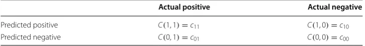
In cost-sensitive learning, penalties are assigned to each class through a cost matrix. Increasing the cost of the minority group is equivalent to increasing its importance, decreasing the likelihood that the learner will incorrectly classify instances from this group [10]. The cost matrix of a binary classification problem is shown in Table 2 [50]. A given entry of the table, cij , is the cost associated with predicting class i when the true

class is j. Usually, the diagonal of the cost matrix, where i=j , is set to 0. The costs

corre-sponding to false positive and false negative errors are then adjusted for desired results. Ling and Sheng [51] categorize cost-sensitive methods as either a direct method, or a meta-learning method. Direct methods are methods that have cost-sensitive capabilities within themselves, achieved through modification of the learner’s underlying algorithm such that costs are taken into consideration during learning. The optimization process changes from one of minimizing total error, to one of minimizing total cost. Meta-learn-ing methods utilize a wrapper to convert cost-insensitive learners into cost-sensitive systems. If a cost-insensitive classifier produces posterior probability estimates, the cost matrix can be used to define a new threshold p∗ such that:

Usually, thresholding methods use p∗ (Eq. 10) to redefine the output decision threshold

when classifying samples [51]. Threshold moving, or post-processing the output class probabilities using Eq. 10, is one meta-learning approach that converts a cost-insensitive learner into a cost-sensitive system.

One of the biggest challenges in cost-sensitive learning is the assignment of an effec-tive cost matrix. The cost matrix can be defined empirically, based on past experiences, or a domain expert with knowledge of the problem can define them. Alternatively, the false negative cost can be set to a fixed value while the false positive cost is varied, using a validation set to identify the ideal cost matrix. The latter has the advantage of exploring (10) p∗₌ c10

c10+c01

Table 2 Cost matrix

Actual positive Actual negative

Predicted positive C(1, 1)=c11 C(1, 0)=c10

a range of costs, but can be expensive and even impractical if the size of the data set or number of features is too large.

Hybrid methods

Data-level and algorithm-level methods have been combined in various ways and applied to class imbalance problems [10]. One strategy includes performing data sam-pling to reduce class noise and imbalance, and then applying cost-sensitive learning or thresholding to further reduce the bias towards the majority group. Several techniques which combine ensemble methods with sampling and cost-sensitive learning were pre-sented in [28]. Liu et al. [52] proposed two algorithms, EasyEnsemble and BalanceCas-cade, that learn multiple classifiers by combining subsets of the majority group with the minority group, creating pseudo-balanced training sets for each individual classifier. SMOTEBoost [53], DataBoost-IM [54], and JOUS-Boost [55] all combine sampling with ensembles. Sun [56] introduced three cost-sensitive boosting methods, namely AdaC1, AdaC2, and AdaC3. These methods iteratively increase the impact of the minority group by introducing cost items into the AdaBoost algorithm’s weight updates. Sun showed that the cost-sensitive boosted ensembles outperformed plain boosting methods in most cases.

Deep learning background

This section reviews the basic concepts of deep learning, including descriptions of the neural network architectures used throughout the surveyed works and the value of representation learning. We also touch on several important milestones that have con-tributed to the success of deep learning. Finally, the rise of big data analytics and its challenges are introduced along with a discussion on the role of deep learning in solving these challenges.

Introduction to deep learning

Deep learning is a sub-field of machine learning that uses artificial neural networks (ANNs) containing two or more hidden layers to approximate some function f∗ _{, where} f∗ can be used to map input data to new representations or make predictions. The ANN,

inspired by the biological neural network, is a set of interconnected neurons, or nodes, where connections are weighted and each neuron transforms its input into a single out-put by applying a non-linear activation function to the sum of its weighted inout-puts. In a feedforward network, input data propagates through the network in a forward pass, each hidden layer receiving its input from the previous layer’s output, producing a final output that is dependent on the input data, the choice of activation function, and the weight parameters [1]. Gradient descent optimization is then used to adjust the net-work’s weight parameters in order to minimize the loss function, i.e. the error between expected output and actual output.

The convolutional neural network (CNN) is a specialized feedforward neural net-work that was designed to process multi-dimensional data, e.g. images [58]. It was inspired by the brain’s visual cortex and its origins date back to the Neocognitron presented by Fukushima in 1980 [59]. A CNN architecture is typically comprised of convolutional layers, pooling (subsampling) layers, and fully-connected layers. Fig-ure 2 illustrates the LeNet-5 CNN architecture proposed by LeCun et al. [58] in 1998 for the purpose of character recognition. Unlike fully-connected layers, a single unit of a convolutional layer is only connected to a small receptive field of its input, where the weights of its connections define a filter bank [11]. The convolution operation is used to slide the filter bank across the input, producing activations at each recep-tive field that combine to form a feature map [60]. In other words, the same set of weights are used to detect a specific feature, e.g. a horizontal line, at each receptive field of the input, and the output feature map indicates the presence of this feature at each location. The concept of local connections and shared weights take advantage of the fact that input signals in close proximity of each other are usually highly cor-related, and that input signals are often invariant to location. By combining multiple filter banks in a single convolutional layer, the layer can learn to detect multiple fea-tures in the input, and the resulting feature maps become the input of the next layer. Pooling layers are added after one or more convolutional layers in order to merge semantically similar features and reduce dimensionality [11]. After the convolutional and pooling layers, the multi-dimensional output is flattened and fed to fully-con-nected layers for classification. Similar to the MLP, output activations are fed from

Fig. 1 Shallow MLP vs deep MLP [57]

one layer to the next in a forward pass, and the weights are updated through gradi-ent descgradi-ent.

The MLP and CNN are just two of many alternative DNN architectures that have been developed over the years. Recurrent neural networks (RNNs), autoencoders, and stochastic networks are explained thoroughly in [1, 60, 61]. They also present advanced optimization techniques that have been shown to improve training time and performance, e.g. regularization methods, parameter initialization, improved optimizers and activation functions, and normalization techniques.

Representation learning

The success of a conventional machine learning algorithm is highly dependent on the representation of the input data, making feature engineering a critical step in the machine learning workflow. This is very time consuming and for many complex prob-lems, e.g. image recognition, it can be extremely difficult to determine which features will yield the best results. Deep learning offers a solution to this problem by building upon the concept of representation learning [11].

Representation learning is the process of using machine learning to map raw input data features into a new representation, i.e. a new feature space, for the purpose of improving detection and classification tasks. This mapping from raw input data to new representations is achieved through non-linear transformations of the input data. Com-posing multiple non-linear transformations creates hierarchical representations of the input data, increasing the level of abstraction through each transformation. This auto-matic generation of new features saves valuable time by removing the need for experts to manually hand engineer features, and improves overall performance in many complex problem domains, such as image and speech, where it is otherwise difficult to determine the best features. As data passes through the hidden layers of a DNN, it is transformed by each layer into a new representation. Given sufficient data, DNNs are able to learn high-level feature representations of inputs through the composition of multiple hidden layers. These learned representations amplify components of the input which are impor-tant for discrimination, while suppressing those that are unimporimpor-tant [11]. Deep learn-ing architectures achieve their power through this composition of increaslearn-ingly complex abstract representations [60]. This approach to problem solving intuitively makes sense, as composing simple concepts into complex concepts is analogous to many real-world problem domains.

Deep learning milestones

and that systems nearly always reach solutions of similar quality [11]. Despite some early successes in the late 1980s [64] and 1990s [58], DNNs were mostly forsaken in practice and research due to these challenges.

In 2006, interests in deep learning were revived as research groups presented methods for sensibly initializing DNN weights with an unsupervised layer-wise pre-training pro-cedure [65, 66]. These pre-trained Deep Belief Networks (DBNs) can then be efficiently fine-tuned through supervised learning. They proved to be very effective in image and speech tasks, and led to record breaking results on a speech recognition task in 2009 and the deployment of deep learning speech systems in Android mobile devices by 2012 [11].

In 2012, Krizhevsky et al. [17] submitted a deep CNN to the Large Scale Visual Recog-nition Challenge (LSVRC) [67] that nearly halved the top-5% error rate, reducing from the previous year’s 26% down to just 16%. The work by Krizhevsky et al. included several crucial methods which have since become common practice in deep learning work. The CNN was implemented on multiple graphics processing units (GPUs). The drastic speed-up provided by parallel GPU computing allows for the training of deeper networks with larger data sets, and increased research productivity. A new non-saturating activation function, the rectified linear unit (ReLU), alleviated the vanishing gradient problem and allowed for faster training. Dropout was introduced as a regularization method to decrease over fitting in high capacity networks with many layers. Dropout simulates the ensembling of many models by randomly disabling neurons with a probability P∈ [0, 1_]

during each iteration, forcing the model to learn more robust features. Data augmenta-tion, artificially enlarging the data set by applying transformations to data samples, was also applied as a regularization technique. This event marked a major turning point and sparked new interest in deep learning and computer vision.

This newfound interest in deep learning drove leading technological companies to increase research efforts, producing many advances in deep learning and pushing the state-of-the-art in deep learning to new levels. Deep learning frameworks which abstract tensor computation [12–15] and GPU compatibility libraries [16] have been made avail-able to the community through open source software [68] and cloud services [69, 70]. Combined with an increasing amount of available data and public attention, deep learn-ing is growlearn-ing at a faster pace than ever before.

Deep learning with big data

Many organizations are being faced with the challenges of big data, as they are explor-ing large volumes of data to extract value and guide decisions [71]. Big data refers to data which exceeds the capabilities of standard data storage and data processing systems [72]. This forces practitioners to adopt new techniques for storing, manipulating, and analyzing data. The rise of big data can be attributed to improvements in hardware and software, increased internet and social media activity, and a growing abundance of sen-sor-enabled interconnected devices, i.e. the internet of things (IoT).

shown to exacerbate the negative effects of class imbalanced data [74]. Advanced tech-niques for quickly processing incoming data streams and maintaining appropriate turna-round times are required to keep up with the rate at which data is being generated, i.e. data velocity. The variety of big data corresponds to the mostly unstructured, diverse, and inconsistent representations that arise as data is consumed from multiple sources over extended periods of time. This variety further increases the computational com-plexity of data preprocessing and machine learning. Finally, the veracity of big data, i.e. its accuracy and trustworthiness, must be regularly validated to ensure results do not become corrupted by invalid input. Some additional machine learning challenges that are magnified by big data include high-dimensionality, distributed infrastructures, real-time requirements, feature engineering, and data cleansing [75].

Najafabadi et al. [75] discuss the use of deep learning in solving big data challenges. The ability of DNNs to extract meaningful features from large sets of unlabeled data is particularly important, as this is commonly encountered in big data analytics. The auto-matic extraction of features from mostly unstructured and diverse data, e.g. image, text and audio data, is therefore extremely useful. With abstract features extracted from big data through deep learning methods, simple linear models can often be used to com-plete machine learning tasks more efficiently. Advanced semantic-based information storage and retrieval systems, e.g. semantic indexing and hashing [76, 77], are also made possible with these high-level features. In addition, deep learning has been used to tag incoming data streams, helping to group and organize fast-moving data [75]. In general, high-capacity DNNs are well suited for learning from the large volumes of data encoun-tered in big data analytics.

As the presence of big data within organizations continues to increase, new methods will be required to keep up with the influx of data. Despite being relatively immature, deep learning methods are proving effective in solving many big data challenges. We believe that advances in deep learning, especially in learning from unsupervised data, will play a critical role in the future of big data analytics.

Deep learning methods for class imbalanced data

Anand et al. [78] explored the effects of class imbalance on the backpropagation algo-rithm in shallow neural networks in the 1990’s. The authors show that in class imbal-anced scenarios, the length of the minority class’s gradient component is much smaller than the length of the majority class’s gradient component. In other words, the major-ity class is essentially dominating the net gradient that is responsible for updating the model’s weights. This reduces the error of the majority group very quickly during early iterations, but often increases the error of the minority group and causes the network to get stuck in a slow convergence mode.

consistency, class imbalance is presented as the maximum between-class ratio, ρ (Eq. 1), for all surveyed works.

Data‑level methods

This section includes four papers that explore data-level methods for addressing class imbalance with DNNs. Hensman and Masko [79] first show that balancing the training data with ROS can improve the classification of imbalanced image data. Then RUS and augmentation methods are used by Lee et al. [20] to decrease class imbalance for the purpose of pre-training a deep CNN. Pouyanfar et al. [21] introduce a new dynamic sam-pling method that adjusts samsam-pling rates according to class-wise performance. Finally, Buda et al. [23] compare RUS, ROS, and two-phase learning across multiple imbalanced image data sets.

Balancing training data with ROS

Hensman and Masko [79] explored the effects of class imbalance and ROS using deep CNNs. The CIFAR-10 [80] benchmark data set, comprised of 10 classes with 6000 images per class, was used to generate 10 imbalanced data sets for testing. These 10 gen-erated data sets contained varying class sizes, ranging between 6% and 15% of the total data set, producing a max imbalance ratio ρ₌2.3 . In addition to varying the class size,

the different distributions also varied the number of minority classes, where a minority class is any class smaller than the largest class. For example, a major 50–50 split (Dist. 3) reduced five of the classes to 6% of the data set size and increased five of the classes to 14%. As another example, a major singular over-representation (Dist. 5) increased the size of the airplane class to 14.5%, reducing the other nine classes slightly to 9.5%.

A variant of the AlexNet [17] CNN, which has proven to perform well on CIFAR-10, was used for all experiments by Hensman and Masko. The baseline performance was defined by training the CNN on all distributions with no data sampling. The ROS method being evaluated consisted of randomly duplicating samples from the minority classes until all classes in the training set had an equal number of samples.

Hensman and Masko presented their results as the percentage of correct answers per class, and included the mean score for all classes, denoted by Total. To ensure results were valid, a total of three runs were completed for each experiment and then aver-aged. Table 3 shows the results of the CNN without any data sampling. These results demonstrate the impact of class imbalance when training a CNN model. Most of the imbalanced distributions saw a loss in performance. Dist. 6 and Dist. 7, which contained very slight imbalance and no over-representation, performed just as well as the origi-nal balanced distribution. Some of the imbalanced distributions that contained over-represented classes, e.g. Dist. 5 and Dist. 9, yielded useless models that were completely biased towards the majority group.

from baseline Total F1-scores of 0.10 up to 0.73 and 0.72, respectively. The ROS classi-fication results for distributions Dist. 2–Dist. 11 are comparable to the results achieved by the baseline CNN on Dist. 1, suggesting that ROS has completely restored model performance.

The experiments by Hensman and Masko show that applying ROS to the level of class balance can be effective in addressing slight class imbalance in image data. It is also made clear by some of the results in Table 3 that small levels of imbalance are able to prevent a CNN from converging to an acceptable solution. We believe that the low imbalance levels tested ( ρ₌2.3 ) is the biggest limitation of this experiment, as

imbal-ance levels are typically much higher in practice. Besides exploring additional data sets and higher levels of imbalance, one area worth pursuing further is the total number of epochs completed during training on the imbalanced data. In these experiments, only 10 epochs over the training data were completed because the authors were more inter-ested in comparing performance than they were in achieving high performance. Run-ning additional epochs would help to rule out whether or not the poor performance was due to the slow convergence phenomenon described by Anand et al.

Table 3 Imbalanced CIFAR-10 classification [79]

Total Airplane Automobile Bird Cat Deer Dog Frog Horse Ship Truck

Dist. 1 0.73 0.78 0.84 0.62 0.57 0.70 0.62 0.80 0.76 0.84 0.80 Dist. 2 0.69 0.74 0.75 0.58 0.33 0.58 0.65 0.84 0.78 0.87 0.79 Dist. 3 0.66 0.71 0.75 0.59 0.30 0.52 0.61 0.79 0.77 0.85 0.73 Dist. 4 0.27 0.78 0.24 0.12 0.08 0.19 0.24 0.33 0.27 0.21 0.27 Dist. 5 0.10 1.00 0.00 0.00 0.00 0.00 0.00 0.00 0.00 0.00 0.00 Dist. 6 0.73 0.74 0.86 0.65 0.53 0.71 0.63 0.81 0.76 0.83 0.79 Dist. 7 0.73 0.75 0.86 0.66 0.52 0.71 0.63 0.80 0.78 0.84 0.79 Dist. 8 0.66 0.63 0.75 0.55 0.35 0.51 0.58 0.82 0.74 0.84 0.80 Dist. 9 0.10 0.00 0.00 0.00 0.00 0.00 0.00 0.00 0.00 0.00 1.00 Dist. 10 0.69 0.75 0.77 0.56 0.42 0.66 0.63 0.76 0.70 0.81 0.79 Dist. 11 0.69 0.74 0.82 0.58 0.44 0.59 0.64 0.80 0.69 0.83 0.81

Table 4 Imbalanced CIFAR-10 classification with ROS [79]

Total Airplane Automobile Bird Cat Deer Dog Frog Horse Ship Truck

At the time of writing, May 2015, Hensman and Masko observed no existing research that examined the impact of class imbalance on deep learning with popular benchmark data sets. Our literature review also finds this to be true, confirming that addressing class imbalance with deep learning is still relatively immature and understudied.

Two‑phase learning

Lee et  al. [20] combined RUS with transfer learning to classify highly-imbalanced data sets of plankton images, WHOI-Plankton [81]. The data set contains 3.4 million images spread over 103 classes, with 90% of the images comprised of just five classes and the 5th largest class making up just 1.3% of the entire data set. Imbalance ratios of

ρ >650 are exhibited in the data set, with many classes making up less than 0.1% of

the data set. The proposed method is the two-phase learning procedure, where a deep CNN is first pre-trained with thresholded data, and then fine-tuned using all data. The thresholded data sets for pre-training are constructed by randomly under-sam-pling large classes until they reach a threshold of N examples. The authors selected a threshold of N₌5000 through preliminary experiments, then down-sampled all

large classes to N samples. The proposed model (G) was compared to six alternative methods (A–F), a combination of transfer learning and augmentation techniques, using unweighted average F1-scores to compare results.

(A) Full: CNN trained with original imbalanced data set.

(B) Noise: CNN trained with augmented data, where minority classes are duplicated through noise injection until all classes contain at least 1000 samples.

(C) Aug: CNN trained with augmented data, where minority classes are duplicated through rotation, scaling, translation, and flipping of images until all classes contain at least 1000 samples.

(D) Thresh: CNN trained with thresholded data, generated through random under-sampling until all classes have at most 5000 samples.

(E) Noise + full: CNN pre-trained with the noise-augmented data from (B), then fine-tuned using the full data set.

(F) Aug + full: CNN pre-trained with the transform-augmented data from (C), then fine-tuned using the full data set.

(G) Thresh + full: CNN pre-trained using the thresholded data set from (D), then fine-tuned using the full imbalanced data set.

greatly improved the F1-score of the Rest group from 0.1548 to 0.3262 with respect to the baseline.

The two-phase learning procedure presented by Lee et al. has proven effective in increas-ing the minority class performance while still preservincreas-ing the majority class performance. Unlike plain RUS, which completely removes potentially useful information from the train-ing set, the two-phase learntrain-ing method only removes samples from the majority group during the pre-training phase. This allows the minority group to contribute more to the gradient during pre-training, and still allows the model to see all of the available data during the fine-tuning phase. The authors did not include details on the pre-training phase, such as the number of pre-training epochs or the criteria used to determine when pre-training was complete. These details should be considered in future works, as pre-training that results in high bias or high variance will certainly impact the final model’s class-wise performance. Future work can also consider a hybrid approach, where the model is pre-trained with data that is generated through a combination of under-sampling majority classes and augment-ing minority classes.

The previous year, Havaei et al. [82] used a similar two-phase learning procedure to man-age class imbalance when performing brain tumor imman-age segmentation. The brain tumor data contains minority classes that make up less than 1% of the total data set. Havaei et al. stated that the two-phase learning procedure was critical in dealing with the imbalanced dis-tribution in their image data. The details of this paper are not included in this survey because the two-phase learning is just one small component of their domain-specific experiments.

Dynamic sampling

Pouyanfar et al. [21] used a dynamic sampling technique to perform classification of imbal-anced image data with a deep CNN. The basic idea is to over-sample the low performing classes and under-sample the high performing classes, showing the model less of what it has already learned and more of what it does not understand yet. This is somewhat analo-gous to how humans learn, by moving on from easy tasks once learned and focusing atten-tion on the more difficult tasks. The author’s self-collected data set contains over 10,000 images captured from publicly available network cameras, including a total of 19 semantic concepts, e.g. intersection, forest, farm, sky, water, playground, and park. From the original data set, 70% is used for training models, 20% is used for validation, and 10% is set aside for testing. The authors report imbalance ratios in the data set as high as ρ₌500 . Average

F1-scores and weighted average F1-scores are used to compare the proposed model to a baseline CNN (A) and four alternative methods for handling class imbalance (B–E).

Table 5 Two-phase learning with WHOI-Plankton (Avg. F1-score) [20]

Classifier All classes L5 Rest

(A) Full 0.1773 0.7773 0.1548

(B) Noise 0.2465 0.5409 0.3599

(C) Aug 0.2726 0.5776 0.3700

(D) Thresh 0.3086 0.6510 0.4044

(E) Noise + full 0.3038 0.7531 0.2971

(F) Aug + full 0.3212 0.7668 0.3156

The system presented by Pouyanfar et al. includes three core components: real time data augmentation, transfer learning, and a novel dynamic sampling method. Real time data augmentation improves generalization by applying various transformations to select images in each training batch. Transfer learning is achieved by fine-tuning an Inception-V3 net-work [83] that was pre-trained using ImageNet [84] data. The dynamic sampling method is the main contribution relative to class imbalance.

F1i is a vector containing all individual class F1-scores after iteration i, and f1i,j denotes

the F1-score for class j on iteration i, where F1-scores are calculated for each class in a one-versus-all manner. During the next iteration, classes with lower F1-scores are sam-pled at a higher rate, forcing the learner to focus more on examples previously misclassi-fied. Eq. 11 is used to obtain the next iteration’s sample size for a given class cj , where N∗

is the average class size. To prevent over-fitting of the minority group, a second model is trained through transfer learning without sampling. At time of inference, the output label is computed as a function of both models.

The proposed model is compared with the following alternative methods:

(A) Basic CNN: VGGNet [85] CNN trained on entire data set.

(B) Deep CNN features + SVM: Support vector machine (SVM) classifier trained with deep features generated by CNN.

(C) Transfer learning without augmentation: Fine-tuned Inception-V3 with no data augmentation.

(D) Transfer learning with augmentation: Fine-tuned Inception-V3 with data augmen-tation.

(E) Transfer learning with balanced augmentation: Fine-tuned Inception-V3 with data augmentation that enforces class balanced training batches with over-sampling and under-sampling.

(F) Proposed model: Dynamic sampling, data augmentation, and transfer learning on Inception-V3 network.

Average class-wise F1-scores are compared across all 19 concepts, showing that the basic CNN performs the worst in all cases. The basic CNN was unable to classify a single instance correctly for several concepts with very high imbalance ratios, including Play-ground and Airport with imbalance ratios of ρ₌200 and ρ₌500 , respectively. Transfer

learning methods (C–E) performed significantly better than the baseline CNN, increas-ing the weighted average F1-score from 0.630 to as high as 0.779. Results in Table 6 show that the proposed method (F) outperforms all other models tested on the given data set. Compared to transfer learning with basic augmentation (D), the dynamic sampling method (F) improved the weighted average F1-score from 0.779 to 0.794.

The dynamic sampling method’s ability to self-adjust sampling rates is its most attractive feature. This allows the method to adapt to different problems contain-ing varycontain-ing levels of complexity and class imbalance, with little to no hyperparam-eter tuning. By removing samples that have already been captured by the network

(11) Sample size(F1i,cj)=

1−f1i,j

ck∈C(1−f1i,k)

parameters, gradient updates will be driven by the more difficult positive class sam-ples. The dynamic sampling method outperforms a hybrid of over-sampling and under-sampling (E) according to F1-scores, but the details of the sampling method are not included in the description. We also do not know how dynamic sampling per-forms against plain RUS and ROS, as these methods were not tested. This should be examined closely in future works to determine if dynamic sampling can be used as a general replacement for RUS and ROS. One area of concern is the method’s depend-ency on a validation set to calculate the class-wise performance metrics that are required to determine sampling rates. This will certainly be problematic in cases of class rarity, where very few positive samples exist, as setting aside data for valida-tion may deprive the model of valuable training data. Methods for maximizing the total available training data should be included in future research. In addition, future research should extend the dynamic sampling method to non-CNN architectures and other domains.

ROS, RUS, and two‑phase learning

Buda et  al. [23] compare ROS, RUS, and two-phase learning using three

multi-class image data sets and deep CNNs. MNIST [86], CIFAR-10, and ImageNet data

sets are used to create distributions with varying levels of imbalance. Both MNIST and CIFAR-10 training sets contain 50,000 images spread evenly across 10 classes, i.e. 5000 images per class. Imbalanced distributions were created from MNIST and CIFAR-10 in the range of ρ_{∈ [}10, 5000_] and ρ_{∈ [}2, 50_] , respectively. The ImageNet

training data, containing 100 classes with a maximum of 1000 samples per class, was used to create imbalanced distributions in the range of ρ_{∈ [}10, 100].

A different CNN architecture was empirically selected for each data set based off recent state-of-the-art results. For the MNIST and CIFAR-10 experiments, a version of the LeNet-5 [58] and the All-CNN [87] architectures were used for classification, respectively. Baseline results were established for each CNN architecture by perform-ing classification on the data sets without any form of class imbalance technique, i.e. no data sampling or thresholding. Next, seven different methods for addressing class imbalance were integrated with the CNN architectures and tested. ROC AUC was extended to the multi-class problem by averaging the one-versus-all AUC for each class, and used to compare the methods. A portion of their results are presented in Fig. 3.

Table 6 Dynamic sampling with network camera image data [21]

Classifier Acc. Avg. F1 WAvg. F1

(A) Basic CNN 0.649 0.254 0.630

(B) Deep CNN features + SVM 0.746 0.528 0.747

(C) TL + no aug. 0.765 0.432 0.755

(D) TL + basic aug. 0.792 0.502 0.779

(E) TL + balanced aug. 0.759 0.553 0.766

Fig

. 3

R

OS, RUS, and t

w

o-phase lear

ning with MNIST (

a

–

c

) and CIF

AR-10 (

d

–

f

) [

23

(A) ROS: All minority classes were over-sampled until class balance was achieved, where any class smaller than the largest class size is considered a minority class. In almost all experiments, over-sampling displayed the best performance, and never showed a decrease in performance when compared to the baseline.

(B) RUS: All majority classes were under-sampled until class balance was achieved, where any class larger than the smallest class size is considered a majority class. RUS performed poorly when compared to the baseline models, and never displayed a notable advantage to ROS. RUS was comparable to ROS only when the total num-ber of minority classes was very high, i.e. 80–90%.

(C) Two-phase training with ROS: The model is first pre-trained on a balanced data set which is generated through ROS, and then fine-tuned using the complete data set. In general, this method performed worse than strict ROS (A).

(D) Two-phase training with RUS: Similar to (C), except the balanced data set used for pre-training is generated through RUS. Results show that this approach was less effective than RUS (B).

(E) Thresholding with prior class probabilities: The network’s decision threshold is adjusted during the test phase based on the prior probability of each class, effec-tively shifting the output class probabilities. Thresholding showed improvements to overall accuracy, especially when combined with ROS.

(F) ROS and thresholding: The thresholding method (E) is applied after training the model with a balanced data set, where the balanced data set is generated through ROS. Thresholding combined with ROS performed better than the baseline thresh-olding (E) in most cases.

(G) RUS and thresholding: The thresholding method (E) is applied after training the model with a balanced data set, where the balanced data set is produced through RUS. Thresholding with RUS performed worse than (E) and (F) in all cases.

The work by Buda et al., which varies levels of class imbalance and problem complexity, is comprehensive, having trained almost 23,000 deep CNNs across three popular data sets. The impact of class imbalance was validated on a set of baseline CNNs, showing that classification performance is severely compromised as imbalance increases and that the impact of class imbalance seems to increase as problem complexity increases, e.g. CIFAR-10 versus MNIST. The authors conclude that ROS is the best overall method for addressing class imbalance, that RUS generally performs poorly, and that two-phase learning with ROS or RUS is not as effective as their plain ROS and RUS counterparts.

While it does provide a reasonable high-level view of each method’s performance, the multi-class ROC AUC score provides no insight into the underlying class-wise perfor-mance trade-offs. It is not clear if there is high variance in the class-wise scores, or if one extremely low class-wise score is causing a large drop in the average AUC score. We believe that additional performance metrics, including class-wise scores, will better explain the effectiveness of each method in addressing class imbalance and help guide practitioners in model selection.

The MNIST data set, both relatively low in complexity and small in size, was used to demonstrate that over-sampling until all classes are balanced performs best. We do not know how well over-sampling to this level will perform on more complex data sets, or in problems containing big data or class rarity. Furthermore, over-sampling to this level of class balance in a big data problem can be extremely resource intensive, drastically increasing training time by introducing large volumes of redundant data.

Summary of data‑level methods

Two of the surveyed works [23, 79] have shown that eliminating class imbalance in the training data with ROS significantly improves classification results. Lee et al. have shown that pre-training DNNs with semi-balanced data generated through RUS or augmen-tation-based over-sampling improves minority group performance. In contrast to Lee et al., Buda et al. found that plain ROS and RUS generally perform better than two-phase learning. Unlike Lee et al., however, Buda et al. pre-trained their networks with data that was sampled until class balance was achieved. Since Lee et al. and Buda et al. used dif-ferent imbalance levels for pre-training, and reported results with difdif-ferent performance metrics, it is difficult to understand the efficacy of two-phase learning. The dynamic sampling method outperformed baseline CNNs, but we do not know how it compares to ROS, RUS, or two-phase learning. Despite this limitation, the dynamic sampling meth-od’s ability to automatically adjust sampling rates throughout the training process is very appealing. Methods that can automatically adjust to varying levels of complexity and imbalance levels are favorable, as they reduce the number of tunable hyperparameters.

The experimental results suggest the use of ROS to eliminate class imbalance during the training of DNNs. This may be true for relatively small data sets, but we believe this will not hold true for problems containing big data or extreme class imbalance. Apply-ing ROS until classes are balanced in very-large data sets, e.g. WHOI-Plankton data, will result in the duplication of large volumes of data and will drastically increase training times. RUS, on the other hand, reduces training time and may therefore be more practi-cal in big data problems. We believe that RUS methods that remove redundant samples, reduce class noise, and strengthen class borders will prove helpful in these big data prob-lems. Future work should explore these scenarios further.

All of the data-level methods presented were tested on class imbalanced image data with deep CNNs. In addition, differences in performance metrics and problem complexity make it difficult to compare methods directly. Future works should test these data-level methods on a variety of data types, imbalance levels, and DNN architectures. Multiple complemen-tary performance metrics should be used to compare results, as this will better illustrate method trade-offs and guide future practitioners.

Algorithm‑level methods

learning cost matrices during training. The work by Buda et al. in the "ROS, RUS, and two-phase learning" section has also been included in this section, as they experimented with threshold adjusting. Zhang et al. [91] combine transfer learning, CNN feature extraction, and a cluster-based nearest neighbor rule to improve the classification of imbalanced image data. Finally, Ding et al. [92] experiment with very-deep CNNs to determine if increasing neural network depth improves convergence rates with imbalanced data.

Mean false error (MFE) loss

Wang et al. [18] found some success in modifying the loss function as they experimented with classifying imbalanced data with deep MLPs. A total of eight imbalanced binary data sets, including three image data sets and five text data sets, were generated from the CIFAR-100 [93] and 20 Newsgroup [94] collections. The data sets are all relatively small, with most training sets containing fewer than 2000 samples and the largest training set containing just 3500 samples. For each data set generated, imbalance ratios ranging from ρ₌5 to ρ₌20

were tested.

The authors first show that the mean squared error (MSE) loss function poorly captures the errors from the minority group in cases of high class imbalance, due to many nega-tive samples dominating the loss function. They then propose two new loss functions that are more sensitive to the errors from the minority class, mean false error (MFE) and mean squared false error (MSFE). The proposed loss functions were derived by first splitting the MSE loss into two components, mean false positive error (FPE) and mean false negative error (FNE). The FPE (Eq. 12) and FNE (Eq. 13) values are then combined to define the total system loss, MFE (Eq. 14), as the sum of the mean error from each class.

Wang et al. introduce the MSFE loss (Eq. 15) as an improvement to the MFE loss, assert-ing that it better captures errors from the positive class. The MSFE can be expanded into the form 1

2((FPE+FNE)2+(FPE−FNE)2) , demonstrating how the optimization process

minimizes the difference between FPE and FNE. The authors believe this improved version will better balance the error rates between the positive and negative classes.

A deep MLP trained with the standard MSE loss is used as the baseline model. This same MLP architecture is then used to evaluate both the MFE and MSFE loss. Image classifi-cation results (Table 7) and text classification results (Table 8) show that the proposed models outperform the baseline in nearly all cases, with respect to F-measure and AUC scores.

(12) FPE= 1

N N

i=1

n 1 2(d

(i)

n −y(ni))2

(13) FNE= 1

P P

i=1

n 1 2(d

(i)

n −y(ni))2

(14) MFE=FPE+FNE

Results show that the MFE and MSFE loss functions outperform MSE loss in almost all cases. Improvements over the baseline MSE loss are most apparent when class imbalance is greatest, i.e. imbalance levels of 5%. The MFE and MSFE performance gains are also more pronounced on the image data than on the text data. For example, the MSFE loss improved the classification of Household image data, increasing the F1-score from 0.1143 to 0.2353 when the class imbalance level was 5%.

Being relatively easy to implement and integrate into existing models is one of the big-gest advantages of using custom loss functions for addressing class imbalance. Unlike data-level methods that increase the size of the training set, the loss function is less likely to increase training times. The loss functions should generalize to other domains with ease, but as seen in comparing the image and text performance results, performance gains will vary from problem to problem. Additional experiments should be performed

Table 7 CIFAR-100 classification with MFE and MSFE [18]

Italic scores indicate MFE/MSFE loss outperforming MSE loss Data set Imbalance

level (%) F‑measure AUC

MSE MFE MSFE MSE MFE MSFE

Household 20 0.3913 0.4138 0.4271 0.7142 0.7397 0.7354

10 0.2778 0.2797 0.3151 0.7125 0.7179 0.7193

5 0.1143 0.1905 0.2353 0.6714 0.6950 0.6970

Tree 1 20 0.5500 0.5500 0.5366 0.8100 0.8140 0.8185

10 0.4211 0.4211 0.4211 0.7960 0.7990 0.7990

5 0.1667 0.2353 0.2353 0.7920 0.8000 0.8000

Tree 2 20 0.4348 0.4255 0.4255 0.8480 0.8450 0.8440

10 0.1818 0.2609 0.2500 0.8050 0.8050 0.8060

5 0.0000 0.1071 0.1481 0.5480 0.6520 0.7000

Table 8 20 Newsgroup classification with MFE and MSFE[18]

Italic scores indicate MFE/MSFE loss outperforming MSE loss Data set Imbalance level

(%) F‑measure AUC

MSE MFE MSFE MSE MFE MSFE

Doc. 1 20 0.2341 0.2574 0.2549 0.5948 0.5995 0.5987

10 0.1781 0.1854 0.1961 0.5349 0.5462 0.5469

5 0.1356 0.1456 0.1456 0.5336 0.5436 0.5436

Doc. 2 20 0.3408 0.3393 0.3393 0.6462 0.6464 0.6464

10 0.2094 0.2000 0.2000 0.6310 0.6319 0.6322

5 0.1256 0.1171 0.1262 0.6273 0.6377 0.6431

Doc. 3 20 0.2929 0.2957 0.2957 0.5862 0.5870 0.5870

10 0.1596 0.1627 0.1698 0.5577 0.5756 0.5865

5 0.0941 0.1118 0.1084 0.5314 0.5399 0.5346

Doc. 4 20 0.3723 0.3843 0.3668 0.6922 0.7031 0.7054

10 0.1159 0.2537 0.2574 0.5623 0.6802 0.6816

5 0.1287 0.1720 0.1720 0.6041 0.6090 0.6090

Doc. 5 20 0.3103 0.3222 0.3222 0.6011 0.5925 0.5925

10 0.1829 0.1808 0.1839 0.5777 0.5836 0.5837

to validate MFE and MSFE effectiveness, as it is currently unclear how many rounds were conducted per experiment and the F1-score and AUC gains over the baseline are only minor improvements. On the image data experiments, for example, the average AUC gain over the baseline is just 0.025, with a median AUC gain over the baseline of only 0.008.

Focal loss

Lin et al. [88] proposed a model that effectively addresses the extreme class imbalance commonly encountered in object detection problems, where positive foreground sam-ples are heavily outnumbered by negative background samsam-ples. Two-stage and one-stage detectors are well-known methods for solving such problems, where the two-one-stage detectors typically achieve higher accuracy at the cost of increased computation time. Lin et al. set out to determine whether a fast single-stage detector was capable of achiev-ing state-of-the-art results on par with current two-stage detectors. Through analysis of various two-stage detectors (e.g. R-CNN [95] and its successors) and one-stage detectors (e.g. SSD [96] and YOLO [97]), class imbalance was identified as the primary obstacle preventing one-stage detectors from achieving state-of-the-art performance. The over-whelming number of easily classified negative background candidates create imbalance ratios commonly in the range of ρ₌1000 , causing the negative class to account for the majority of the system’s loss.

To combat these extreme imbalances, Lin et al. presented the focal loss (FL) (Eq. 16), which re-shapes the cross entropy (CE) loss in order to reduce the impact that easily classified samples have on the loss. This is achieved by multiplying the CE loss by a mod-ulating factor, αt(1−pt)γ . Hyper parameter γ ≥0 adjusts the rate at which easy

exam-ples are down weighted, and α_t≥0 is a class-wise weight that is used to increase the

importance of the minority class. Easily classified examples, where pt →1 , cause the modulating factor to approach 0 and reduce the sample’s impact on the loss.

(16) FL(pt)= −αt(1−pt)γlog(pt)

Table 9 RetinaNet (focal loss) on COCO [88]

Italic scores indicate top AP performances

Backbone AP AP50 AP75 APS APM APL

Two-stage methods

Faster R-CNN+++ ResNet-101-C4 34.9 55.7 37.4 15.6 38.7 50.9 Faster R-CNN w FPN ResNet-101-FPN 36.2 59.1 39.0 18.2 39.0 48.2 Faster R-CNN by G-RMI Inception-ResNet-v2 34.7 55.5 36.7 13.5 38.1 52.0 Faster R-CNN w TDM Inception-ResNet-v2-TDM 36.8 57.7 39.2 16.2 39.8 52.1

One-stage methods

YOLOv2 DarkNet-19 21.6 44.0 19.2 5.0 22.4 35.5

SSD513 ResNet-101-SSD 31.2 50.4 33.3 10.2 34.5 49.8

DSSD513 ResNet-101-DSSD 33.2 53.3 35.2 13.0 35.4 51.1

RetinaNet ResNet-101-FPN 39.1 59.1 42.3 21.8 42.7 50.2

The proposed one-stage focal loss model, RetinaNet, is evaluated against several state-of-the-art one-stage and two-stage detectors. The RetinaNet model is composed of a backbone model and two subnetworks, where the backbone model is responsible for producing feature maps from the input image, and the two subnetworks then perform object classification and bounding box regression. The authors selected the feature pyra-mid network (FPN) [88], built on top of the ResNet architecture [98], as the backbone model and pre-trained it on ImageNet data. They found that the FPN CNN, which pro-duces features at different scales, outperforms the plain ResNet in object detection. Two additional CNNs with separate parameters, the subnetworks, are then used to perform classification and bounding box regression. The proposed focal loss function is applied to the classification subnet, where the total loss is computed as the sum of the focal loss over all ≈100, 000 candidates. The COCO [99] data set was used to evaluate the pro-posed model against its competitors.

The first attempt to train RetinaNet using standard CE loss quickly fails and diverges due to the extreme imbalance. By initializing the last layer of the model such that the prior probability of detecting an object is π ₌0.01 , results improve significantly to an average precision (AP) of 30.2. Additional experiments are used to determine appropri-ate hyper parameters for the focal loss, selecting γ =2.0 and α=0.25 for all remaining experiments.

Experiments by Lin et  al. show that the RetinaNet, with the proposed focal loss, is able to outperform existing one-stage and two-stage object detectors. It outscores the runner-up one-stage detector (DSSD513 [100]) and the best two-stage detector (Faster R-CNN with TDM [101]) by 7.6-point and 4.0-point AP gains, respectively. When com-pared to several online hard example mining (OHEM) [102] methods, RetinaNet out-scores the best method with an increase in AP from 32.8 to 36.0. Table 9 compares results between RetinaNet and seven state-of-the-art one-stage and two-stage detectors.

Lin et al. provide additional information to illustrate the effectiveness of the focal loss method. In one experiment, they use a trained model to compute the focal loss over

≈107 negative images and ≈105 positive images. By plotting the cumulative distribution function for positive and negative samples, they show that as γ increases, more and more

weight is placed onto a small subset of negative samples, i.e. the hard negatives. In fact, with γ ₌2 , they show that most of the loss is derived from a very small fraction of

sam-ples, and that the focal loss is indeed reducing the impact of easily-classified negative samples on the loss. Run time statistics were included in the report to demonstrate that they were able to construct a fast one-stage detector capable of outperforming accurate two-stage detectors.