ISSN (e): 2250-3021, ISSN (p): 2278-8719
Vol. 08, Issue 9 (September. 2018), ||V (III) || PP 46-52
GPS Aided Power efficient Dynamic Source Routing in MANETs
B. M. Parmar
1, Dr. Kishor G. Maradia
21Gujarat Technological University, Ahmedabad, India
2 EC Department, Government Engineering College, Gandhinagar, India
Corresponding Author: B. M. Parmar
Abstract:
Mobile ad-hoc networks (MANETs) are multi-hop wireless communication networks formed dynamically on ad-hoc basis without fixed infrastructure and centralized administration. Successful communication between source and destination depends on quality of temporarily formed multi-hop link. Quality parameters for multi-hope link includes link life and link length. Aim of work presented in this paper is to improve link quality in terms of link life and link length. We have proposed GPS aided routing technique that finds shortest end to end path and adjusts transmission power of node based on calculated distance to next hop. Selection of shortest end to end path decreases end to end delay and average power consumption of node. To check suitability and efficiency of proposed routing technique we have modified well known Dynamic Source (DSR) routing protocol. We have done two modifications in DSR, first transmission power based on transmission distance and second, selection of route that has shortest distance to destination. Using NS3.25 simulation tool we demonstrate that there is approximately 29% saving in total energy consumption and average end to end delay is improved by 30% compared to conventional DSR during simulation time.Keywords:
GPS, DSR, MANETs, battery power, Haversine formula, end to end delay, control overhead,Energy consumption.--- Date of Submission: 08-09-2018 Date of acceptance: 24-09-2018
---I.
INTRODUCTION
Fixed wireless local area networks (WLANs) can be extended to mobile WLANs. MANETs are such networks formed temporarily on ad-hoc basis without fixed infrastructure and centralized administration. As definedbyIEEE802.11standards, themajordifference between MANETs and WLAN is that MANETs are BSS (basic service set) without AP (Access Point)whereas WLANs are BSS with an AP. Applications of MANET includes remote military and emergency operations where it is required to form instantaneous network. In MANETs participating nodes acts as hop to forms multi-hop links between source and destination. Design and deployment of MANETs are challenging due to issues like routing, energy consumption, scalability, quality of services, available bandwidth, security etc. The limited battery power of the node is one of the important issues in MANETs. The battery power of node can be saved if we reduce extra transmissions in the form of control messages or by regulating transmission power per transmission based on criteria like distance. In following sections, the issue of routing, routing process, available routing protocols and possible improvement mechanism is discussed.Routing is challenging due to mobility of nodes in MANETs. The process of formation of end to end route and its maintenance is called routing. In MANETs, routing process is influenced by mobility, density and power limitations of nodes in a network. There are three categories of routing protocols for MANETs, reactive, proactive and hybrid. Reactive routing protocols also called on-demand routing protocols. Reactive routing protocols finds end to end rout when source node has data packet for destination. Examples of important reactive routing protocols are AODV (Ad-hoc On-Demand distance Vector) routing, DSR (Dynamic Source) routing etc. Proactive routing protocols are those routing protocols which find end top end routs in advance. All nodes in a network maintains a routing table which consist ready to use routs to all other nodes in a network. Examples of important proactive routing protocols are DSDV (Destination Sequenced Distance Vector) routing, WRP (Wireless Routing Protocol), OLSR (Optimized Link State) routing etc. Hybrid routing protocol has characteristics of both reactive and proactive routingprotocols.Examplesofhybridroutingprotocolsare CEDAR, ZRP etc. Important issues related to routing in MANETs are node mobility, energy consumption, bandwidth, control overhead, node co-operation, hidden and exposed node problem etc.
II.
RELATED WORK
determination of a minimum cost path to the destination. Total cost represents the total number of intermediate hops to be traversed by a data packet to reach the destination. Author in [2] proposed a dynamic source routing discovery optimization protocol based on GPS system. Optimized protocol is based on GPS screening angle in which a nodetakes the forwarding decision based on the angle between the previous node, itself and the next node. This work shows GPS screening angle has the profound impact on reducing the number of route queries and therefore it reduces control overhead. In [3] author proposed LAR (Location- Aided Routing) protocol. LAR is developed from DSR which uses geographical location information like GPS to predict the location of node. The LAR protocols use location information to reduce the search space for the desired route. LAR divides network area into expected and request zones during the process of route formation. Limiting search space results in fewer route discovery messages which ultimately results in decreased control overhead. Author in [4] proposed new routing protocol called DREAM (Distance Routing Effect Algorithm for Mobility) based on the principle of distance effect. In this protocol, location tables update frequency is determined by the distance of the mobile nodes. Nodes maintain location table by flooding control packets consisting position and speed information of all neighbour nodes in the network. Whenever a node has data to send it computes the expected zone and forwarding zone in a circular shape similar to LAR. In [5] author proposed GPS assisted overhead reduction technique in which LAR is modified. This work focuses on the forwarding zone modification to overcome the misdirection flooding problem inspired by DREAM protocol.
In [6], the author proposed a method to measure a distance using the minimal transmission power between a transmitting node and a receiving node distance. in this method sensor nodes knowing their own position (beacons) transmit their position with a stepwise increasing transmission power in range from minimum to maximum value. Target node may not be able to receive message for a value, then sensor node increases the value of transmissionpower in stepwise manner. When target node receivesmessage, it stores the transmission power as distance. The sensor node saves only the smallest sufficient transmission power, messages with higher transmission powers are discarded. Author has demonstrated that the determined distance is very precise and has a low variance. A distributed position-based network protocol optimized for minimum energy consumption in mobile wireless networks that support peer-to-peer communications is proposed in [7]. Author illustrate that a simple local optimization scheme executed at each node guarantees strong connectivity of the entire network and attains the global minimum energy solution for stationary networks. [8] focuses on method to determine the transmission power level of each link to minimize energy consumption in a wireless ad hoc network based on node density. It determines the transmission power for a link based on the levels that maximize the asymptotic spectrum efficiency while maintaining the energy consumption per bit of the link below a threshold. In [9] author proposes transmission power optimization algorithm-based distance to neighbour. Transmission node and neighbour node exchanges range and distance information by means of management. It is based on free space model and two-way propagation model which measures node density and calculates the optimal transmission power. In [10] author proposes Variable Transmission Power Control (VTPC)tominimizetherateof energy consumption. Received signal strength is used to determine distance and location of a node in a network.
III. BASIC OPERATION OF DSR
DSR uses source routing to send data packet from source to destination [11]. In the source routing sender has complete end to end routes to all possible destinations in a network. These routes are stored in route cache of a node. Node updates route cache information during data exchanges and route discovery process. Whenever source has a data packet to send, it puts complete end to end route to be followed into header of the packet. Route information in packet header consists nexttonext hop (to whomdata packet to be forwarded) information. Intermediate nodes forwards data packet to the destination as per route available in a packet header. If there is no route to the destination in route cache of source node then source node initiates route discovery process using globally flooding route request (RREQ) packet. Upon receiving RREQ, receiving node sends route reply (RREP) to source node if it is the destination or has a route to the destination. In the case of route break, the source node is notified by sendingroute error (RERR) packet by the intermediate node beyond which route is broken. Source node updates its route cache and avoids this route for further communications. Fresh route discovery process is initiated for a new route to the destination if required.
IV. POWER CONSUMPTION MODEL
Therefore, to find minimum transmission powerovergivendistanceweconsideredonlypathloss component. Propagation characteristics varies over frequency bands and requires different prediction models. For free space model in [12] and using transmission scheme given in [13]. The simplest approach to calculate path loss and finally optimal value of transmitted power is using Friss power transmission formula given by equation,
Where, Prj is received power (at node j) which is function of distance (di,j) between two node i and j, Prj is power transmitted (from node i), λ is the wavelength of the signal, Gt, Gr are transmitter and receiver antenna gain respectively. Path loss (Pli,j) is ratio of Pti and Prj, for free space model it is given by,
The outage probability of transmission (as in Nakagami - m fading model) is given by,
Fixing Oi,j at packet loss limit O∗i,j, the optimal transmission power between two nodes (i and j) is given as follows,
Where, d = distance, Gt = Gr = Transmitter and receiver antenna gain, λ = Wavelength, Pt = Transmitted power, Pr = Received power, m = Nakagami-m dist, parameter (related to fading), Ml = Link Margin. Nf = Noise figure, B = System bandwidth, N0 = Noise density, N = Noise power spectral density (= N0B), β = 24−1(Threshold below which outage occurs). 4 = System spectral density.
Total Energy consumed per bit during transmission is given by,
Where, PA is power consumed by amplifier, PTX and PRX are power consumed by transmitter and receiver circuitry. Rb is bit rate. Using advanced technology PA, PTX and PRX can be minimized effectively.
V.
GPS AIDED DSR
As mentioned earlier, GPS aided DSR is basically optimized DSR with following additional features, All nodes exchanges GPS information using hello packets during network initialization phase.
Route cache of all nodes in a network is modified to store GPS information of all active nodes in a network. GPS information isupdatedduringdataexchange, route discovery process.
Need to construct complete end to end route in data packet header at the source node is omitted.
Now, packet header has GPS locations of destination node. • Controlled flooding is used during route discovery process.
Variable transmission power is used depending upon transmission range between two nodes.
If node has data to transmit, it searches route cache for GPS location of the destination. If GPS location of the destination node is not available in its routecache, source node initiates route discovery process. In case GPS location of destination is available, the end to end communication follows process explained in the following section. Haversine formula is used to find the minimum distance between two nodes along with variable power transmission is explained in the following section.
A. Haversine Formula
Haversine formula [19][21] is used to calculate the distance between two nodes. It is an important equation in navigation to calculate distance on earth. Ignoring ellipsoidal effects, if GPS locations of two points (let i = 1,2,3.. (up to number of neighbors) and j = destination node) on earth are available then shortest distance (di,j) between these/respective two points on surface of earth is calculated as,
Where, a = sin2(∆Φi,j/2 ).cosφi.cosφj.sin2(∆λi,j/2 ), c =2.atan2(√a,√(1−a)), ∆Φi,j = φi −φj, ∆λi,j = λi −λj,Φi and λi = Latitude and Longitude of “i”,Φj and λj = Latitude and Longitude of “j”, R = Earth Radius(Mean Radius=6371km).
Whenever there is need to find route, relative speed and direction of neighbor node is taken in to account to avoid frequent route breaks. RREQ is forwards are avoided if next node is moving in opposite direction or moving away. Since all nodes keeps track of neighbors, relative speed is measured using GPS locations obtained. Relative speed between two nodes is given by Equation (7),
Where, Ni(t) and Ni(t) are speed of node “i” and “j” respectively.
C. Route formation
Whenever source node (i) has data to send to destination node, it looks for route entry to destination in its route cache. If source node has GPS locationofdestinationinitsroutecache,thenitfollows algorithm 1
otherwiseitstartsroutediscoveryprocess as explained in algorithm 2. Here it is to be noted that each node keeps update of GPS location of all nodes in its transmission range. Upon reception of RREQ intermediate node follows the steps given in algorithm 3.
Algorithm 1: When node has GPS location of destination node.
1) Calculatedis distancesfromneighborstodestination node.
2) Compare these distances to find out minimum reachable distance to destination node.
3) Calculate minimum power transmission value to reach the neighbor having minimum reachable distance to destination node.
4) Send data packet to neighbor having minimum distance to destination with calculated value of transmission power.
Algorithm 2: When GPS location is not available.
1) Send RREQ to all neighbors with one hop count. 2) Wait for RREP equal to one hope count.
3) If counter expires, increase hop and send again to all neighbors.
4) Wait for RREP until set hop count expires. 5) Increase hop count and repeat process until RREP is received.
Algorithm 3: When RREQ received at intermediate node.
1) Check duplication of RREQ, if ok follow step 2 else discard RREQ.
2) Look for GPS location of destination node specified in RREQ from route cache.
3) If it has GPS location of destination node send RREP consisting GPS location of destination to source node.
4) IfGPSlocationisnotavailable,checkhopcount.
5) If hop count alive, forward RREQ to all neighbors else remain silent.
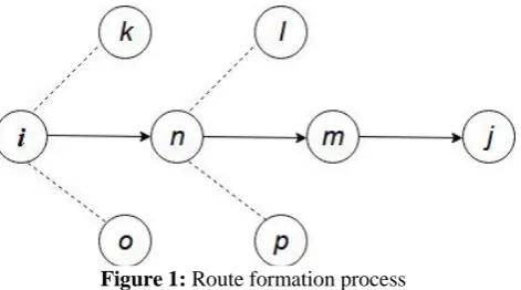
Example 1: As shown in Figure 1, let node i is source node and node j is destination node. Say if node i has data
to send then it looks that neighbor among node k, n and o who is nearer to node j using Haversine formula and GPS locations of respective nodes. Node i finds node o has minimum distance to node j. Now node i calculates the value of minimum transmission power to reach node o and transmit the data packet to node o using calculated value of transmission power. Node o will follow same process and transmit the data packet to node m. The process continuous until data packet reach to node j.
Figure 1: Route formation process
VI. PERFORMANCE METRICS
To measure suitability of proposed technique different packet level metrics are used. Performance metrics used are Energy consumption, End to End Delay and Normalized routing load.
End to End Delay (EED) is average time taken by packets to reach destination in seconds. EED is calculated by taking simulation time difference between transmission (tt) and reception (rt) of packet.
Energy Consumption in terms of energy per bit is calculated using equation (5). Considering current advancement in IC technology, the energy loss within internal circuitry of transmitter and receiver is assumed to be zero.
VII.
RESULT ANALYSIS
Set of simulations are performed for increasing number of nodes with fixed transmission power andconstant speed of nodes. Different sets of nodes are used wise 10, 20, 30, 40, 50, and 100. The simulation time is 100 seconds for each set of parameters listed in table 1.
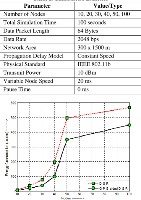
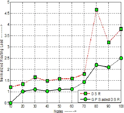
Fig.2 gives comparison of energy consumption. Overall GPS aided DSR performs 30% better than conventional DSR. For nodes less than 30, average of total energy consumption in joule is 41 and 21 and for nodes greater than 30 the values are 420 and 299 for conventional DSR and GPS aided DSR respectively. Results shows energy consumption is decreased by 29% using variable power transmission strategy. From Fig.3 we can compare end to end delay performance of proposed optimization and conventional DSR. It is average time taken by packets to reach destination in seconds and calculated from simulation time difference between transmission and reception of particular packet. The effect of shortest path can be seen fromgraph in the form of E2E delay. Average value for GPS aided DSR is 0.60 ms and for DSR is 0.86ms. Less end to end delay also confirms selection of shortest end to end route. For low node density, large value of end to end delay is because few nodes are available to form the route. Control flooding and route maintenance at local level limits the generation of routing packets. Large number of control packets consumes batterypowerandbandwidthwhichultimatelyreduces routing efficiency. As we can see from Fig. 4, average control packets per data packet transmitted. GPS aided DSR transmits 1.4 control packets per data packet, whereas traditional DSR transmits 11 control packets for 5 data packets. GPS aided DSR avoids global flooding during route discovery process and uses route maintenance at local level. It is to be noted that as number of hopes increases in a route, control packets also increases.
Table 1: Simulation Parameters Parameter Value/Type Number of Nodes 10, 20, 30, 40, 50, 100 Total Simulation Time 100 seconds
Data Packet Length 64 Bytes
Data Rate 2048 bps
Network Area 300 x 1500 m Propagation Delay Model Constant Speed Physical Standard IEEE 802.11b
Transmit Power 10 dBm Variable Node Speed 20 ms
Pause Time 0 ms
Figure 3: End to End Delay (mSec) v/s increasing nodes
Figure 4: Normalized Routing Load v/s increasing nodes
VIII.
CONCLUSION
International organization of Scientific Research
52 | P a g e
REFERENCES
[1]. S. Basagni, I. Chlamtac, and V. R. Syrotiuk, “Dynamic source routing for ad hoc networks using the global positioning system,” in Wireless Communications and Networking Conference, 1999. WCNC. 1999 IEEE, vol. 1. IEEE, 1999, pp. 301–305.
[2]. A. Boukerche, V. Sheetal, and M. Choe, “A route discovery optimization scheme using gps system,” in Simulation Symposium, 2002. Proceedings. 35th Annual. IEEE, 2002, pp. 20–26.
[3]. Y.-B. Ko and N. H. Vaidya, “Location-aided routing (lar) in mobile ad hoc networks,” Wireless networks, vol. 6, no. 4, pp. 307–321, 2000.
[4]. S. Basagni, I. Chlamtac, V. R. Syrotiuk, and B. A. Woodward, “A distance routing effect algorithm for mobility (dream),” in Proceedings of the 4th annual ACM/IEEE international conference on Mobile computing and networking. ACM, 1998, pp. 76–84.
[5]. T. Thongthavorn, W. Narongkhachavana, and S. Prabhavat, “A study on overhead reduction for gps-assisted mobilead-hocnetworks,”inTENCON2014-2014IEEE Region 10 Conference. IEEE, 2014, pp. 1– 5.
[6]. J. Blumenthal, F. Reichenbach, and D. Timmermann, “Minimal transmission power vs. signal strength as distance estimation for localization in wireless sensor networks,” in Sensor and Ad Hoc Communications and Networks, 2006. SECON’06. 2006 3rd Annual IEEE Communications Society on, vol. 3. IEEE, 2006, pp. 761–766.
[7]. V. Rodoplu and T. H. Meng, “Minimum energy mobile wireless networks,” IEEE Journal on selected areas in communications, vol. 17, no. 8, pp. 1333–1344, 1999.
[8]. K. R. Malekshan and W. Zhuang, “Joint scheduling and transmission power control in wireless ad hoc networks,” IEEE Transactions on Wireless Communications, vol. 16, no. 9, pp. 5982–5993, 2017. [9]. Y.-r. Chen, H.-b. Yang, B.-t. Liu, and J.-h. Cheng, “Transmission power optimization algorithm in
wireless ad hoc networks,” in Communications and Mobile Computing (CMC), 2010 International Conference on, vol. 3. IEEE, 2010, pp. 358–363.
[10]. A. O. Ifedayo and M. Dlodlo, “Variable transmission power control in wireless ad-hoc networks,” in AFRICON, 2015. IEEE, 2015, pp. 1–5.
[11]. D. B. Johnson and D. A. Maltz, “Dynamic source routing in ad hoc wireless networks,” in Mobile computing. Springer, 1996, pp. 153–181.
[12]. T. S. Rappaport et al., Wireless communications: principles and practice. prentice hall PTR New Jersey, 1996, vol. 2.
[13]. G. G. de Oliveira Brante, M. T. Kakitani, and R. D. Souza, “Energy efficiency analysis of some cooperative and non-cooperative transmission schemes in wireless sensor networks,” IEEE Transactions on Communications, vol. 59, no. 10, pp. 2671–2677, 2011.
[14]. H. Mahmoud and N. Akkari, “Shortest path calculation: A comparative study for location-based recommender system,” in Computer Applications & Research (WSCAR), 2016 World Symposium on. IEEE, 2016, pp. 1–5.