Prediction of Road Accidents in Semi Supervised Classification Using Map Reducing

ISSN (e): 2250-3021, ISSN (p): 2278-8719

Vol. 09, Issue 6 (June. 2019), ||S (III) || PP 66-76

Prediction of Road Accidents in Semi Supervised Classification

Using Map Reducing

G L Aruna Kumari

1

, Dr T.Jyothirmayi

2

, B.Soujanya

3 1_{Department. of CSE GITAM UNIVERSITY Visakhapatnam, INDIA} 2

Department. of CSE GITAM UNIVERSITY Visakhapatnam, INDIA 3_{Department. of CSE GITAM UNIVERSITY Visakhapatnam, INDIA}

Corresponding Author: G L Aruna Kumari

Abstract:

There is a gigantic need of analysis and predicting the patterns of road accidents across the world in proportion to the increased rate of population and vehicles. In spite of amplified technology, there is a huge gap between the usages of technology to concur the occurrence of road accidents based on similar features. As the big data can be analyzed using map reduce concept with the cloud technologies, the prediction will become more accurate because of large quantity of training set. Here in the proposed work a semi supervised model is developed using Gaussian mixture models to predict the occurrence of accident events which is integrated with Map Reduce(MR) paradigm in BIGDATA. The training data we used has been provided by different government agencies for scientific analysis. Semi supervised analysis and E M algorithm is used on latent data helped to get more accurate results to predict the occurrence of an event with the proposed model. Use of M.R. enhanced the simplicity of working model as the data to be analyzed is in peta bytes and reports should be generated with minimum throughput. The results generated shown more accuracy when proposed model used Gaussian distribution and they are better than other semi supervised models.

Keywords:

E M Algorithm, Bigdata, Map Reduce, Gaussian Mixture Models;

--- --- Date of Submission: 11-06-2019 Date of acceptance: 27-06-2019 --- ---

I.

INTRODUCTION

In developing countries, the issue of road accidents is a major concern. Increasing road traffic/vehicle occupancy could be the reason behind this. There is an increase in accidents over the years. It is very important to regulate traffic on roads to reduce accidents in accident prone zones. Over a decade there is an increase in accidents from 4% to 31% which is an alarming issue. To reduce accidents, it is very important to analyze and identify such road accident patterns.

In 2014, with an average of less than two fatalities per billion vehicle-kilometers, roads in some countries like Switzerland were among the safest in Europe. Yet, there were more than 17000 traffic accidents on Swiss communal roads, cantonal roads and national highways. There were almost 1700 accidents that involved personal injuries on the highway network of approximately 1800 km alone. It is crucial to assess the accident risks as accurately as possible to further reduce this number of accidents. A Gaussian Mixture model is developed using a state of the art methodology to estimate the number of accidents involving personal injury on the Swiss highway network. The developed model not only foresees the number of accidents on a given highway segment but can also be used to find segments that have a high expected number of accidents. While validating, the number of accidents was rightly predicted on 86% of the segments with a tolerance of 25%. Parametric studies can be also conducted using the model, which help in making sure that the risk reduction interventions are effective and efficient. The model can be used by road traffic and road infrastructure engineers and managers during the decision making processes in the planning, construction and maintenance of road networks.

cost for deploying the same on local servers. Hadoop implementation is appropriate for this scenario as we need immediate response to client application.

Factors influencing road accidents:

These can be classified as follows:

1. Vehicle related factors: This includes inherent design limitations or defects due to lack of maintenance, failure of components such as brakes, tires and lighting. Other important factors are visibility, speed and vehicle lighting.

2. Road related factors: Pavement design and conditions, horizontal curves, insufficient lane and shoulder width, vertical curves.

3. Road user related factors: Psychological factors of the users, their alertness and intelligence, drivers‟ patience, experience and age.

4. Environmental factors: Rain, poor visibility, bad weather such as heavy fog, mist and heavy rain also play a crucial role.

II.

LITERATURE ON ROAD ACCIDENTS

A. Neumann and Glenn on (1982) described a theoretical model that relates accident on crest curves to available sight distance. Rather than accident data, this model was developed on intuitively logical relationship and engineering judgment. This model can be used by highway designers to systematically evaluate the cost effectiveness and spot improvement of location with deficient SSD‟s can use the model. The model is as follows:

N= ARH (L)(V) + ARh(Lr)(V)(Far) Where

N = Number of accident on a segment of highways containing a crest curver. ARH = Average accident rate for specific highways

L = Length of highway segment in miles V = Traffic volumes in millions of vehicles. L = Length of restricted sight distance in miles.

Far = A hypothetical accident rate factor that varies based on both the severity of the sight restriction and the nature of the hidden hazard.

Glen on (1983) developed model based on the available literature, according to sufficient evidence it is seen that generally horizontal curves experience higher accident rates than tangents and that accident rates and accidents generally increase as a function of increasing degree of curvature. Glen on horizontal Curve Model reported in the FHWA report accident relationship is presented below:

A= ARs(L)(V)+0.0336(D)(V) Where,

A = total number of accidents on the segment

ARs = accident rate on comparable straight segment in accident L = length of highway segment in miles

V = traffic volume in millions of vehicles D = curvature in degrees

Lc = length of curved component in miles

Zegeer er al (1992) developed the following accident prediction model for the 1991 FHWA study cost-effective improvements for horizontal curves

.

A= [(1.552)(L)(V) + (0.012)(S)(V)](0.978)w) Where

A = number of total accidents on the curve in 3 years period L = length of curves

V = volume of vehicles in million vehicles passing through (both direction) in a 5 Year time. D = degree of curve

S = presence of spiral

W = width of roadway (twice the lane plus shoulder width) on the curve Transportation and Research Laboratory (TRRL) carried out research work in Kenya and

Jamaica and evaluated the combined effect of road elements. The equations developed in this study are as follows:

Y = 1.45 + 1.02X5 + .017X3 (KENYA)

Y = 5.77 + 0.755X1 + 0.275X5 (JAMICA) Where

Y = rate per million vehicle kilometer per year X1 = road width (m)

X2 = vertical curvature (m/Km) X3 = horizontal curvature (degree/Km) X4 = surface irregularity (mm/Km) X5 = junctions per Km

Luis F. Miranda-Moreno et al (2005) developed Alternative Risk Models for Ranking Locations for Safety Improvement. Comparison was made by the authors between performance and practical implications of these models and ranking criteria when they were used for finding dangerous locations. In this research the relative performance of three alternative models is investigated: the traditional binomial model, the heterogeneous negative binomial model and the Poisson lognormal model. The focus in this work, is particularly on the impact of choice of two alternative prior distributions (i.e., gamma versus lognormal) and the effect of allowing variability in the dispersion parameter on the outcome of the analysis.

Fajaruddin Mustakin etal (2008) used multiple regression linear models to study block spot study and accident prediction model. Federal Route (FT50) Batu Pahat - Ayer Hitam was the study area. Following is the regression model

In(APW)0.5=0.0212(AP+0.0007(HTV0.75+GAP1.25)+0.0210(85th PS) Where,

APW= accident point weight age

AP= number of access points per kilometer HTV= hourly traffic volume

Gap= amount of time, between the end of one vehicle and the beginning of the next in second. 85th PS= 85th percentile speed

The model has R-square of 0.9987

As per the results it is seen that existence of a large major junction density, an increase in traffic volume and vehicle speed in federal Route 50 contributed to traffic accident. Influential effect on road traffic accident may be seen by reduced vehicle speed, access point, traffic volume and gap.

Av ascleetal (2010) On this highway, on a stretch of 20km length a camera system has been installed. Traffic data has been recorded since then. Only one accident could be retrieved as the cameras could not capture the traffic completely. Though this data is insufficient to calibrate the model, never the less, the available data is presented here. The reported accidents occurred at 328 km on the highway A1 with cars travelling in the direction. Density and velocity data is presented at a 383 km to the accidents at the side of the accidents 383 km and at kilometer 381 after the accidents referring to condition.

Donatus Iygas, Velmajasiniene etal (2011) analysis of accidents prediction feasibility on the roads of Lithuania. Modeling of road accidents carried out on the basis of 1997-2011. Mathematical models for the optimum selection of road safety improvement measures were constructed using data on fatal and injury accidents on main roads. One of the constructed mathematical model helps in appropriately selecting road safety improvement measures to mathematically decrease the number of people killed under unrestricted amount of trends.

YS = 193.52+0.2t-67.7t1-69.54t2-14.48t3 Where Y= forecasted average value

T= trend variable Ti variable taking the value in the quarter 1 of the year and value 0 in the other quarter. The fourth quarter at the year corresponds to the value of variable.

There is much work done to predict road accident events not sufficient work was done latent variables and also decrease of throughput

III.

DATA PREPROCESSING AND FEATURE COMPUTING

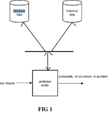
3.1 Data collection and preprocessing

The driver performance data and road structure data, accident based on environmental data. Every thing was collected from the National Informatics Centre(NIC) of road accidents and Data.gov.in. We extracted data on the driver‟s performance during the driving course, the vehicle conditions and also the road features.

We use different features of driving performance recording in the database i.e. throttle, brake, steering wheel, position, speed, acceleration, lane position, distance to same lane vehicle, distance to incoming vehicle. Within each sliding window the statistics of the data are calculated, e.g. minimum, maximum, mean, variance, first-order derivative and etc. Then Expectation Maximization (EM) algorithm for each statistic for safe driving patterns and unsafe driving patterns is used respectively and a Gaussian Mixture Model (GMM) is then estimated.

FIG 1

3.1.1 Feature extraction from driving recording data

The feature f(yi,xi) is computed by comparing the statistical data of each sliding window xi with the

GMM model. A Gaussian function is used to model the system dynamic f(yi-1,yi). we collect the number of past

accidents and violations as a bias for unsafe driving patterns, the road features, traffic features, and atmospheric features etc…as the probability of occurrence of road accident is calculated using The Gaussian probability density function.

3.1.2 The GMM Formulation

The value of a each feature the data in the table of road accidents considered to calculate probability distribution of the feature. As the probability of occurrence of event is calculated based on multiple features The Gaussian mixture model (GMM) is used here as it is a mixture of several Gaussian distributions and can therefore represent different subclasses inside one class. The probability density function is defined as a weighted sum of Gaussians

The Gaussian mixture distribution formula is the form

)

1

(

)

,

|

(

)

(

1

i i s k

i i

s

p

N

x

x

f











Where

(2)

]

)

(

2

1

exp[

2

1

)

,

|

(

_{2 s i} 2

i i

i i

s

x

x

N



















We assume the data is classified into

C

i

i



1,2,...,

k

class that the number of class‟s k is known. The parameters



i

,



i2and

p

i are respect to mean, variance and the probability of a feature belongs to the

3.1.3 The labelled and unlabelled data

The labels of the whole data sequence are needed for training the data bases. Unfortunately, when it comes to our case, labelling all the data sequences is very tedious and expensive. This is for the reason that we can always attach unsafe labels to the data with accidents or violations but it does not hold true for the reverse argument- driving patterns without accidents or violations may be unsafe as unsafe driving patterns do not necessarily lead to accidents or violations. Therefore, we need to manually consider the long driving performance recording and allocate label to every segment. For this, efforts of human annotators with considerable amount of driving experience are needed. Another concern with this labelling scheme is that the data labelling is subjective specifically for a few non-trivial cases and the label from different annotators may be in disagreement with each other.

3.1.4 Semi-supervised learning with Gaussian fields

The use the unlabelled data, we use semi-supervised learning algorithm proposed in [6]. The basis of this approach is Gaussian fields defined on a weighted graph over the labelled and unlabelled data. When it comes to similarity function between observations, the weights of the graph are predefined. Given here is a brief overview of the algorithm:

1. Develop an undirect graph whose nodes correspond to each data point – labelled or unlabelled. 2. Compute the weight of the graph edge from a similarity function, e.g. a Gaussian function.

3. Assign a real-valued function f to each node with the constraint that f equals the label for the labelled data. 4. Minimize the quadratic graph energy function

5. Assign labels to the unlabelled data as per its f function value.

3.1.5 The EM-Algorithm

The expectation maximization (EM) algorithm introduced by Dempster (1977) for maximization likelihood functions with missing data. This algorithm is a popular tool for simplifying difficult maximum likelihood problems. It has two steps; in E-step we compute the expectation and in M-step the maximization of the last step is done and iteration EM-steps continue until convergence occur.

________________________________________________ I. THE EM-ALGORITHM

1. Initialize

θ

(0)

= (

p

₁(0)

,

. . .,p

(0)_k

, m

₁(0)

,

. . .

,m

_k(0)

,D

(0)₁

,

. .. ,D

(0)_k

)

2. (E-step) Compute

P

(r+1)

(

i

|

x

_s

)=

p

i

(r)

N

(

x

_s

|

m

(_ir)

, D

_i(r)

)

∑

i=1 k

p

_i(r)

N

(

x

_s

|

m

_i(r)

, D

_i(r)

)

3. (M-step) Compute

^

m

(_ir+1)

=

∑

s=1 n

P

(r+1)

(

i

|

x

_s

)

x

_s

∑

s=1 n

P

(r+1)

(

i

|

x

_s

)

^

D

_i2(r+1)

=

∑

s=1

n

P

(r+1)

(

i

|

x

_s

)(

x

_s

− ^

m

_i(r+1)

)

2

∑

s=1 n

P

(r+1)

(

i

|

x

_s

)

^

p

(_ir+1)

=

1

n

∑

s=1 n

P

(r+1)

(

i

|

x

_s

)





     





_n s s r n s r i s s r r

x

i

P

m

x

x

i

P

1 ) 1 ( 1 2 ) 1 ( ) 1 ( ) 1 ( 2 i

)

|

(

)

ˆ

)(

|

(

D

ˆ

(

|

)

1

p

ˆ

1 ) 1 ( 1) (r i



 



_

n

s s r

x

i

P

n

4. Iterate steps 2 and 3 until convergence.

IV.

ANALYZING HUGE DATA

As the data is gathered from many origins or various locations and it is huge and it must be processed

with low throughput. And the calculation of mean and variance from the huge origins

μ

i

, σ

i 2

are to be computed by acquiring the data from various sources to overcome the issue of acquiring all data from various sources and giving the common report for the computation of mean for the individual features BIGDATA is used.

4.1 BIGDATA

 Big data is a term that describes the large volume of data – both structured and unstructured – that inundates a business on a day-to-day basis. But it‟s not the amount of data that‟s important. It‟s what organizations do with the data that matters. Big data can be analyzed for insights that lead to better decisions and strategic business moves.

4.1.2 Complexity

 Today's data comes from multiple sources, which makes it difficult to link, match, cleanse and transform data across systems. However, it‟s necessary to connect and correlate relationships, hierarchies and multiple data linkages or your data can quickly spiral out of control.

 The importance of big data doesn‟t revolve around how much data you have, but what you do with it. You can take data from any source and analyze it to find answers that enable 1) cost reductions, 2) time reductions, 3) new product development and optimized offerings, and 4) smart decision making. When you combine big data with high-powered analytics, you can accomplish business-related tasks such as:

 Determining root causes of failures, issues and defects in near-real time.

 Generating coupons at the point of sale based on the customer‟s buying habits.

 Recalculating entire risk portfolios in minutes.

 Detecting fraudulent behavior before it affects your organization.

4.2 Hadoop

Apache Hadoop is an open source software framework for storage and large scale processing of data-sets on clusters of commodity hardware. Hadoop is an Apache top-level project being built and used by a global community of contributors and users. It is licensed under the Apache License 2.0

4.2.1 The Apache Hadoop framework is comprised of the below mentioned modules 1. Hadoop Common: had libraries and utilities required by other Hadoop modules

2. Hadoop Distributed File System (HDFS): a distributed file-system that stores data on the commodity machines, providing very high aggregate bandwidth across the cluster.

3. Hadoop YARN: is a resource management platform that is responsible for managing compute resources in clusters and using for scheduling of users‟ applications.

4. Hadoop MapReduce: a programming model for large scale data processing

MapReduce and HDFS components of Apache Hadoop were originally derived from Google‟s MapReduce and Google File System (GFS) papers respectively.

Apart from HDFS, YARN and MapReduce, the complete Apache Hadoop „platform‟ is now commonly considered to comprise of numerous related projects as well: Apache Pig, Apache Hive, Apache Hbase, and others.

variant respectively. The Hadoop framework itself is mostly written in the Java programming language, with some native code in C and command line utilities written as shell-scripts.

4.3 HDFS and MapReduce

At the core of Apache Hadoop there are two fundamental elements: the Hadoop Distributed File System (HDFS) and the MapReduce parallel processing framework.

4.3.1 Hadoop distributed file system

The Hadoop distributed file system (HDFS) is a distributed, scalable, and portable file-system written in Java for the Hadoop framework. In a Hadoop cluster, each node typically has a single namenode, and HDFS cluster comprises of a cluster of datanodes. This is a typical situation as each node does not need a datanode to be present. Each datanode serves up blocks of data over the network using a block protocol specific to HDFS.

4.4 MAP-REDUCE PARADIGM

Mapreducing, a programming model developed at Google is a sort/merge based distributed computing. Originally it was designed for their in-house search/indexing, however, now it is widely used by more organizations (for instance Yahoo, Amazon.com IBM, etc.). Being a functional style programming (for instance LISP) it can be naturally parallelized across a huge cluster of workstations or PCs. Partitioning of the input data, scheduling the program‟s execution across various machines, managing machine failures and handling the necessary inter-machine communication is taken care of by the underlying system. (This is the basic reason for Hadoop‟s success}.

Mentioned here is the way in which the Map reduce programming works:

 Input is partitioned by the runtime and provided to various Map instances.

 Map (key, value) → (key‟, value‟)

 The run time collects the (key‟, value‟) pairs and allocates them to various Reduce functions so that each Reduce function gets the pairs with the same key‟.

 A single (or zero) output is produced by each Reduce.

 Map and Reduce are user written function

Here too count the mean µ from the given set of datasets map(faeature key, feature value):

// key: feature from data set; value: number of occurances by the feature ; map (k1,v1) à list(k2,v2) for each feature w in value: EmitIntermediate(w, "1");

Mapper

(intermediates)

Mapper

(intermediates)

Mapper

(intermediates)

Mapper

(intermediates)

Reducer Reducer Reducer (intermediates) (intermediates) (intermediates) Partitioner Partitioner Partitioner Partitioner

sh

u

ff

lin

g

Getting Data To The Mapper

 -void map(K1 key,V1 value, OutputCollector<K2, V2> output, Reporter reporter)

 K types implement WritableComparable

 V types implement Writable

V.

PROPOSED SCHEME AND IMPLEMENTATION

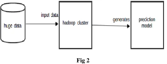
Here in our proposed model the data is analyzed using the GMM in which the latent variable avaluated using the EM algorithm. As the data is huge in volume as it is collected from various sources. To reduce the processing time the calculation of µ of different features is done using the Map Reducing algorithm.

Fig 2

A. Keys and Values:

No value stands on its own in Map Reduce. There is a key associated with every value. Keys recognize related values. Apart from just the values, mapping and reducing receive the (key, value) pairs, The output of each of these functions is identical: both a key and a value should be designated to the subsequent list in the data flow. In GMM the keys are used for the feature values and the values specify the mean µ. The numbers are allocated to weights beginning from input to hidden layer (first hidden layer) weights and ending to hidden layer (last hidden layer) to output layer weights. An easy to use key is provided by the weight no. that is utilized by reducer to obtain all the weight values with identical weight no. to get the overall gradient for that weight no. in the GMM.

B. Chaining of jobs:

Majority of the issues can be resolved through Map-Reduce algorithm and it can be achieved using different mapper and reduced functions. A chaining function is performed, where we take a map function and then reduce function and it builds a chain with various Map-Reduce functions [10]. Map 1 follows Reduce 1, Map 2 follows Reduce 2, Map 3 follows Reduce 3 so on…

Data inputs are usually normalized between a range [0,1] or [-1,1]. We have used a range [-1, 1] for this project. NORMALIZATION FORMULA:-xValue = (xValue / MaxValue).

VI.

RESULTS

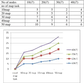
The historical data was taken from 2003 to 2014 which was 10 GB of data to be loaded into HDFS. Although it was a small data set for a hadoop system but the result show significant speed up. We analysed our GMM to calculate the PDF using a Hadoop cluster with 50 worker nodes each containing core i5 Intel processors, 4GB of RAM, and 500 GB of local disk allocated to HDFS. In total, the cluster contains 200 virtual cores. Each node was running Hadoop version 1.0.4 on Ubuntu 12.04 Linux and connected through gigabit Ethernet. We evaluated the speed-up obtained on increasing the number of nodes in the cluster keeping number of map tasks constant and also effect of increasing number of map tasks keeping the number of nodes constant.

We evaluated the speed-up obtained on increasing the number of nodes in the cluster keeping number of map tasks constant and also effect of increasing number of map tasks keeping the number of nodes constant

No of nodes 10(i7) 20(i7) 30(i7) 40(i7) no of map task

10map 5 5 2 4

20 map 5 5 3 5

30 map 7 6 4 5

40map 8 7 5 5

50 map 10 9 6 6

sharply. In cluster with 50 nodes the Hadoop is able to divide map reduce tasks efficiently thus it shows a decrease initially on increasing map tasks and a very slow increase in time on increasing the map tasks further.

Table 2 shows the speedup on increasing the number of nodes in the cluster keeping number of map tasks as constant. The graph of Fig 6 shows a significant speedup on increasing the number of nodes in the cluster. As the number of map tasks is increased the speedup ratio also increases which is clearly depicted from the graph. For 35 map tasks the time on

Increasing the nodes decreases sharply (Light blue line has the highest negative slope). This speed up obtained is linear but with a slope <1.0, this is because of the communication overhead incurred during the map and reduce phase. Increasing the map tasks gives a high speed up ratio due to reduction in the processors idle time through an even distribution of map tasks which is not possible with fewer mapper tasks.

VII.

CONCLUSION

As can be inferred from the tabular and graphical data, the implementation has shown that an Gassiun Mixture model can be parallelize on a Hadoop system using map-reduce technique by exploring the training set parallelism of Gaussian Distributions. The speedup obtained is significant even for a small data set obtained using a cluster of 50 worker nodes. The project has demonstrated a simple programming framework that uses no algorithm optimizations to speed up labeled and unlabelled training by using more and more computer used in a hadoop cluster. The project has also shown that a hadoop system doesn‟t give any significant results with few nodes (1-3) or map tasks (50-100). To achieve the benefit from a hadoop platform it must be scaled to more than 30 nodes cluster.

VIII.

FUTURE SCOPE

large data set. Since the power of hadoop lies in solving problems with huge data sets, in future the results will be taken for TBs of data. The future implementation will also focus on techniques to optimize Map reduce performance for example tuning write no. of map reduce tasks, poor man‟s profiling, writing separate definitions of combiner and partitioner, etc.

REFERENCES

[1]. Neuma and Glenn on (1982),” A Theoretical model that relates accident on crest curves to available sight distance “, Transportation Research Record 923

[2]. Glennon, J., 1985. Effect of Alignment on Highway Safety, Relationship between Safety and Key Highway Features. SAR 6, TRB Ltd., Washington, D.C., pp: 48-63.

[3]. Luis F. Miranda-Moreno, Liping Fu,Frank F. Saccomanno, and Aurelie Labbe 2005 Alternative Risk Models for RankingLocations for Safety Improvement transportation Research Record: Journal of the Transportation Research Board, No. 1908,Transportation Research Board of the National Academies, Washington,D.C,pp. 1–8.

[4]. Fajaruddin Mustakim (2008),“ Black Spot Study and Accident Prediction Model Using Multiplication Linear Regression”.Advancing and intergrating construction education, research and Practice, August 4-5, 2008

[5]. Kushagra Sahu , REVATI PAWAR, SONALI TILEKAR, RESHMA SATPUTE, Stock-exchange forcasting using Hadoop MapReduce technique, International Journal of Advancements in Research & Technology, Volume 2, Issue 04, April 2013.

[6]. Jeffrey and Sanjay Map-Reduce: Simplified processing on large cluster, Google Research Publication 2004.

[7]. BirgulEgeli, MeltemOzturan, BertanBadur, Stock Market Prediction Using Artificial Neutal Networks, Bogazici University, Hisar Kampus,34342,Istanbul, Turkey.

[8]. Mahdi PakdamanNaeini et.al Stock Market Value Prediction Using Neural Networks2010 International Conference on Computer Information Systems and Industrial Management Applications (CISIM) [9]. Cheng-Tao Chu, Sang Kyun Kim,Yi-An Lin, Map-reduce for machine learning on multi core CS.

Department, Standford University 353 Serra Mall, Standford University, Stanford CA 94305-9025. [10]. Jimmy Lin and Michael Schatz Design Patterns for Efficient Graph Algorithms Map Reduce University

of Maryland, College Park,MLG_10 Proceeding of the Eighth Workshop on Mining and Learning with Graph Pages 7885

[11]. The general inefficiency of batch training of gradient descent learning, D. Randall , Volume 16, Issue 10, December 2003, Pages 1429–1451,ACM Digital Library, Elsevier Science Ltd. Oxford, UK, UK [12]. MapReduce Implementation of the Genetic-Based ANN Classifier for Diagnosing Students with

Learning DisabilitiesTung-Kuang Wu1, et.al. 2013.

[13]. Filtering: A Method for Solving Graph Problems in Map reduces, Silvio Lattanzi et.al Google Inc. 2011 ACM 978-1-4503-0743

[14]. Yahoo hadoop Tutorial,

[15]. https://developer .yahoo.com/hadoop/tutorial/

[16]. GSOC proposal to implement neural network, https://issues.apache.org/jira/browse/MAHOUT-364 Zaid Md. Abdul Wahab Sheikh

[17]. Proposal Title: Implement Multi-Layer Perceptrons with backpropagation learning on Hadoop (addresses issue Mahout-342)

[18]. Machine Learning By Andrew Ng. Stanford University COURSERA.ORG Book References [19]. Tom Plunkett-The Oracle Big Data and Hadoop-first edition published by Oracle press

[20]. Neuma and Glenn on (1982),” A Theoretical model that relates accident on crest curves to available sight distance “, Transportation Research Record 923.