Thermodynamic curvature and phase transitions in Kerr-Newman black holes
George Ruppeiner*Division of Natural Sciences, New College of Florida, 5800 Bay Shore Road, Sarasota, Florida 34243-2109, USA (Received 13 February 2008; revised manuscript received 14 May 2008; published 10 July 2008)
Singularities in the thermodynamics of Kerr-Newman black holes are commonly associated with phase transitions. However, such interpretations are complicated by a lack of stability and, more significantly, by a lack of conclusive insight from microscopic models. Here, I focus on the later problem. I use the thermodynamic Riemannian curvature scalarRas a try to get microscopic information from the known thermodynamics. The hope is that this could facilitate matching black hole thermodynamics to known models of statistical mechanics. For the Kerr-Newman black hole, the sign ofRis mostly positive, in contrast to that for ordinary thermodynamic models, whereRis mostly negative. Cases with negativeR include most of the simple critical point models. An exception is the Fermi gas, which has positiveR. I demonstrate several exact correspondences between the two-dimensional Fermi gas and the extremal Kerr-Newman black hole. Away from the extremal case,Rdiverges toþ1along curves of diverging heat capacitiesCJ;andC;Q, but not along the Davies curve of divergingCJ;Q. Finding statistical mechanical models with like behavior might yield additional insight into the microscopic properties of black holes. I also discuss a possible physical interpretation ofjRj.
DOI:10.1103/PhysRevD.78.024016 PACS numbers: 04.70.Dy, 04.60.m, 05.40.a
I. INTRODUCTION
A Kerr-Newman black hole is characterized solely by its mass M, angular momentum J, and charge Q [1]. Such simplicity allows a thermodynamic representation with laws analogous to the standard laws of thermodynamics [2–5]. Previously, I discussed this structure in the context of thermodynamic fluctuation theory [6]. This leads natu-rally to thermodynamic Riemannian geometry; see [7] for a review.
The resulting thermodynamic Riemannian curvature scalar R has been explored by a number of authors for black hole thermodynamics [8–25]. The main contribution of the present paper is an attempt at a physical interpreta-tion of R, and its systematic evaluation for the Kerr-Newman black hole. The analogy with ordinary thermo-dynamics is emphasized, as is the significance of the sign ofR.
The thermodynamic fluctuation formalism requires stability, namely, fluctuations about a maximum in the total entropy. This issue poses difficulty for black holes. In [6] stability was obtained by restricting the number of inde-pendent fluctuating variables. In addition, an infinite ex-tensive environment was employed to have the fluctuations depend only on the known thermodynamics of the black hole.
For an ordinary thermodynamic system,jRjwas inter-preted [26] as proportional to the correlation volume d,
wheredis the system’s spatial dimensionality andis its correlation length. Direct calculations in a number of statistical mechanical models have verified this [7]; see [11] for a more recent review. A thermodynamic quantity,
R, then reveals information normally thought to reside in the microscopic regime,. Thus,Rhas been of interest in black hole physics, which has good thermodynamic struc-tures, but little conclusive microscopic information.
I interpretjRjfor black holes as the average number of correlated Planck areas on the event horizon. Although I give no direct microscopic model evidence, this interpre-tation would seem to be well motivated by the analogy with ordinary thermodynamics.1ZeroRindicates then ‘‘pixels’’ or ‘‘bits’’2on the event horizon fluctuating independently of each other. Diverging jRj, which I take as signalling a phase transition, indicates highly correlated pixels.
R diverges for extremal Kerr-Newman black holes, where the temperature T !0. I demonstrate here, and previously [29], several exact limiting results matching extremal Kerr-Newman black hole thermodynamics to the two-dimensional (2D) Fermi gas (d¼2). Two dimen-sions are consistent with the membrane paradigm of black holes [30].
I also find instances of diverging R where the heat capacitiesCJ;andC;Qdiverge and change sign,
signal-ling a change of stability. Although divergences in these heat capacities were identified by Tranah and Landsberg [31] in 1980, they have been little discussed in the litera-ture. In contrast, I find no diverging R along the Davies curve [4] where the more familiar heat capacity CJ;Q diverges.
1Such an interpretation is consistent with the assumption ‘‘that all the statistical degrees of freedom of a black hole liveon the black hole event horizon’’ [27].
This paper is organized as follows. First, I review the thermodynamic fluctuation picture in [6]. Second, I discuss thermodynamic Riemannian geometry and curvature, in-cluding an attempt at a physical interpretation forR. Third, I calculate R for the Kerr-Newman black hole. Fourth, I compare the results with those in ordinary thermodynamics.
II. THERMODYNAMIC FLUCTUATION THEORY
A major element in my approach is that the black hole resides in an infinite environment, characterized by mass Me, angular momentumJe, and chargeQe. The
thermody-namics of the environment should be extensive; namely, Me,Je, andQe should each scale up in proportion to the
environment’s volume. With this structure, thermodynamic fluctuations require only the known thermodynamics of the black hole. The environment’s thermodynamic properties, which might be difficult to determine (dark matter, etc.), only sets the state about which fluctuations occur.
This structure is thermodynamically unstable if we al-low an exchange of all three variables ðM; J; QÞ [6,31]. Stability requires either a finite environment or a restriction on the number of independent fluctuating variables. In [6] I took the later approach, and considered the stability of seven cases in an infinite environment: fluctuating ðM; J; QÞ, ðJ; QÞ, ðM; QÞ, ðM; JÞ, M, J, and Q.3 Physically, we imagine that one (or two) ofM,J, orQis so slow fluctuating that we can consider it to be essentially fixed.
I use geometrized units withMandQin cm, andJand entropySincm2 [1]. Useful are the Planck length
Lp
ffiffiffiffiffiffiffi
@G c3 s
¼1:6161033 cm; (1)
and the Planck mass
Mp
ffiffiffiffiffi
@c G s
¼2:177105 g; (2)
with@,c, and Gthe usual physical constants. In geome-trized unitsG¼c¼1andLp¼Mp.
The entropy of the Kerr-Newman black hole is [4,33]
SðM; J; QÞ ¼1
8ð2M2Q2þ2
ffiffiffiffiffiffiffiffiffiffiffiffiffiffiffiffiffiffiffiffiffiffiffiffiffiffiffiffiffiffiffiffiffiffiffiffiffi M4J2M2Q2 q
Þ: (3)
To convertSto real units, where it isSbh, use Sbh
kB ¼ 8
L2p
S; (4)
withkBBoltzmann’s constant [6]. The total entropy of the universe is
Stot¼SbhþSe; (5)
where Se is the entropy of the black hole’s environment. The fluctuation probability is given by Einstein’s formula [34],
P/exp
Stot kB
: (6)
Introduce the notation
ðX1; X2; X3Þ ðM; J; QÞ (7)
and
F
@Sbh
@X; (8)
with corresponding properties of the environment denoted by the subscripte. The intensiveFe values are
indepen-dent of the size of the environment.
Let us assume (incorrectly, as it turns out) that the black hole and the environment are fully in equilibrium, with a local maximum forStot. Consider a small fluctuationX
away from this equilibrium. Expanding each of the entro-pies in Eq. (5) to second order yields
Stot¼FXþFeX e þ
1 2
@F @XX
X
þ1 2
@Fe @X
e
X
eXe; (9)
where the coefficients are evaluated at the equilibrium state, which is set by the environment. The conservation laws demand
X¼ X
e; (10)
and a necessary condition for maximum entropy is
F¼Fe: (11)
With a very large environment, the second quadratic term in Eq. (9) is negligible compared with the first. To see this, fix the values ofXe, which equalX. As the
environment is scaled up to infinite size at fixed Fe,Xe
scales up in proportion without limit, and@Fe=@Xe !0.
The ability to drop this second quadratic term is a signifi-cant simplification offered by an infinite, extensive environment.
Equation (9) now can be written as Stot
kB
¼ 1
2gXX; (12)
where the symmetric matrix4
g
8
L2p
@2S
@X@X: (13)
The Gaussian approximation to the fluctuation probabil-ity is
PdX1dX2dXn¼
ffiffiffiffiffiffi jgj p
ð2Þn=2 exp
1
2gXX
dX1dX2dXn; (14)
where jgj is the determinant of g and n¼3 is the
number of independent fluctuating variables. If we set one or two X’s to zero, reducing the value of n,
Eqs. (12) and (14) are only trivially modified. Entropy maximum requires that the matrix g of the remaining
variable(s) be positive definite. Complete discussion of this is given in [6].
The first fluctuation moments are zero [34]:
hXi ¼0: (15)
The second fluctuation moments are
hXXi ¼g; (16)
withg the components of the inverseg
matrix.
Further notation is given in the Appendix, where I define the basic thermodynamic variablesT,, and, the sim-plifying variables , , K, and L, the entropy Hessian determinantsp2,p02, andp002, with numeratorsA,B, andC, and the heat capacities CJ;Q, CJ;, and C;Q. Diverging
heat capacities are important below, and Fig. 1 shows curves of infinities as well as the extremal limiting curve where the temperatureT!0.
III. THERMODYNAMIC RIEMANNIAN GEOMETRY
In this section, I summarize the thermodynamic Riemannian geometry.
A. Thermodynamic metric
The metric follows naturally from the observation that the quadratic form in Eq. (12) transforms as a scalar under any coordinate change becauseStotdepends only on the initial and final thermodynamic states. Hence,
ðlÞ2 ¼ 2Stot kB
¼gXX (17)
is a Riemannian line element. It is unitless and positive definite assuming stability. Its physical interpretation is clear from Eq. (14):the less probable a fluctuation between two states, the further apart they are.
In the definition ofg in Eq. (13),Swas converted to Sbh=kB in real units, essential in Eq. (6). Such a unit
conversion is unnecessary if R is not needed beyond a proportionality constant. However, a quantitative interpre-tation of R in analogy with ordinary thermodynamics requires a unitless line element of the form in the expo-nential of Eq. (14).
To get the metric elements in Eq. (13), I used the special properties of the conserved variables ðM; J; QÞ. Once we have Eq. (13), g transforms as a second rank tensor
under a change of coordinates [7]. Generally, under such a transformation the Hessian form in Eq. (13) will not persist. However, since we know the function S¼ SðM; J; QÞ, there is no need in this paper to change coordinates.
B. Thermodynamic curvature
CalculateRas follows [35]: the Christoffel symbols are
¼12gðg;þg;g;Þ; (18)
where the comma notation indicates partial differentiation. The Riemannian curvature tensor is
R
¼;;þ
; (19)
and the Riemannian curvature scalar is
R¼gR: (20)
R is independent of the choice of coordinate system, suggesting it is a fundamental measure of thermodynamic properties. Since the line element is unitless, R will be unitless.
FIG. 1. Some characteristic curves for the Kerr-Newman black hole; see the Appendix. The curve along which CJ;Qdiverges is the Davies curve. R diverges at the extremal limit and along curves corresponding to a change of stability, which have di-verging CJ;and C;Q.
4In [6], the symbol
For two-dimensional thermodynamic geometries (n¼ 2), all components of the Riemannian curvature tensor may be expressed in terms of the curvature scalarR[35]. Not so in higher dimensions. However, it was argued [36] thatRis the essential quantity in thermodynamic geometry regard-less of the number of independent thermodynamic variables.
For an ordinary pure fluid, a common picture [26] is that of an open subsystem with fixed volumeV surrounded by an infinite environment of the same fluid. The entropy fluctuation is
Stot kB
¼1 2V
1 kB
@2s @x@xx
x; (21)
where s is the entropy per volume (in units of kB per
volume), andx1andx2are the energy and particle number per volume, respectively. The pure fluid line element was written [26] withV omitted:
ðlÞ2 ¼ 1 kB
@2s @x@xx
x; (22)
and has units of inverse volume. The correspondingRhas units of volume.
Logically, however, the pure fluid line element could have been written in the unitless form
ðlÞ2¼ 2Stot kB
¼ 1 kB
@2S @X@XX
X; (23)
with neither the subsystem entropy S nor the conserved energy and particle numberfX1,X2g divided by the con-stantV. The form of this line element matches that of the black hole line element Eq. (17). It has unitlessR.
For the pure fluid, it was noted [26] thatR calculated with the line element Eq. (22) is zero for the pure ideal gas, suggesting that Ris a measure of intermolecular interac-tion strength. Indeed, calculainterac-tions showedjRj to be pro-portional to the correlation volume d for a number of
statistical mechanical models [7,11].
Such calculations dovetailed nicely withRhaving units of volume. However, the units of R are not naturally determined.5 With the equally valid line element in Eq. (23), the fixedV now appears in the denominator of R, andRis unitless. If we imagine the fluid broken up into three-dimensional (d¼3) pieces each of volumeV,jRjis the average number of correlated ‘‘pixels.’’ The physical interpretation ofjRjis then essentially the same regardless of whether or not we pullVout of the line element.
This leads to a possibly useful way to look at black holes. Although there is no fixed subsystem volume to set a scale, the Planck length Lp suggests a physical
constant for this role.6Black hole thermodynamics takes place on the 2D event horizon. It is natural to break it up into square pixels each of area L2p [28]. By analogy with
the pure fluid, I interpret jRj as the average number of correlated pixels. Figure 2 illustrates this physical interpretation.
I cannot presently support this idea with microscopic calculations of a type which were so valuable in ordinary thermodynamics. However, the correspondence in the ex-tremal limit with the 2D Fermi model [29], discussed below, indicates at least consistency with the black hole membrane paradigm [30] which puts all black hole prop-erties on the 2D event horizon.
Note, this interpretation is only of jRj. Janyszek and Mrugała [38] argued that the sign ofR is also important. I amplify on this in Sec. VI.
Finally, in a coordinate system with metric elements of Hessian form, R simplifies. The arguments in [36] allow one to show that with metric elements in Eq. (13),
R¼14ggog ðg
;go; go; g;Þ: (24)
The second derivatives of the metric elements cancel in the calculation.
FIG. 2. The event horizon broken up into Planck area pixels. The dark pixels are portrayed as somehow correlated. I propose that jRjmeasures the average number of correlated pixels.
5My previous arguments about the significance of volume units forR(see, e.g., Sec. VI.B of [7]) may have been overstated. Model calculations and the path integral approach to thermody-namic fluctuation theory [37] are the best way to establishR/ d. However, the pulling out ofVin Eq. (22), and the resulting units of volume forR, is certainly natural and leads to correct results.
C. Background on black hole thermodynamic curva-ture from the entropy metric
A˚ manet al.[16] presented a recent review of thermody-namic curvature in the context of black holes, so my re-marks in this section will be brief. Ferraraet al.[8] were the first to apply thermodynamic curvature to black holes, to calculate critical behavior in moduli spaces. Cai and Cho [9] connected phase transitions in Ban˜ados-Teitelboim-Zanelli (BTZ) black holes to divergingR. They also iden-tified a correspondence with R for the Takahashi gas, suggesting that an appropriate black hole statistical model might be a system of hard rods.
A˚ man, Bengtsson, and Pidokrajt [10] were the first to evaluateRfor various instances of the Kerr-Newman black hole, especially the two-dimensional (n¼2) Kerr and Reissner-Nordstro¨m cases. They also considered a nonzero cosmological constant. Arcioni and Lozano-Tellechea [12] worked out five-dimensional black holes and black rings, including an extensive review. They connected phase tran-sitions to both divergingR and diverging second fluctua-tion moments.
A˚ manet al.[14] examinedRin the context of homoge-neous functions, emphasizing, in particular, cases with R¼0. A˚ man and Pidokrajt [15] investigated Kerr and Reissner-Nordstro¨m black holes in spacetime dimensions higher than four. They found that patterns in four dimen-sions continue to higher dimendimen-sions. Sarkar et al. [17] evaluatedRfor a general class of BTZ black holes, includ-ing quantum corrections to the entropy. Mirza and Zamaninasab [18] worked out the curvature of the full 3D geometry for the Kerr-Newman black hole. They found that R diverges at the extremal limit, but not along the Davies curve. A˚ manet al.[20] reported results on dilaton black holes.
D. Curvature from other than entropy metrics One is certainly not constrained to do thermodynamic Riemannian geometry with fluctuations and its entropy metric. Another possibility is to express the internal energy in terms of its natural variables, M¼MðS; J; QÞ, and construct an energy metric from its Hessian. This was done originally in ordinary thermodynamics by Weinhold [39]. The energy metric is conformally equivalent to the entropy metric [40], with the same angles between vectors, but differentR.
A motivation for exploring other metrics (including the energy metric) is a concern by some authors about the physical validity of cases with R¼0 from the entropy metric. If R is interpreted as a measure of interactions among gravitating particles, one might logically expect jRjto be uniformly large for black holes, where gravita-tional forces are very big.
However, the interpretation of R in this paper takes a different approach. The gravitating particles have presum-ably collapsed to the central singularity, shrinking the
interactions between them to zero volume. The statistics underlying the thermodynamics are envisioned to be on the event horizon. A resultR¼0seems now not so unreason-able. Yet, I present little in the way of microscopic evi-dence for this point of view, so concerns about the physical validity ofR¼0certainly cannot be dismissed.
For the Reissner-Nordstro¨m black hole A˚ manet al.[10] found R¼0with the entropy metric. To avoid this zero curvature, Shen et al. [13] constructed a new entropy metric, replacing QwithandMwithMQ. These authors also argued thatR should signal (by diverging) a phase transition at the Davies curve. Their modified R shows such a divergence. A detailed analogy with the van der Waals phase transition was worked out with their modified metric. The authors also connected to modern themes in particle theory, such as holography and the AdS/ CFT correspondence. Mirza and Zamaninasab [18] evaded zero curvature by evaluatingRfor the full 3D Riemannian geometry. Here,Ris always positive, as will be discussed in Sec. VA. Quevedo and collaborators [19,21,23] sug-gested that this issue requires Legendre invariant metrics to deal with properly. They constructed a detailed framework based on this idea. Medved [24] also gave a recent dis-cussion of these issues.
IV. BACKGROUND ON PHASE TRANSITIONS
Exactly what constitutes a black hole phase transition is somewhat unsettled in the literature. In ordinary thermo-dynamics the modern belief is ‘‘a phase transition occurs when there is a singularity in the free energy or one of its derivatives’’ [41]. Phase transitions can bring about dra-matic contrasts, like between a solid and a gas. Or changes can be more subtle, like the onset of a gradual deformation in crystal structure. Conjectured phase transitions in Kerr-Newman black holes are typically of the more subtle variety, second-order phase transitions associated perhaps with a diverging heat capacity.
Phase transition theory in ordinary thermodynamics typically includes equilibrium between system and envi-ronment. Achieving this with black holes can be difficult. A more serious problem is the lack of conclusive micro-scopic models for black holes. This makes it hard to identify objects as fundamental to phase transition theory as order parameters and correlation functions.
There are then a number of viewpoints of what might be involved in a black hole phase transition: (1) a change in topology, (2) a divergence of a second fluctuation moment, (3) a divergence of a heat capacity, (4) an onset of insta-bility like that in an axisymmetric rotating self-gravitating fluid, (5) a divergence of R, and (6) consistency with the scaling laws of critical phenomena.7
For the Kerr-Newman black hole, there is no topology change except possibly at the extremal limit. Otherwise, the topology is that of the sphere [42].
Second fluctuation moments are connected to quantities such as heat capacities through thermodynamic fluctuation theory [34], so viewpoints (2) and (3) are related, a point not always clear in the black hole literature.
Davies [4] argued that the curve of divergingCJ;Q
con-stitutes a second-order phase transition. However, this has been disputed by a number of authors. One issue is whether or not the Davies curve marks an actual change of stability. I found that it does so only forMfluctuations [6]. Davies [4] also brought up the analogy with the change of sym-metry of an axisymmetric rotating self-gravitating fluid [43]. However, this was questioned [44] since the non-rotating black hole also crosses the Davies curve as charge is increased.
Arguments based on scaling theory usually involve at-tempts to introduce an order parameter. Caiet al.[45] and Kaburaki [46] argued that the extremal limit constitutes a second-order phase transition and proposed the difference between the inner and outer black hole radii as the order parameter. Lousto [47,48] emphasized instead a phase transition along the Davies curve. He used c as
the order parameter, wherecis the angular velocity along
the Davies curve. He also worked out critical exponents and discussed them in the context of scaling theory. Lau [49] also argued that the Davies curve corresponds to a second-order phase transition.
V. KERR-NEWMAN THERMODYNAMIC CURVATURE
In this section, I work outRforðM; J; QÞ,ðJ; QÞ,ðM; QÞ, andðM; JÞfluctuations.M,J, andQfluctuations, withn¼ 1, have R trivially zero, and require no special consideration.8
I go beyond A˚ manet al.[10], and report all situations. In the Kerr-Newman family, these authors focused primarily on Reissner-Nordstro¨m black holes, represented by the geometry of ðM; QÞ fluctuations with J¼0, and Kerr black holes, represented by the geometry ofðM; JÞ fluctua-tions withQ¼0.
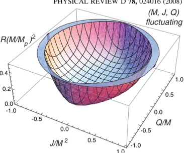
A.ðM; J; QÞfluctuating
Here, allðM; J; QÞfluctuate. By Eq. (17), ðlÞ2 ¼g
11ðMÞ2þ2g12MJþ2g13MQ þg22ðJÞ2þ2g23JQþg33ðQÞ2; (25)
corresponding to a 3D Riemannian geometry (n¼3). This case falls entirely outside the domain of stable fluctuations [6,31], and so I give it only a little attention.
Evaluation with Eq. (20) showsRto be always real and positive, with a minimum of ðMp=2
ffiffiffiffi p
MÞ2 at the origin J¼Q¼0. R is shown in Fig. 3.9 It has no anomalies except at the extremal limit, where it diverges proportional toT1.
Mirza and Zamaninasab [18] also worked out this case. With zero cosmological constant, they found that R di-verges at the extremal limit, but nowhere else. In particular, they found no divergence along the Davies curve. They also found nonzero R for the Reissner-Nordstro¨m case, J¼0. Figure3corroborates these findings.
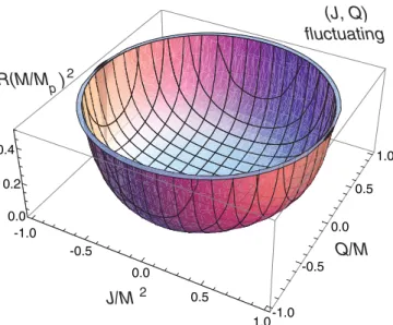
B.ðJ; QÞfluctuating,Mfixed
Here,ðJ; QÞfluctuate at fixedM. By Eq. (17), ðlÞ2 ¼g
22ðJÞ2þ2g23JQþg33ðQÞ2; (26) corresponding to a 2D Riemannian geometry (n¼2). Fluctuations in this case are stable for all states in the physical regime [6].
By Eq. (20), and the definitions in the Appendix,
R¼ðK
5þL2K32K32K2þ3L2K3Kþ2Þ
4KB2 Mp
M 2
: (27)
R is shown in Fig. 4. As is argued in the Appendix,B is J/M 2
-0.5 -1.0
0.0
0.5
1.0
Q/M
-0.5 0.0
0.5 1.0
-1.0
R(M/Mp )2
0.0 0.2 0.4
(M, J, Q) fluctuating
FIG. 3 (color online). RðM=MpÞ2as a function of J=M2and Q=Mfor ðM; J; QÞfluctuations. Ris real, positive, and regular in the physical regime, and diverges as T1at the extremal limit.
8Trivial geometries (n¼1) reflect noninteracting systems. For example, open fluid systems characterized by one fluctuating parameter, usually the internal energy or the temperature, gen-erally do not have interactions, e.g., a gas of photons. With interactions, an additional parameter, like the density, is gener-ally required.
never zero in the physical regime. Hence,Ronly diverges at the extremal limit whereK!0.
Let us examine further the extremal limit. Equations (27), (A6), and (A15) yield the extremal limiting expressions
CJ;Q¼
1
16M3L2T; (28) and
R¼ 2M
2
p
M3L2T: (29)
The limiting product of curvature and heat capacity,
ðRÞ8 L2p
CJ;Q
¼ 2Mp2
M3L2T
8M3L2T 16L2
p
¼1 (30)
is a unitless, scale-free constant independent of where we are on the extremal limiting curve. In Sec. VI B, I evaluate the statistical mechanics of the 2D Fermi gas and demon-strate several exact correspondences with these results at low temperature.
We have from Eq. (16), and the definitions in the Appendix, the dimensionless second fluctuation moments
ffiffiffiffiffiffiffiffiffiffiffiffiffiffiffiffi hðJÞ2i p
@ ¼
1 ffiffiffiffiffiffiffi 2 p
ffiffiffiffiffiffiffiffiffiffiffiffiffiffiffiffiffiffiffiffiffiffiffiffiffiffiffiffiffiffiffiffiffiffiffi K4L2Kþ2K
B
s
M Mp
; (31)
and
ffiffiffiffiffiffiffiffiffiffiffiffiffiffiffiffiffi hðQÞ2i p
e
¼1 2
ffiffiffiffiffiffiffiffiffiffiffiffiffiffi 137:04
s ffiffiffiffiffiffiffiffiffiffiffiffiffiffiffiffiffiffiffiffiffiffiffiffiffiffiffiffiffiffiffiffiffiffiffiffiffiffi 2ðK3þL2KKÞ
B s
; (32)
where e is the electron charge and 137:04¼@=e2 is the fine structure constant. Both fluctuation moments are real
and nondiverging in the entire physical regime. They have maxima of 1=pffiffiffiffiffiffiffi2 and 3.302, respectively, at the origin J¼Q¼0, and decrease to zero as pffiffiffiffiT at the extremal limiting curve.
C.ðM; QÞfluctuating,Jfixed Here,ðM; QÞfluctuate at fixedJ. By Eq. (17),
ðlÞ2 ¼g
11ðMÞ2þ2g13MQþg33ðQÞ2; (33) corresponding to a 2D Riemannian geometry (n¼2). There is a slice of stability [6] in the (pffiffiffiffi, pffiffiffiffi) plane bounded by the extremal limiting curve and the curveC¼ 0, as shown in Fig.5.
By Eq. (20), and the definitions in the Appendix,
R¼ ðL1ÞðLþ1Þ
2KC2 ð3KL64L6þ4K3L48K2L4 6KL4þ36L4þK5L24K4L2þ14K3L2 þ40K2L236KL296L2þ8K5þ4K4
36K332K2þ48Kþ64ÞMp
M 2
: (34)
R is shown in Fig. 6. Despite only a limited slice of stability, located in the ‘‘saddlebags’’ near J=M2 ¼ 1, Ris real everywhere in the physical regime.
Along the lineJ¼0, we clearly haveR¼0, sinceL¼ 1. This was demonstrated by A˚ man et al. [10] who also pointed out that there is no curvature anomaly at the Davies point ðJ=M2; Q=MÞ ¼ ð0;0:8660Þ. I add that no point along the line J¼0lies in the stable slice, as is clear in Fig.5.
Figure6shows a steep drop to negativeRnearQ=M¼ 1. The cut away view shows this as a waterfall shape. Such abrupt behavior, the only case of negative curvature
J/M 2 R(M/Mp )2
Q/M -0.5 -0.5
-1.0
-1.0 0.0
0.0
0.5
0.5
1.0
1.0 0.0
0.2 0.4
(J, Q) fluctuating
FIG. 4 (color online). RðM=MpÞ2as a function of J=M2and Q=Mfor ðJ; QÞfluctuations. Ris real, positive, and regular in the physical regime, and diverges as T1at the extremal limit.
for the Kerr-Newman black hole, reminds one of the abrupt change in sign for the Takahashi gas [50] and for the finite 1D Ising model [51], which will be discussed further in Sec. VI A. None of these negative values fall into the stable slice, however.
Closer to the extremal limit,Rcomes up again, diverg-ing toþ1at all points on the extremal limiting curveK ¼ 0exceptJ¼0. Equations (34) and (A6) yield the extremal limiting expression
R¼ 2M
2
p
M3L2T: (35)
Despite the difference betweenðM; QÞandðJ; QÞ fluctua-tions, this limiting expression is the same as Eq. (29) for ðJ; QÞ fluctuations, and the match to the 2D Fermi gas applies equally well here.
R has an additional divergence, to þ1, at the other boundary of stability, C¼0. R diverges as C2. CJ; diverges asC1, by Eq. (A17).
We have from Eq. (16), and the definitions in the Appendix, the dimensionless second fluctuation moments
ffiffiffiffiffiffiffiffiffiffiffiffiffiffiffiffiffiffi hðMÞ2i p
me ¼
1 ffiffiffiffiffiffiffi 2 p Mp
me
ffiffiffiffiffiffiffiffiffiffiffiffiffiffiffiffiffiffiffiffiffiffiffiffiffiffiffiffiffiffiffiffiffiffiffiK4L2Kþ2K
C s
; (36)
withme the electron mass, and ffiffiffiffiffiffiffiffiffiffiffiffiffiffiffiffiffi
hðQÞ2i p
e
¼1 2
ffiffiffiffiffiffiffiffiffiffiffiffiffiffi 137:04
s ffiffiffiffiffiffiffiffiffiffiffiffiffiffiffiffiffiffiffiffiffiffiffiffiffiffiffiffiffiffiffiffiffiffiffiffiffiffiffiffiffiffiffiffiffiffiffiffiffiffiffiffiffiffiffiffiffiffiffiffiffiffiffiffiffi 4K4þ2L2K38K3þ2L4K
C s
:
(37) Both these quantities are real in the slice of stability. They go to zero aspffiffiffiffiTat the extremal limitK¼0, and diverge
along the curve C¼0. Hence, changing stability is marked by both divergingRand diverging fluctuations.
Note, fluctuations inMexpressed in units of the electron mass are huge. However, in units of the Planck mass they would be much smaller, on the order of the fluctuations inJ andQ.
D.ðM; JÞfluctuating,Qfixed Here,ðM; JÞfluctuate at fixedQ. By Eq. (17),
ðlÞ2 ¼g
11ðMÞ2þ2g12MJþg22ðJÞ2; (38)
corresponding to a 2D Riemannian geometry (n¼2). Stability is confined to a slice bounded by the extremal limiting curve and theA¼0curve, as shown in Fig.7.
By Eq. (20), and the definitions in the Appendix,
R¼ 1
2KA2ðK7þ3K6þ2L2K5þ6L2K45K4 þL4K3þ9L2K39K3þ3L4K2þ4L2K2 8K2þ9L4K21L2Kþ12Kþ9L4
24L2þ16ÞMp
M 2
: (39)
It is shown in Fig. 8. Despite only a limited slice of stability,Ris real and positive everywhere in the physical regime. Its minimum value isðMp=2pffiffiffiffiMÞ2 at the origin. A˚ manet al.[10] computedRforQ¼0, and found it to diverge at the extremal limit. They pointed out that there is no curvature anomaly at the Davies pointðJ=M2; Q=MÞ ¼ ð0:6813;0Þ. This is confirmed by the findings here. I add that no point with Q¼0lies in the stable regime, as is clear in Fig.7.
Rdiverges at the extremal limitK¼0. Equations (39) and (A6) yield the extremal limiting expression
FIG. 7. Stable fluctuation regime for ðM; JÞfluctuating at fixed Qis indicated by þsigns. The case with Q¼0corresponds to the Kerr black hole, which lies entirely out of the stable regime.
Q/M -0.5
-1.0 0.0
0.5 1.0
J/M 2 -0.5 -1.0
0.0
0.5
1.0 R(M/Mp )2
0.0 0.5 1.0
-0.5
(M, Q) fluctuating
R¼ 2M 2
p
M3L2T: (40)
Remarkably, this is the same as Eqs. (29) and (35) found previously.
R has an additional divergence, to þ1, at the other boundary of stability, A¼0. R diverges as A2. C;Q
diverges asA1, by Eq. (A18).
We have from Eq. (16), and the definitions in the Appendix, the dimensionless second fluctuation moments
ffiffiffiffiffiffiffiffiffiffiffiffiffiffiffiffiffiffi hðMÞ2i p
me
¼ 1ffiffiffiffiffiffiffi 2 p Mp
me
ffiffiffiffiffiffiffiffiffiffiffiffiffiffiffiffiffiffiffiffiffiffiffiffiffiffiffiffiffiffiffiffiK3þL2KK
A s
; (41)
and ffiffiffiffiffiffiffiffiffiffiffiffiffiffiffiffi hðJÞ2i p
@ ¼
1 ffiffiffiffiffiffiffi 2 p
ffiffiffiffiffiffiffiffiffiffiffiffiffiffiffiffiffiffiffiffiffiffiffiffiffiffiffiffiffiffiffiffiffiffiffiffiffiffiffiffiffiffiffiffiffiffiffiffiffiffiffiffiffiffiffiffiffiffiffiffiffi 2K4þL2K34K3þL4K
A
s
M Mp
:
(42) Both these quantities are real in the slice of stability. They go to zero aspffiffiffiffiTat the extremal limitK¼0, and diverge along the curveA¼0. Hence, changing stability is marked by both divergingRand diverging fluctuations.
VI. DISCUSSION
In this section, I review evaluations of R in ordinary thermodynamics, and compare with the Kerr-Newman black hole.
A. Curvature in ordinary thermodynamic models
TableIreviews signs and divergences of thermodynamic curvature in several ordinary thermodynamic models. Most table entries are simple models whereRmay be worked out
in closed form. The tendency is negativeRwhere attractive interactions dominate, and positiveR where repulsive in-teractions dominate.10Janyszek and Mrugała [38] empha-sized the importance of the sign of R, and identified the quantum gases, 3D Bose and 3D Fermi, as essential ex-amples with opposite signs.
The signs ofRfor the standard critical point models in TableIare all negative, and have critical point divergences R! 1. This is quite unlike the Kerr-Newman black hole, with its predominantly positive R and divergences R! þ1.
Table I shows a group of weakly interacting systems with ‘‘small’’jRj. Small means on the order of the volume of an intermolecular spacing or less. I view such values of R as physically equivalent to zero, since the meaning of correlation volumes of this size is lost in the ‘‘noise’’ of thermodynamics breaking down as individual atoms and spins become visible. The 1D antiferromagnetic Ising model [52,53] is perhaps misplaced here, since its disalign-ing interactions might propagate a long way. However, for antiferromagnets, the true ordering field is a staggered field, and not the constant field used for the calculations in Table I. A reassessment of this model in these terms might be called for.
There are three cases in TableIhaving both positive and negative curvatures. The 1D q-state Potts model [11,60] has sign related toq. Forq >2, and nonzero field, there are significant regions of negative Rat low temperature. The 2D Potts model has the dimensionality of the Kerr-Newman event horizon. Its Rhas not yet been evaluated, but perhaps its study could yield an appropriate critical line with positiveR.
The Takahashi gas [50] has the typical negativeRin the gaslike phase where attractive interactions dominate, and small jRj in the liquidlike phase where interactions are short range. However, going from one phase to the other by changing the density at constant temperature, there is a pseudophase transition accompanied by a sharp positive
curvature spike. Cai and Cho [9] connected this spike to a phase transition in the BTZ black hole.
An abrupt change in sign ofRis also present in the finite 1D Ising ferromagnet ofN spins [51]. This model has the typical negative R for large N, but a sharp rise to large positive values asNis decreased. Whether or not this result has relevance here is unclear.
Q/M -0.5
-1.0 0.0
0.5 1.0
J/M 2 -0.5
-1.0
0.0
0.5
1.0 R(M/Mp )2
0.0 0.5 1.0
(M,J) fluctuating
FIG. 8 (color online). RðM=MpÞ2as a function of J=M2and Q=Mfor ðM; JÞfluctuations. Ris real and positive everywhere in the physical regime. Rdiverges at both limits of stability.
At the bottom of TableIthere are the 3D Fermi gas [38] and the 3D Fermi paramagnet [61]. Both models have positive R, diverging as T!0. These results lead me now to take a closer look at Fermi gases, particularly the 2D Fermi gas.
B. Curvature for the 2D Fermi gas
For the 3D Fermi gas at lowT,Rseems to diverge [38] asT3=2, and not asT1 in Eq. (29) for the Kerr-Newman
black hole. This motivates me to work out the 2D Fermi gas. By the reasoning leading to Eq. (8.1.3) of [62], the 2D Fermi gas has thermodynamic potential
1
T; T
¼p
T¼kBg
2f
2ðÞ; (43)
with pressurep,expð=kBTÞ, chemical potential , thermal wavelength h= ffiffiffiffiffiffiffiffiffiffiffiffiffiffiffiffiffiffiffi2mkBT
p
, particle mass m, weight factorg ð2sþ1Þ, particle spins, and
flðÞ
1 ðlÞ
Z1
0
xl1dx
1exþ1: (44) I use obvious fluid units for all quantities, includingSand T. The integral in Eq. (44) converges forf2ðÞ, and yields f1ðÞ ¼lnð1þÞ. f0ðÞ andf1ðÞ follow fromf1ðÞ using the recurrence relationfl1ðÞ ¼f0lðÞ[62].
Define the heat capacity at constant particle numberN and constant area Aby
CN;AT
@S @T
N;A
¼NkB
2f2ðÞ f1ðÞ
f1ðÞ f0ðÞ
: (45)
The second equality is by Problem 8.10.ii of [62]. The methods of [62] now yield the limiting lowTexpression
CN;A
AkB ¼
23gmk
BT
3h2 : (46)
EvaluatingRwith Eq. (6.31) of [7] yields
R¼ g12 2f
2ðÞf0ðÞ2þf1ðÞ2f0ðÞ þf1ðÞf1ðÞf2ðÞ ½f1ðÞ22f
0ðÞf2ðÞ2
: (47)
Numerical evaluation over the physical range1< <þ1and0< T <1indicatesRis always positive. The methods of [62] yield the limiting lowT expression:
R¼ 3h
2
23gmk
BT
: (48)
The limitingTdependences ofCN;AandRmatch the corresponding Kerr-Newman black hole quantities [Eqs. (28) and (29)]. This connection to a 2D model is consistent with the membrane paradigm of black holes [30]. Furthermore, the limiting product of curvature and heat capacity,
TABLE I. Thermodynamic curvature for ordinary thermodynamic systems. I give the number of independent thermodynamic parameters n, spatial dimension d, sign of R, and comment on possible divergences. In some systems dis not set, and I denote this with ‘‘ .’’ All signs of Rhave here been put into the sign convention of Weinberg [35]. An indication ‘‘jRjsmall’’ means jRjhas a value on the order of the volume of an intermolecular spacing or less.
System n d Rsign Divergence
3D Bose gas [38] 2 3 T!0
1D Ising ferromagnet [52,53] 2 1 T!0
Critical region [7,26,54] 2 Critical point
Mean-field theory [53] 2 Critical point
van der Waals [7,54] 2 3 Critical point
Ising on Bethe lattice [55] 2 Critical point
Ising on 2D random graph [11,56] 2 2 Critical point
Spherical model [11,57] 2 Critical point
Self-gravitating gas [58] 2 3 Unclear
1D Ising antiferromagnet [52,53] 2 1 jRjsmall
Tonks gas [50] 2 1 jRjsmall
Pure ideal gas [26] 2 3 0 jRjsmall
Ideal paramagnet [52,53] 2 0 jRjsmall
Multicomponent ideal gas [59] >2 3 þ jRjsmall
1D Potts model [11,60] 2 1 þ= T!0
Takahashi gas [50] 2 1 þ= T!0
Finite 1D Ising ferromagnet [51] 2 1 þ= T!0
3D Fermi gas [38] 2 3 þ T!0
R A
CN;A
kB
¼ 3h2 23gmk
BTA
23gmk
BTA
3h2
¼1; (49)
is a unitless, scale-free constant independent of density. The factorAbelowRundoes the traditional pulling out of Ain the ordinary thermodynamic line element.R=Ahere is analogous to R for the Kerr-Newman black hole. The constant products Eqs. (30) and (49) are equal, remarkable for systems apparently so different.
However, note a key difference. The Kerr-Newman black hole entropy Eq. (3) does not go to zero in the extremal limit, as it does for the 2D Fermi gas with its unique ground state. Resolution probably requires a more sophisticated Fermi gas model. Note as well that I have presented no detailed correspondence between the Kerr-Newman black hole thermodynamics and a specific micro-scopic Fermi model. Such a connection is necessary to make the results given here something more than a possi-bly useful direction to explore.
C. Curvature for black hole critical points at nonzeroT
For the phase transitions found at the nonextremal boundaries no appropriate models with evaluated R’s present themselves. The signs of R of the simple critical point models in TableIare all negative, in contrast to the Kerr-Newman black hole results. Hence, I make no attempt here to suggest an order parameter or to evaluate and interpret possible critical exponents and scaling relations between them.
VII. CONCLUSIONS
In conclusion, the following were done in this paper for thermodynamic Riemannian geometry based on the en-tropy metric.
First, I attempted a physical interpretation ofRfor black holes. It was based on analogy with the interpretation in ordinary thermodynamics. Perhaps, this interpretation less-ens concern over the physical plausibility of the occasional resultR¼0.
Second, I reviewed previous evaluations ofRand phase transitions in Kerr-Newman black holes.
Third, I gave a complete evaluation ofR for the Kerr-Newman black hole. In all cases, R was found to be positive in stable fluctuation regimes and to diverge to þ1 at the extremal limit. I also found R to diverge to þ1 at nonzero temperatures along curves of changing stability, where the heat capacitiesCJ;andC;Qdiverge.
Fourth, I argued that the sign of R is important, and tabulated signs in a number of ordinary thermodynamic models. I found that most of the simple critical point models have negativeR. This might make them problem-atic for understanding Kerr-Newman black hole phase transitions. Different models might be required.
Fifth, I noted that the Fermi gas is one of the few known cases in ordinary thermodynamics with large positiveR. I
established several exact correspondences between the 2D Fermi gas and the extremal Kerr-Newman black hole. This suggests that microscopic models with fermions might be useful as a framework for formulating a microscopic de-scription of black holes.
ACKNOWLEDGMENTS
I thank J. A˚ man, B. Andresen, K. Johnston, and H. Quevedo for useful correspondence. I also acknowledge support from the New College of Florida faculty develop-ment fund and help with the figures from Thomas Ruppeiner.
APPENDIX: NOTATION
Notation was defined in [6], and is summarized here. I differ only with the metric elements g, including here the unit conversion factor forSin Eq. (4).
Define the temperature T, the angular velocity , and the electric potentialby [4,31]
1
T
@S @M
J;Q
; (A1)
T
@S
@J
M;Q
; (A2)
and
T
@S
@Q
M;J
: (A3)
Two standard unitless variables are [4]
f; g fJ2=M4; Q2=M2g: (A4)
Simplifying the notation are [31]
fK; Lg fpffiffiffiffiffiffiffiffiffiffiffiffiffiffiffiffiffiffiffiffiffiffiffi1;pffiffiffiffiffiffiffiffiffiffiffiffiffi1þg: (A5)
We may show that 1 T ¼
ðK2þ2KþL2ÞM
4K : (A6)
To be in thephysical regimeof realSandTrequires
þ <1: (A7)
The curve of equality, þ¼1, has K¼T¼0 and constitutes the extremal limit, thought to be unattainable by the third law of black hole thermodynamics [63].
Major components in the discussion of stability are the entropy Hessian determinants:11
11In [6] the metric elementsg
p2 L2
p
8 2
gg1121 gg1222
¼2K33K22L2Kþ2K3L2þ4
16K4M2 ; (A8)
p02 L2
p
8 2
gg2232 gg2333 ¼
K3þL2KKþ1 16M2K4 ; (A9)
and
p002 L2
p
8 2
g11 g13
g31 g33
¼ 1
16K4ðK4þL2K34K3L2K22K2
þL4Kþ2L2K4K2L4þ10L28Þ: (A10)
The numerators ofp2,p02, andp002 are, respectively, A¼ 2K33K22L2Kþ2K3L2þ4; (A11)
B¼K3þL2KKþ1; (A12) and
C¼ ðK4þL2K34K3L2K22K2þL4K þ2L2K4K2L4þ10L28Þ: (A13)
Curves along which these numerators go to zero identify changes of stability accompanied by divergences of heat capacities.A¼0in the physical regime if and only if
¼ð34Þ
2
4ð1Þ2 : (A14)
This curve is shown in Fig. 7. B is never zero in the physical regime, since K0 andL1.C¼0along a single curve in the physical regime, shown in Fig.5, with its algebraic expression too complicated to show here.
Finally, the heat capacities [31]
CJ;QT
@S
@T
J;Q
¼M2KðK2þL2þ2KÞ
4ðL22KÞ ; (A15)
CJ;T
@S
@T
J;
; (A16)
which evaluates to
CJ;¼
M2KðK2þ2KþL2Þ
4C ðL4K2L2þKL2 þ4L2þK3þ4K2þ2K2Þ; (A17)
and12
C;QT
@S @T
;Q
¼M2Kð1þKÞ2ðK2þL2þ2KÞ
4A :
(A18)
CJ;Qdiverges ifL2¼2K. This may be written
2þ6þ4¼3; (A19)
which gives the Davies curve, shown in Fig.1.
[1] C. W. Misner, K. S. Thorne, and J. A. Wheeler,Gravitation (Freeman, San Francisco, 1973).
[2] J. D. Bekenstein, Phys. Rev. D 7, 2333 (1973); 9, 3292 (1974).
[3] S. W. Hawking, Phys. Rev. D13, 191 (1976). [4] P. C. W. Davies, Proc. R. Soc. A353, 499 (1977). [5] P. Hut, Mon. Not. R. Astron. Soc.180, 379 (1977). [6] G. Ruppeiner, Phys. Rev. D75, 024037 (2007).
[7] G. Ruppeiner, Rev. Mod. Phys.67, 605 (1995);68, 313(E) (1996).
[8] S. Ferrara, G. W. Gibbons, and R. Kallosh, Nucl. Phys.
B500, 75 (1997).
[9] R. G. Cai and J. H. Cho, Phys. Rev. D60, 067502 (1999). [10] J. E. A˚ man, I. Bengtsson, and N. Pidokrajt, Gen. Relativ.
Gravit.35, 1733 (2003).
[11] D. A. Johnston, W. Janke, and R. Kenna, Acta Phys. Pol. B
34, 4923 (2003).
[12] G. Arcioni and E. Lozano-Tellechea, Phys. Rev. D 72, 104021 (2005).
[13] J. Shen, R. G. Cai, B. Wang, and R. K. Su, arXiv:0512035v1; Int. J. Mod. Phys. A22, 11 (2007). [14] J. E. A˚ man, I. Bengtsson, and N. Pidokrajt, Gen. Relativ.
Gravit.38, 1305 (2006).
[15] J. E. A˚ man and N. Pidokrajt, Phys. Rev. D 73, 024017 (2006).
[16] J. E. A˚ man, J. Bedford, D. Grumiller, N. Pidokrajt, and J. Ward, J. Phys.: Conf. Ser.66, 012007 (2007).
[17] T. Sarkar, G. Sengupta, and B. N. Tiwari, J. High Energy Phys. 11 (2006) 015.
[18] B. Mirza and M. Zamaninasab, J. High Energy Phys. 6 (2007) 059.
[19] H. Quevedo, Gen. Relativ. Gravit.40, 971 (2008). [20] J. E. A˚ man, N. Pidokrajt, and J. Ward, arXiv:0711.2201v2. [21] H. Quevedo and A. Va´zquez, AIP Conf. Proc.977, 165
(2008).
[22] J. E. A˚ man and N. Pidokrajt, arXiv:0801.0016v1. [23] J. L. A´ lvarez, H. Quevedo, and A. Sa´nchez, Phys. Rev. D
77, 084004 (2008).
[24] A. J. M. Medved, arXiv:0801.3497v2.
[25] Y. S. Myung, Y. W. Kim, and Y. J. Park, Phys. Lett. B663, 342 (2008).
[26] G. Ruppeiner, Phys. Rev. A20, 1608 (1979). [27] M. I. Park, Phys. Lett. B440, 275 (1998). [28] J. D. Bekenstein, Sci. Am.289, No. 2, 58 (2003). [29] G. Ruppeiner, arXiv:0711.4328v1.
[30] K. S. Thorne, R. H. Price, D. A. Macdonald,Black Holes: The Membrane Paradigm (Yale University Press, New Haven, 1986).
[31] D. Tranah and P. T. Landsberg, Collective Phenomena3, 81 (1980).
[32] O. Kaburaki, I. Okamoto, and J. Katz, Phys. Rev. D 47, 2234 (1993).
[33] L. Smarr, Phys. Rev. Lett.30, 71 (1973).
[34] L. D. Landau and E. M. Lifshitz, Statistical Physics (Pergamon, New York, 1977).
[35] S. Weinberg, Gravitation and Cosmology (Wiley, New York, 1972).
[36] G. Ruppeiner, Phys. Rev. E57, 5135 (1998). [37] G. Ruppeiner, Phys. Rev. A27, 1116 (1983).
[38] H. Janyszek and R. Mrugała, J. Phys. A23, 467 (1990). [39] F. Weinhold, Phys. Today29, No. 3, 23 (1976).
[40] P. Salamon, J. Nulton, and E. Ihrig, J. Chem. Phys.80, 436 (1984).
[41] J. M. Yeomans,Statistical Mechanics of Phase Transitions (Clarendon Press, Oxford, 1992).
[42] S. W. Hawking, Commun. Math. Phys.25, 152 (1972). [43] G. Bertin and L. A. Radicati, Astrophys. J. 206, 815
(1976).
[44] L. M. Sokolowski and P. Mazur, J. Phys. A 13, 1113
(1980).
[45] R. G. Cai, R. K. Su, and P. K. N. Yu, Phys. Rev. D48, 3473 (1993).
[46] O. Kaburaki, Phys. Lett. A217, 315 (1996).
[47] C. O. Lousto, Nucl. Phys.410, 155 (1993);449, 433(E) (1995).
[48] C. O. Lousto, Int. J. Mod. Phys. D6, 575 (1997). [49] Y. K. Lau, Phys. Lett. A188, 245 (1994).
[50] G. Ruppeiner and J. Chance, J. Chem. Phys. 92, 3700 (1990).
[51] D. C. Brody and A. Ritz, J. Geom. Phys.47, 207 (2003). [52] G. Ruppeiner, Phys. Rev. A24, 488 (1981).
[53] H. Janyszek and R. Mrugała, Phys. Rev. A 39, 6515 (1989).
[54] D. Brody and N. Rivier, Phys. Rev. E51, 1006 (1995). [55] B. P. Dolan, Proc. R. Soc. A454, 2655 (1998).
[56] W. Janke, D. A. Johnston, and R. P. K. C. Malmini, Phys. Rev. E66, 056119 (2002).
[57] W. Janke, D. A. Johnston, and R. Kenna, Phys. Rev. E67, 046106 (2003).
[58] G. Ruppeiner, Astrophys. J.464, 547 (1996).
[59] G. Ruppeiner and C. Davis, Phys. Rev. A41, 2200 (1990). [60] B. P. Dolan, D. A. Johnston, and R. Kenna, J. Phys. A35,
9025 (2002).
[61] K. Kaviani and A. Dalafi-Rezaie, Phys. Rev. E60, 3520 (1999).
[62] R. K. Pathria, Statistical Mechanics (Butterworth-Heinemann, Oxford, 1996), 2nd ed.