Vol 6, No 1 (2014)

(1)

International Journal of Communication Networks and Information Security (IJCNIS) Vol. 6, No. 1, April 2014

Optimal Spectrum Sensing Threshold for Unequal

Priors Case

Farrukh Javed

1

, Imran Shafi

1

and Asad Mahmood

2

1

Center for Advanced Studies in Engineering Islamabad, Pakistan, 2

School of Computer Science,University of Witwatersrand, Johannesburg, South Africa.

[email protected], [email protected], [email protected]

Abstract: Classical spectrum sensing techniques utilize

maximum likelihood (ML) detection for identification of spectrum holes. The approach is sub-optimal for the case of un-equal priors where the probabilities of channel occupation and vacancy are not the same. Such situations are bound to occur in most commercial bands such as GSM etc and hence are of more interest. The loss in performance has been disregarded as negligible in most of the work done on spectrum sensing techniques. This paper quantifies the effects of changing priors on classical energy detection and infers that the loss in spectrum sensing performance is not negligible. The deterioration is especially considerable at low SNR values and at low probabilities of channel occupation. This paper aims atderiving an optimum threshold for achieving minimum probability of error for unequal prior case. Detection based on the proposed threshold out-performs classical detectors under the assumption that priors are known at the receiver.

Keywords: Cognitive Radios, Spectrum Sensing, ML Detection,

Detection Threshold.

1. Introduction

Rapid expansion in communications has caused an apparent spectrum scarcity whereby, the available spectrum has already been allocated to potential users by various governing agencies. Analysis has revealed that this apparent scarcity is attributable to the inefficient fixed spectrum allocation techniques. This implies that although the spectrum has been licensed to various users but a major portion of this licensed spectrum remains under-utilized. For example, Federal communication commission (FCC) places the spectrum usage in USA between the ranges 15% to 85% at all times [6]. This has opened a new avenue in research to explore more efficient but complex dynamic spectrum access techniques. Dynamic spectrum access envisions the use of licensed spectral bands by smart unlicensed cognitive users that can exploit any opportunities that may exist in the form of temporal or spatial holes. A spectrum hole is that part of the spectrum where the primary users' transmission strength falls below a certain regulated level termed as interference cap by FCC [6]. The smart nodes that form the secondary users are called cognitive radios [7]. A cognitive radio is an evolved software defined radio that in addition to reconfiguration capability also possesses the ability to analyze its surrounding radio environment. This allows the cognitive radio to decide how best to reconfigure itself in existing radio conditions. The capability of a cognitive radio to adapt to its surroundings greatly depends upon the amount and accuracy of information it can acquire about its radio environment. The process by which the cognitive radio

becomes aware of its surroundings is termed as spectrum sensing and is a key challenge for cognitive radios. The prime objective of spectrum sensing is to identify the presence or absence of a licensed (primary) user in a channel. Various spectrum sensing algorithms have been suggested each with its own strengths and weaknesses [1]-[3]. Most of these algorithms utilize some sort of probabilistic modeling to detect the primary user in the observed spectrum [1]. These decision models are generally based on Maximum Likelihood (ML) detection whereby the likelihood probabilities of the signal and noise form the basis of detection [4]. The section II of this paper describes classical ML detection. The section III indicates various performance metrics used in literature to judge the accuracy of the spectrum sensing algorithms [5], [8]. Section IV analyzes classical approaches to decide the threshold level used to discriminate the noise from the signal and their related performance metrics. We have re-derived these metrics in terms of SNR and buffer size to make the comparison more meaningful. An optimal minimum probability of error detector has been suggested in section V. Section VI gives the simulation based results.

2. ML Detection

The ML detection is a binary hypothesis test to confirm the presence or absence of the signal in a buffer size of samples. Assuming that the received signal is being tested for the presence or absence of in white Gaussian noise , the hypotheses would be

. (1)

If | is the likelihood of receiving test statistic for the hypothesis , then it's probability density function would be the weighted sum of two conditional likelihood probabilities | .

| | (2)

(2)

International Journal of Communication Networks and Information Security (IJCNIS) Vol. 6, No. 1, April 2014 amplitude ~ , ! , ~ _", !_" then would

be the sum of squared Gaussian samples and would therefore be Chi - Square distributed with degrees of freedom# . The Chi-Square distribution can be approximated as asymptotically Gaussian | $

%&, !%& in accordance with central limit theorem [12] for a large buffer size . The mean _%_& and variances !_%_& of the two likelihood distributions | can easily be deduced using the definition of variance and the central limiting theorem, however the proof is not given here because of lack of space.

%' " !" (3)

%( ) " !" ! * (4)

!%' 2 2 "!" !", (5)

!%( 2 )2 " !" ! !" ! * (6)

3. Performance Metrics

The various performance metrics used in literature [5] for comparing performance of the spectrum sensing algorithms are summarized below.

3.1 Probability of False Alarm

-

_./

The probability false alarm is a measure of missed opportunities. This is important from a secondary user perspective as it indicates the failure to identify presence of a spectrum hole, while actually it did exist.

01 |

2 3 |

46 | 5

7

8 97 :;<'

=_<' > (7) where Q-Function is the tail probability of the standard normal distribution and is 3 is the sensing threshold. 3.2 Probability of Missed Detection -_?@

The probability of missed detection is a measure of failure to identify an existing primary user in a channel.

01 |

A 3 |

47 | 5

:6

8 9B7 :;<(

=_<( > (8) 3.3 Receiver Operating Curve (ROC)

Receiver operating curve is another conventional method of summarizing the performance of a detector. It is simply a plot of _% versus ₀₁ where _% 1 B _DE is the probability of detection.

% 8 97 :;₌_<(<(> (9) 3.4 Probability of Error -_F

The probability of error is the overall error measure obtained by weighted sum of _DE and ₀₁. The weights

are given according to the prior probabilities of presence of a hole or primary user in the channel.

G | |

8 97 :;<'

=_<' > 8 9B 7 :;_<(

=_<( > (10) 3.5 Sensing Error Floor HIJ

The minimum detection error obtained by choosing a sensing threshold 3_KLM that may result in equal error probabilities of false detection and missed detection is known as sensing error floor NOP .

NOP Q | |

NOP Q 8 97 :;<'

=_<' > 8 9B 7 :;_<(

=_<( > (11)

4. Literature Review

The aim of hypothesis testing is to devise a sensing threshold 3 that suitably divides the two generally overlapping distributions in while optimizing a certain selected performance metrics. For a sensing threshold 3 the ML detection model is

RS T %|U_{T %|U}_'( V W 3 (12)

whereR_S is termed as the likelihood ratio of versus for different values of . W 3 is the ratio of likelihood distributions at sensing threshold 3; W 3

3| / 3| .

4.1 Neyman - Pearson Theorem

An application of Neyman - Pearson theorem [9], [14] – [16], aims at optimizing probability of detection _%under the assumption that a certain fixed level of ₀₁ Z has been assumed as acceptable. The advantage of this approach is that the sensing threshold [-./ can be derived

simply from the noise parameters without any knowledge of primary user transmission. This implies a non-parametric, blind spectrum sensing. The sensing threshold3 _\, _DE and _%in this case can be deduced as

3 \ !%'8: Z %' (13) DE 8 9B7]^₌:;<(

<( > 8 9B=<'

=_<(8: Z B

;_<': ;_<(

=_<( > (14) % 8 9=₌<'

<(8

: _Z;<': ;<(

=_<( > (15)

NOPin this case cannot be defined in this case as ₀₁is fixed while the consolidated probability of error is

G Z 8 9B=₌<'_<(8: Z B ;<(₌:;_<(<'>. (16)

4.2 Sensing Threshold for Achieving HIJ

(3)

3

KLM ;<(=₌<'_;<'=<(

<'_=<( (17)

01, _DE, _G and NOP are all equal in this case and are according to Eqn. (11). _%may be found from either noise or signal parameters.

% 8 9B7`ab₌_<': ;<'> 8 97`ab₌_<(: ;<(> (18) 4.3 Minimum -_FDetector

The minimum P_ddetector is a special case of a more general Bayesian detector which aims at optimizing the Pdassuming that the prior probabilities of hypotheses are known [14]. The likelihood ratio for minimum P_ddetector is given as

We3

\f

g

\ U'

\ U( (19)

and the detection model becomes

| V | . (20)

The sensing threshold 3_\_fcan also be deduced in terms of parameters of likelihood distributions | by considering that e3_\_fh g e3_\_fh g. This results into a quadratic equation that can be simplified to get the sensing threshold as

3

\f

%' %(

!

%(

B !

%'

i9 ;<'_;<(

=_<(j:=_<'j>

;_<'j =_<(j _;_<(j =_<'j _=_<(j =_<'j klem√ K S_ g =_<(j:=_<'j o

( j

(21) wherep / is the ratio of priors. The performance metrics in this case are given by Eqns. (7)– (11)with3 3_\_f, further simplification not being possible. 4.4 Comparison of the Sensing Thresholds

Gis considered here as the most suitable performance metric for comparison. In order to make the comparison more meaningful the _Gcan be reflected in terms of buffer size and N q. Under some reasonable assumptions, G for the three sensing thresholds can be deduced using Eqns. (3) –(6) as

G 7]^ Z

8 r_{√ K S_}: i8: _{Z B s N qtu}₍₂₂₎

G 3KLM 8 v

s]_jK S

_swx(_j K Sj_{_ K S _} y (23) wherez O)| |,*/{O)| | * is a measure of randomness of the signal [4] and varies between 1 to 2. For deducing _Ge3_\_fg in terms of N qand we first convert Eqn. (21) in terms of N qand .

3\f

1 !" 91

2

N q> i!1",91

2

N q> |

| !",}K S ~2 _{K S}• lnep√2N q 1g‚ƒ /

(24)

Ge3\fg 8 v

3\f

!"„2 B … 2 y _1

8 r_{√ K S_}: i 7^f

=‡j„ B s N q 1 tu (25)

The comparison of the analytical results for _G for the three classical sensing thresholds at 0.7 has been displayed in Figure 1. The figure elaborates that for higher

N q and the _Greduces to zero for all three cases. For low N qand the _Gis maximum for 3 _\and3_KLM.

5. Derivation of Optimal Threshold for

Unequal Priors Case

As implied by Eqn. (2) the received test statistic is the sum of two joint distributions ,

, . The minimum _Gdetector described in Eqn. (20) attempts to bifurcate the two distributions by taking their point of intersection as the sensing threshold3_\_f. However as the two distributions acquire distinct parameters; the point of intersection is not an optimal threshold anymore. We propose an optimal sensing threshold for the Bayesian case (with known priors) which aims at minimizing the joint detection error. Assuming a sensing threshold3_ŠT‹, the suggested Maximum Aposterior Probability (MAP) detection model is:

(4)

S \ U_{\ U}(_' T %|U_{T %|U}(_'

V e3

ŠT‹

g

(26) where the posterior ratio threshold would be e3_ŠT‹g

e h3ŠT‹g/ e h3ŠT‹g. It may be noted that Eqn. (26)

reduces to Eqn. (20) for e3_\_fg 1in which case

e h3\fg e h3\fg as used in deduction of Eqn. (21).

In order to achieve simultaneous reduction in the error in detecting joint distributions , , we devise the sensing threshold 3_ŠT‹by equating the error induced in both cases.

46 | 5

7Œ•Ž

47Œ•Ž | 5

:6 p8 97Œ•Ž :;<'

=_<' > 8 9B

7Œ•Ž :;<(

=_<( > (27) As _%₍2 3_ŠT‹2 _%_' we can achieve an approximation of

3ŠT‹ by utilizing the Chernoff bound for Q-function and finding the roots of resulting quadratic equation. The arguments of the Q-function in this case are the Mahlanobi's distances of the distributions from the threshold. The Q-function and its Chernoff approximation

are plotted in Figure 2. The approximation is highly accurate at very low and very high SNRs and quite reasonable otherwise.

3ŠT‹ • %'!_!%(B %(!%'

%(B !%'

=_<(=_<'

=_<(j :=_<'j se %(B %'g ln p e %'!%(B %(!%'g (28) The same equation can be represented in terms of N qand buffer size. For simplicity we represent the repeating term

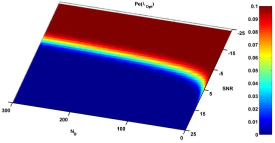
2 N q 0.5 N q z B 1 as ‘́. _Gfor this case is given as Eqn. (30) and has been plotted in Figure 3. Clearly the selected threshold results in extensive improvement in _G reducing the error ceiling considerably.

3ŠT‹• !“” 91 BN q_{‘́ >} | |s 1 _́_•~2 ln p K S_́_• j•t (29)

The threshold can be prevented from becoming complex by keeping a reasonably large buffer size. For example, a buffer size of 400 samples is sufficient to keep the under root terms as positive for SNR ranging from -25 dB to 25 dB and between 0.1 to 0.9.

Ge3ŠT‹g 8 v 3ŠT‹

!"„2 B „2 y

8 r_{√ K S_}: i 7Œ•Ž

=‡j„ B s N q 1 tu (30)

6. Simulation Results

The simulations have been carried out for simple BPSK case considering zero mean AWGN and varying conditions ofN q _%₍/!_%_'. In order to elaborate the effect of priors three different prior ratios p

/ have been simulated assuming

0.3, 0.5 and 0.7. In classical ML case the priors would be equal and p would be unity. However as the prior probability of channel occupation changes in comparison to the probability of channel vacancy , effects of changing priors become prominent. The sum of and remains one in all cases. In Figure4–7 we plot the effects of changing N q on _Gfor three different values of pwhile using the four different sensing thresholds 3 _\, 3_KLM, 3_\G and 3_ŠT‹ for signal detection. Figure 3. Accuracy of Chernoff Approximation

(5)

International Journal of Communication Networks and Information Security (IJCNIS) Vol. 6, No. 1, April 2014 The p is simulated as 1 (classical ML case with equal

priors), 2.33 e 2 g and 0.43e 2 g. The buffer size is fixed at 400. As evident from the results, the changing p has significant bearing on the accuracy of the spectrum sensing algorithm.

Figure 4. Effect of Changing SNR on _G for different p using 3 _\

The effects of changing p for 3 _\are indicated in Figure4. For the typical ML case where the priors are equal, the _DEand ₀₁follow the calculated theoretical results. However as the ratio of priors becomes un-symmetric the results greatly vary from theoretical values because the effects of changing priors have not been considered while selecting the threshold. There is deterioration in _Gfor high because the high prior value for signal distribution and low prior value for noise distribution pushes the distributions closer thus increasing the overlap. This increased overlap results in increased _G. As the two likelihood distributions have been scaled by different factors, the3 _\is not accurate anymore and cannot ensure a fixed ₀₁ as desired. The situation is especially poor where N q and are both very low. This is because the noise distribution which already has a large variance (low SNR) is further shifted to the right overlapping the signal distribution due to multiplication with a large prior value. This results in _DE and ₀₁ both approaching to unity. This amply elaborates that 3 _\ would perform extremely poor in case of low channel occupancy conditions. For high the distributions are pushed further apart than the perceived ML case while calculating the threshold. This results in reduced overlap of the two distributions and improvement in _G.

For3_KLM, the theoretical and simulated results match exactly for equal priors case as reflected in Figure5. However, the change in priors results in variations in _G as the priors were not incorporated while selecting the threshold. _Gdeteriorates for high and improves for low for similar reasons as discussed in the last paragraph. However the _G in this case drops to zero while for the3 _\, it could level off to Z at best. Thus

3KLMoutperforms 3 _\but does not cater for changing priors.

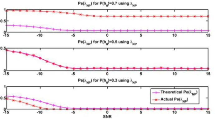
Simulation results reveal that the 3_\Gis the most robust classical detection technique against changing prior values (Figure6). The simulated results are quite similar to the theoretical values for maximum SNR range.

There is improvement for high channel occupancy in comparison to the previous two thresholds. For the low the _Gincreases.

Figure 5. Effect of Changing SNR on _Gfor different p using 3_KLM

As the point of intersection of the two posterior distributions has been considered as the threshold, the asymmetric distributions imply a drop in ₀₁ while on the other hand a sharp increase in _DE. High _DEscaled by a high results in overall increase in _G. This justifies our assumption that the point of intersection of the two posterior distributions is not an optimum threshold for the unequal prior case.

Figure 6. Effect of Changing SNR on _Gfor different p using 3_\G

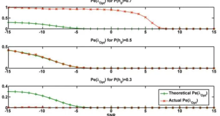
The results for our proposed approach of selecting 3_ŠT‹as the sensing threshold have been displayed in Figure7. The theoretical values of _Gdo not tally with the simulated results except for equal prior case, as these are based on Chernoff approximation. At high , 3_ŠT‹behaves similar to the3_KLMbut as the p approaches to unity, the benefit of using this threshold become obvious. At p

(6)

Figure 7. Effect of Changing SNR on _Gfor different p using 3_ŠT‹

7. Conclusion

The paper aims at quantifying the inadequacies of using classical ML detection for spectrum sensing. The effects of changing prior probabilities of channel occupation or vacancy are simulated and it is concluded that these effects are considerable. The performance degradation is especially aggravated at low SNR values and high variations in prior probabilities. We have also suggested an optimum sensing threshold for minimum _Gwhich is more robust to variations in priors and gives much reduced _Gin comparison to classical sensing thresholds.

References

[1] T. Yucek and H. Arsalan, “A survey of spectrum sensing algorithms for cognitive radio applications,” IEEE Communication Surveys & Tutorials, vol. 11, no. 1, pp. 117-122, firstquarter, 2009.

[2] S. Haykin, “Cognitive radio: Brain-empowered wireless communications,” IEEE J. Selected AreasCommunications, vol. 23, no. 2, pp. 201-220, Feb. 2005.

[3] S. Haykin, “Spectrum sensing for cognitive radio,” Proceedings of the IEEE, vol. 97, no. 5, pp. 849877, May 2009.

[4] H. Tang, “Some physical layer issues of wide-band cognitive radio systems,” IEEE symposium on new frontiers in Dynamic Spectrum Access (IEEE DySPAN 2005), Marylnad USA, pp.151-159, Nov 2005.

[5] Project Coordinator B. MERCIE, “SEnsor Network

for Dynamic and cOgnitive Radio

Access,website(SENDORA),”Report of Project for developing a new approach for Cognitive Radioled by Thales,Eurecom, NTNU, Telenor, KTH, TKK, Universities of Rome, Valencia and Linköping under Contract Number: INFSO-ICT-216076, project website: http://www.sendora.eu/, Jan,2008 – Dec,2010.

[6] B. Benmammar, A. Amraoui, F. Krief, “A Survey on Dynamic Spectrum Access Techniques in Cognitive Radio Networks,” International Journal of Communication Networks and Information Security (IJCNIS) Vol. 5, No. 2, pp. 68-78, August 2013. [7] L. Doyle, “Essentials of cognitive radios,”Book for

Cambridge wireless essentials series,

Cambridgeuniversity press, 1st Edition, pp. 96-105, 2009.

[8] Y. Zeng, Y-L. Liang, A. T. Hoang, and R. Zhang, “A Review on spectrum sensing for cognitive radio: Challenges and solutions,” EURASIP Journal on Advances in Signal ProcessingVolume 2010 (electronic journal), Article ID 381465, 2010.

[9] X. Shi, “Adaptive spectrum sensing for cognitive radios,” Master graduationpaper, publication of the Eindhoven University of technology (TUE). Department of Electrical Engineering, pp. 1-14, 2010. [10]A. J. Coulson, “Blind spectrum sensing using Bayesian sequential testing with dynamic update,”IEEE International Conference on Communications (ICC), Sydney Australia, pp. 1-6, June 2011.

[11]W-Y. Lee, and I. F. Akyildiz, “Optimal spectrum sensing framework for cognitive radio networks,” IEEE trans. on wireless communications, Vol. 7, No. 10, pp 3845-3857, October 2008.

[12]A. D. Polyanin and A. V. Manzhirov, “Handbook of mathematics for engineers and scientists,”Chapman and Hall, pp. 10561-1062, 1st edition,1998.

[13]C. W. Helstrom, “Probability and stochastic processes for engineers,” Macmillan publishing company,pp. 260-266, 2nd edition, 1991.

[14]S. M. Kay, “Fundamentals of Statistical Signal Processing: Detection Theory,” Upper Saddle River, NJ: pp 60-82, 1st Edition, Prentice Hall 1998.

[15]N. Meghanathan, “A Survey on the Communication Protocols and Security in Cognitive Radio Networks,” International Journal of Communication Networks and Information Security (IJCNIS) Vol. 5, No. 1, pp. 19-36, April 2013.