The Effective Use of Student Time: A Stochastic Frontier Production Function Case Study

The Effective Use of Student Time: A Stochastic

Frontier Production Function Case Study

Peter Dolton, Oscar D. Marcenaro and Lucia Navarro

June 2001

Published by

Centre for the Economics of Education

London School of Economics and Political Science Houghton Street

London WC2A 2AE

 Peter Dolton, Oscar D. Marcenaro and Lucia Navarro, submitted February 2001 ISBN 0 7530 1441 6

The Centre for the Economics of Education is an independent research centre funded by the Department of Education and Employment. The view expressed in this work are those of the authors and do not necessarily reflect the views of the Department of Education and Employment. All errors and omissions remain the authors.

Executive Summary

In the economics of education there are relatively few studies which have focused on the mechanism of human capital acquisition. That is, exactly how do people acquire knowledge and what is the relationship between the learning environment and the educational achievement of those receiving the education? The relationship between student study time allocation and examination performance is little understood and is the subject of this research paper.

Education can be regarded as a production process in which a variety of individual study inputs are used to determine a multidimensional output. From the standpoint of the educational institution the way in which resources are used to transform students into well-qualified graduates is of importance. Should individual universities and the taxpayer fund longer and more time intensive courses or are the gains from the extra expenditure worthwhile? From the perspective of the individual student – how best should they allocate their time between formal study in lecture attendance, self-study and leisure and other activities?

The accepted technique for modelling the process of exam performance is the educational production function. This study models the existence of a university production function based on individual student data relating to examination performance. We model the allocation of student time into formal study (lectures and classes) and self study and its relationship to university examination scores using a stochastic frontier production function. The estimation of potential rather than an average educational production function provides an opportunity for estimating the extent of higher education inefficiency. This case study uses unique time budget data and detailed personal records from one university in Spain.

Our econometric results would suggest important policy implications for the university authorities and educational planners. In addition the results may be suggestive for the individual student in their choice of study time and potentially for parents seeking to support their sons and daughters in higher education. Our results suggest:

• Within the formal system of teaching in Spain, both formal study and self study are significant determinants of exam scores but that the former may be up to four times more important than the latter. Hence a student who wishes to maximise their examination score should attend all lectures and classes and minimise their absence from any formal tuition provided by the

university. A logical corollary to this result is that the student should not overindulge in leisure time.

• There is a clear payoff to minimizing the amount of time spent on travel and domestic activities. These results could also have implications for parents who wish to support their student sons and daughters.

• Most obviously for universities the significance of formal study time on performance suggests that they should do all that is in their power to encourage student attendance at lectures and classes or even to make them compulsory university authorities may need to review how many formal contact hours are necessary in each subject. Indeed, if universities operate in a quasi-competitive environment where student performance by university is compared and subsequent employment outcomes are used as performance indicators of universities, they may need to devote more resources to teaching their students.

• University authorities should review the amount of time taken to study for a degree as our results suggest that the academic year could be lengthened and the duration of a degree course shortened if more hours of lectures and classes were presented. Indeed this issue has been on the policy agenda in Spain with the possible shortcoming of degree studies from 5 to 4 years.

• A higher level of student state financial support is most conducive to more favourable exam performance.

• Family income does not seem to matter in the provision of advantage. What does offer an advantage is having provided an educationally privileged background with fewer brothers and sisters (to have to share parental attention).

• Finally, our results provide some support for the view that this ability is not symmetrically distributed among university students and that possibly each student may be constrained by what is possible for someone with their ability. Indeed, controlling for unobserved ability we obtain the result that input of self study time may not matter at all. We also find that self study time may be

The Effective Use of Student Time: A Stochastic

Frontier Production Function Case Study

Peter Dolton, Oscar D. Marcenaro and Lucia Navarro

1. Introduction 1

2. The Student Time Allocation Problem 2

3. Stochastic Frontier Model 6

4. The Malaga University Student Time Survey 9

5. Econometric Results 13

6. Identification, Endogeneity, Instrumental Variables and Ability Bias 22

7. Conclusionsand Policy Implications 31

Appendices 33

Acknowledgements

The authors acknowledge comments on a previous version of this paper presented in Newcastle University.

Peter Dolton is a Professor of Economics at the University of Newcastle. Oscar D. Marcenaro and Lucia Navarro are both at the University of Malaga.

The Centre for the Economics of Education is an independent research centre funded by the Department of Education and Employment. The view expressed in this work are those of the

authors and do not necessarily reflect the views of the Department of Education and Employment. All errors and omissions remain the authors.

1. Introduction

Education is a fundamental contributory factor in the social and economic development of a country. There are a growing number of studies that examine the role which human capital acquisition plays in the economy. Relatively few of them have focused their attention on the mechanism of human capital acquisition. That is, exactly how do people acquire knowledge and what is the relationship between the learning environment and the educational achievement of those receiving the education? Such questions are particularly important given the rapid expansion of all higher education sector in all OECD countries.

From an economic point of view, education can be regarded as a production process in which a variety of individual study inputs are used to determine a multidimensional output, in the form of present and future satisfaction1. From the standpoint of the educational institution the way in which resources are used to transform students into well-qualified graduates is of importance. Should individual universities and the taxpayer fund longer and more time intensive courses or are the gains from the extra expenditure worthwhile? From the perspective of the individual student – how best should they allocate their time between formal study in lecture attendance, self-study and leisure and other activities? Most research which estimates how students achieve their examination grades simply examines the relation between pre-university and university exam scores controlling for personal characteristics and fails to consider how students spend their time in the study process. Indeed there has been a general lack of research on how student time (and its balance) transforms into examination performance. We address this issue in this paper.

Although there have been many studies of educational production the evidence would suggest that we are still a long way from understanding how education is produced in terms of how hours studying is transformed into knowledge. Therefore, there is a rationale for new empirical studies which attempt to shed further light on the process by which these different inputs are transformed into educational outputs.

1

By present satisfaction, we mean the amount of free time which the subject derives from his status as a student. In contrast, future satisfactio ns is a result of the possibility of access to the job market under advantageous circumstances and the social recognition which a high level of attainment affords the student.

The accepted technique for modelling the educational process of exam performance is the educational production function. This study models the existence of a university production function based on individual student data on examination performance. We adopt a production frontier approach, the deviations within which, could be due to errors in specification or measurement or the inefficiency in the process of production. The estimation of potential rather than average educational production functions provides an opportunity for estimating the extent of this higher education inefficiency.

In particular we will investigate the level of inefficiency produced in the transformation of the use students make of their time into educational performance, using the stochastic frontier model. To do this we will use case study data from the higher education system in Spain. This approach is of particular interest if we bear in mind the virtual absence of studies which have followed this line of inquiry.2

The remainder of this paper is organised as follows: in section two we present a simple theoretical model of the students time allocation problem, in section three we set out the stochastic frontier model and the benefits in relation to other possible specifications. In section four we provide a description of the survey of students in one Spanish university. The simple production function econometric results are presented in section five. Section six examines issues of: identification, the endogeneity of pre-university exam scores and unobserved ability bias. Finally, in section seven we discuss possible policy implications and summarise the conclusions.

2. The Student Time Allocation Problem

The seminal paper on the allocation of time by Becker (1965) appeals to the problem of student time allocation in the motivation of his treatment. He then goes on to model time allocation in conjunction with income and the demand for goods which takes us away from the main topic of study in this paper. We are primarily concerned with student time allocation

2

We have found reference to a dated study by Harris (1940) but virtually nothing since then. The exception is Lassibille and Navarro (1986) who present a deterministic model to explain the use which university students make of their time.

between study and leisure (and sleep) and do not consider student earnings and demands for goods3.

Students Preferences over Study Time and Leisure

Assume the student preferences over study time/leisure and exam performance can be represented by the utility function:

U=U(P,L) (1) where P=Performance in Exams

L=Leisure

Assume that exam performance is a sufficient statistic for all future earnings and prospects and hence consumption of goods. Assume uP, uL > 0, and that the utility function is

convex4.

For convenience we will consider leisure to be a sum of two components. The first is the 16 hours of the day over which the individual student is “free” to choose between self study, leisure and sleep. The second is the notional 8 hours per weekday which can be apportioned to formal study in lectures and classes or “stolen” additional leisure. This framework is not a necessary condition for formal analysis but merely an analytical convenience to facilitate diagrammatic analysis.

Time Constraint and Exam Performance

Assume each student can convert time spent on self study, S, and time spent on formal education, F, into examination performance, P, but that this relation is conditional on their, individual specific, innate ability (or intelligence) A.

P=P(F,S,A) (2) where PF > 0, PS > 0 and PA > 0. However we may wish to assume that there is diminishing

returns to study time after some amount of self study and formal education (i.e. PSS<0, PFF<0 )

3

Whilst this is an inevitable simplification, in our data most students do not work in the labour market and hence Becker’s analysis is less directly relevant. In a context where students also have to decide how much time to spend working in the labour market this would not be true.

4

Notice that by assumption in this model students derive disutilit y from extra time spent studying. Our model would therefore be inappropriate for those exceptional students who derive positive utility from extra study hours.

which may also be individual specific. The position may be illustrated for an individual of fixed specific ability A by the Figure 1 below5.

5

We assume for simplicity that the time spent sleeping is constant and equal to eight hours per day.

Optimum F S=0 F0= 8 S0=16 L P P1 F1 Figure 1 F=0 S1, L1

For the individual represented in this figure his/her utility would be maximised by taking L1 leisure which results in S1 time spent on self study, F1 is the time spent on formal education,

and exam performance P1. Notice in this framework (S0 – S1) is the amount of “free” leisure

and sleep time taken and (F0 – F1) is the amount of additional “stolen” leisure taken which is

non-attendance at lectures and classes.

Notice that this simple theory is rich enough to explain the possibility that some individuals who allocate less time to study may end up with higher exam performance, simply due to their higher ability and their more efficient conversion of study time to exam performance. This position is illustrated in Figure 2. For convenience assume formal study time to be fixed and consider only the choice of self study time. This diagram illustrates two individuals, a high ability person, h, and a low ability person, l.

Figure 2

Even with identical study/leisure preferences it is possible with a different self study time to exam performance frontiers indexed by ability, to generate the situation in which the high ability student may study for less time Sh < Sl and still achieve higher exam performance

L P Ll = Sl Lh= Sh S=16 hours Ph Pl S=0 EAl EAh uh ul

Ph > Pl. Of course the position in Figure 2 is only one possibility as, in general, the optimal

choice of L and P depends on the shape of the E transformation and preferences6.

3. Stochastic Frontier Model

As outlined previously, we can compare the behaviour of a student to that of a firm which attempts to obtain an output by the transformation of a set of inputs. In general terms, this process can be represented by the following equation,

y_i = +α X_i'β ε+ _i i = 1, ..., n (3) yibeing a measure of educational performance of individual i, xiis a vector of their explanatory variables,

εi

The idea of this model is that each student’s examination performance is affected by random factors, which are inherently unobservable and distributed normally. These may be associated with assignment to an inspiring teacher, being a member of a good mutual or self help study group, finding the ideal textbook to study from and a whole array of other stochastic factors. The second element which is unobservable in a students potential performance is that their achievement potential is constrained by their inherent (unobservable) ability. This means that each student is limited by how effectively they can “convert” study hours into favourable exam results. The frontier in this context is notionally provided by the students who are most efficient at this conversion. We can effectively measure all other students “inefficiency” or degree of lower ability (as measured relative to the most able students in their cohort). It may be appropriate that the distribution of this unobservable term is asymmetric and we should explicitly model this in a way that allows this to be tested. The stochastic production function facilitates this. The likelihood is that the asymmetry could result from the sorting process of higher education, as it will only admit the top 35% or so, of students from the pre-university exam results distribution (see Appendix A for details of the participation rate in Spain). This means that the selected population who enter university are

6

the selected right tail of the ability distribution7. Figure B1 shows how those who enter university are a selected subsample of the whole potential applicant population. This is the main rationale for the use of the stochastic frontier production function.

If we define yi as the maximum potential performance which students can obtain for any given combination of inputs, the equation (3) can function as an educational frontier production model. This representation requires some assumption concerning the disturbance term. The two hypothesis which appear to satisfy the greatest level of acceptability, lead us to differentiate between the deterministic frontier model and the stochastic frontier model. Both models have in common the parametric nature of their specifications. Doubtless, the first result of considering that any deviation of an observation from the theoretical maximum potential is to be attributed solely to some kind of inefficiency in the educational process of production. From the analytical point of view, this assumes,

y_i = +α X_i'β −u_i i = 1, ..., n (4) ui ≥ 0

where ui represents the inefficiency term8. In contrast, the stochastic frontier production, as outlined by Aigner, Lovell and Schmidt (1977), Meeusen and Van den Broeck (1977) and Battesse and Corra (1977) rely on the premise that the deviations from the production function are due to statistical noise. Such a stochastic factor cannot be attributed to the process of production, and hence should not be embedded in the inefficiency term. The equation (3) representing this final hypothesis is expressed thus9,

y_i = +α X_i'β+ −v_i u_i i = 1, ..., n (5)

ui ≥ 0

A changes.

7

Notice from Figure B1 that this selection process is not a strict truncation as some of these students with low pre-university scores (4.0-6.0) decide to go university and some do not. Formally the stochastic frontier requires a strict truncation, hence the model is only an approximation of the data.

8

Aigner and Chu (1968) suggested two methods for estimating the parameters, assuming that the residuals

uiare positive. These methods are linear programming and quadratic programming. 9

As a result this model can be regarded as a generalisation of the standard regression model, the distinguishing feature of which is the presence of a one s ided error (ui).

where vi is usually assumed to be a normally random variable (distributed independently of ui) with mean zero and variance σ_v2, and ui a non negative error10 typically assumed to be a half-normal distributed variable, with σ_u2> 0. Furthermore, we assume both components of the compound disturbance to be independent and identically distributed (i.i.d) across observations. In this model λ = σ_u2/σ_v2, which is a measure of the degree of asymmetry of the (vi- ui) disturbance term. The larger is λ the more pronounced will be the asymmetry and the correspondingly the OLS estimation is less justified.

Several other specifications can be assumed for the ui inefficiency term, apart from the half normal distribution Aigner, Lovell and Schmidt (1977) and Meeusen and van den Broeck (1977) presented a model which introduced an exponentially distributed disturbance. Later, Stevenson (1980) and Greene (1980) development an alternative specification which used a gamma distribution11. The difficulties of interpreting the latter have led to a greater number of models which use a half normal or exponential specification. It appears that there is no objective criteria for choosing between the two specifications apart from the judgement of the individual researcher. Nevertheless, Battese and Coelli (1988) suggested that the half-normal is the most useful formulation which we could use.

It should be pointed out that there are other methods of analyzing production data, for example Data Envelopment Analysis (DEA)12. Here, for reasons of space, we are not going to examine this method of analysis13. However the motivation for DEA techniques is the same as that which leads us to propose a stochastic frontier model. In contrast to the deterministic approaches of the deterministic frontier and DEA models, the stochastic frontier allows that the variance observed in student performance to be attributed not only to inefficiencies on the educational system but also to incomplete model specification or student heterogeneity. This comparative advantage which the stochastic model has proven to be important when the educational system is analysed, given that the complexity of the factors making up the process of production is such that the factors which can be observed in practice, only make up a small

10

If we were estimating a cost function ui would be a non positive error. 11

See Fried, Lovell and Schmidt (1993) for a broader discussion of this issue. 12

For applications of this technique in the field of education, see Johnes and Johnes (1993), Chalos and Cherian (1995) and Kirjainen and Loikkanen (1998).

13

proportion of the whole. Consequently, whatever deviation there is from the maximum attained performance will contain a strong stochastic component, the identification of which will prove to be crucial when drawing conclusions referred to possible inefficiency sources. There are two additional reasons for not using DEA in our analysis. Firstly, the parametric approach is easier to interpret for firms as institutions. Secondly, we do not need to identify individual observations as inefficient or measure the degree of inefficiency associated with any particular student.

4. The Malaga University Student Time Survey

The data we use to study the student time allocation process is taken from a survey conducted in April 1999 on first and final year students from the different qualifications offered at the University of Malaga. In total, the sample comprises 3722 observations taken from students from forty different subject areas14. In the survey information was collected about personal characteristics, family and school background and academic attributes. Detailed information was requested relating to the amount of time they dedicated to their normal activities. A clear distinction was made between time use on an average weekday and at weekends (details of the questions on time use are reported in Appendix B). The data were collected in the classroom by using a self-completed questionnaire which used individual student identification numbers. This procedure ensured confidentiality and anonymity. The names of each student were not recorded and it was made clear that the survey was not for official university purposes. Hence students were not left with any misunderstanding about the data collection. It was emphasized that the survey was for research purposes only and the data would not be retained or used by the university administration for academic, teaching or assessment purposes. Hence students had no incentive to lie or misreport their responses. Student identification numbers were later used to merge pre-university examination records from central university administrative data.

There is the potential for some bias since the respondents were those who had attended university classes when the survey was carried out, as a result absent students were

14

This sample represents 9.5% all students who matriculated at the University of Malaga during the academic year 1998-1999.

not followed up. Since attendance is around 60% there are a significant minority who do not appear in our sample. This may lead to a higher response rate amongst the more successful students (who usually attend classes more regularly) and the reader should be aware of this when generalizing from the results in this paper. There is also the possibility that sampling only from those attending lectures that we have a sample which is biased in relation to the relative importance of the formal study versus self study balance. If there are a significant number of successful students, not in our sample, who utilise self-study more predominantly in their study schedule then we may understate the importance of self study relative to formal study in the production of exam results. However if absentees are predominantly the worst performing students (which is most likely), then our results may slightly understate the importance of formal study time. All tables show t-statistics alongside the coefficient estimates, to facilitate robustness interpretations of the results.

A major difficulty in any study of time use is to get respondents to accurately remember their time allocation. Juster and Stafford (1991) report that there are many potential biases in asking people to record time use. They suggest that asking respondents to keep a diary is a preferred survey method15.

Unfortunately this was not possible in this study. Juster and Stafford (1991) do however offer some reassurance to this study in an important respect. Namely they suggest that reporting error is minimized when responses involve recording “daily work patterns” with “regular schedules”16. This finding is of most importance if we consider recording information about student study time. All students know how many hours of contact time are involved in their weekly time table, hence to calculate actual contact time they only have to make some adjustment for non-attendance. Likewise the reminder of their weekly schedule will have a regular pattern which may facilitate a reasonable estimate of self study time.

Further support for the validity of our data comes from the construction of the questionnaire which prompts them to be logically consistent in terms of their total hours adding

15

However recent evidence, see Mulligan, Schneider and Wolfe (2000) suggests that time budget studies of this type have biased samples since participating in the survey interferes too much with the lives of the subjects. Hence t his result would support our data collection method.

16

up to these that are available. Around 81% of our respondents record a time budget which adds up to a consistent 24 hours day.

Looking at our average student our data suggests they allocate their weekly time according to the Table 1 below. This allocation is a plausible one. From Table 1 we see that the average person’s time is not quite fully exhausted both on weekdays and weekends. This is a common finding of time budget studies and may be accounted for with other miscellaneous time consuming activities not listed in our questionnaire.

Table 1: Students weekly time allocation (hours)

Weekdays Weekend Formal Education Self Study Private Tuition IT/Language Travel/Domestic Leisure Paid Work Sleep 28.4 15.12 0.95 2.25 8.87 20.46 1.63 38.8 0 4.80 0 0.3 2.0 14.74 0.5 20.84 Total 116.48 43.18

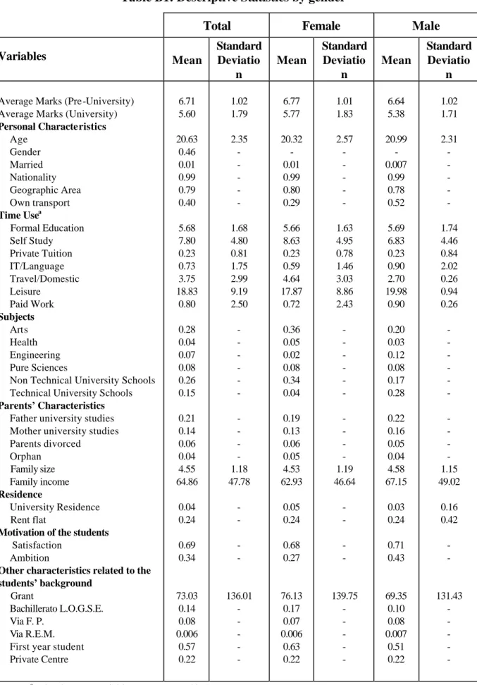
Further biases are possible in the recording of time use. Any measurement error which is systematically related to observed characteristics, e.g. gender, is not a problem as we can condition for this in our estimation. In addition any “pure” measurement error in time recording will also not be a problem since, provided it is random, its influence is captured in the stochastic error term. Of more concern is the possibility of bias generated by a systematic error based on unobservable characteristics. One important example might be that those students who performed badly on their exam might seek some self-justification by underreporting their study time -hence allowing themselves to find an excuse for their poor performance- which did not involve recognising that they may have low ability. It has to be acknowledged that there is very little which can be done about this type of measurement error. In the Appendix B, two tables are presented with the statistics describing the variables used in our estimations. In the first of these the means and standard deviations for the total number of subjects is presented, as well as differences by gender. After deleting observations from the sample which had missing values of one or more of the variables our sample is

reduced to 1976 students. Definitions of the variables are given in the Appendix B. The tables in this appendix indicate that women constitute slightly more than 50% of the sample.

This pattern is specially marked in the areas of Health, Arts and Non Technical University School, as oppose to the Pure Sciences and Engineering (Higher and Technical University Schools) where the proportion is still low17.

When examining the use students make of their time, the first factor to take into account is the time spent attending university classes. The table shows that men, on average, spend the same amount of time attending classes as women each day, but around two hours less in self study. This factor could lead one to think that women put greater effort into their studies, which could be an explanatory factor for their higher performance. This, in quantitative terms, translates into an average grade of almost 0.4 points higher. Something similar happens to the time spent attending IT and language classes. Both, women and men, spend the same amount of time receiving supplementary private tuition, but the latter spend, on average, twenty minutes more acquiring IT and language skills.

The time spent on travel and domestic tasks is higher for women who spend, on average, four hours and forty minutes whereas men spend only two hours and forty. From this we can infer, on the one hand, that women usually participate more in domestic tasks and on the other, that according to our information, 52 % of male students reported to have their own means of transport. In contrast, only 29 % of women responded affirmatively to this question. The latter factor proves to be an important saving in time spent on travel. Finally, it could be interesting to remark that a 43 % of men declared that the principal reason why they decided to study at University was to earn more money by doing an university degree and/or to have more chance of finding a job, but only a 27 % of women declared this as the principal reason.

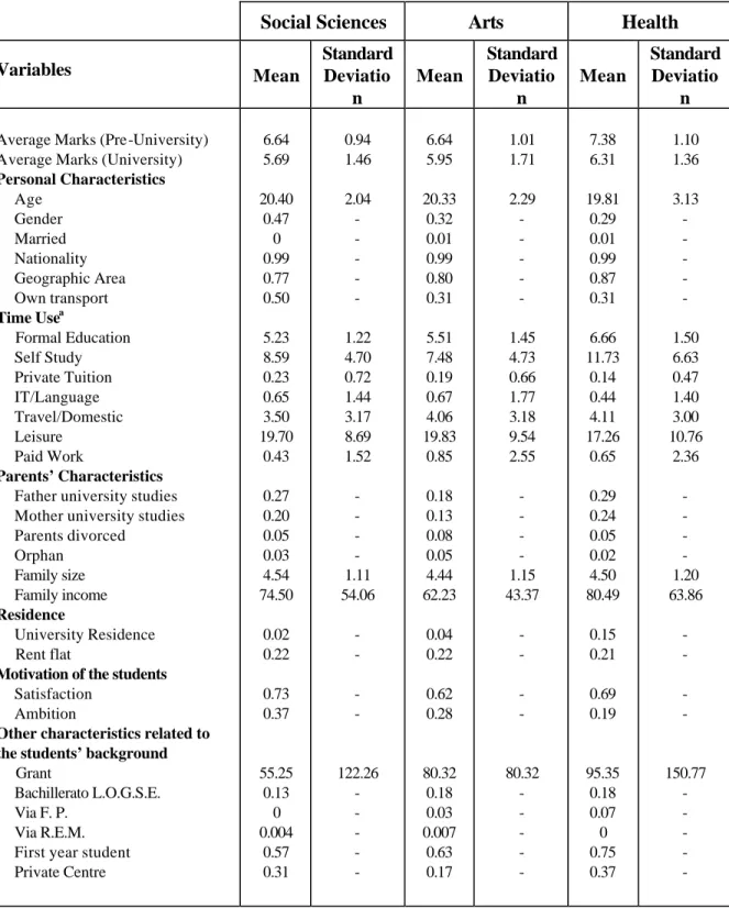
In Table B2 in the Appendix B, a descriptive analysis of the variables is presented, by subject. The main conclusions are presented here. A large difference can be observed in the average performance of students. Thus students of Pure Sciences and Engineering (Higher and Technical University Schools) demonstrate a low average grade, perhaps due to the difficulty of their studies and the high proportion of male students (which could explain that Engineering students are those who spend more time attending private classes). At the other extreme,

Health students are found to have around two points more than the average score, something which could be explained by the rigorous selection process they endure prior to university entrance (as showed by the average university entrance marks) and, equally, to their greater capacity to study. In addition, the variable “number of hours of self study” shows that students of Health, Pure Science and Engineering are the ones who dedicate the most time to their studies. This fact is specially relevant to the first of these subjects with approximately five more hours of study than Non Technical University Schools students (those who spend the least time of their studies). As is logical to assume differences of opposite sign are reflected in the amount of time spent on leisure for both groups of students.

Finally, those who come from “Non Technical University Schools” have the smallest percentage of fathers and mothers who have undertaken university studies, this could be an important explanatory variable in describing the university performance of this type of student.

5. Econometric Results

In this section we discuss the results obtained in the estimation of the stochastic frontier specified in section 2 (equation 5). As we pointed out in the introduction, it is not quite obvious what the outputs of educational process are; i.e. it has a multidimensional output. Bowles (1970) suggests the educational system performs two primary economic functions: socialisation and selection. The first function, socialisation, involves the indoctrination of values and beliefs. The second function, selection, involves the direct effects of schooling on the productivity of the workers18. Unfortunately neither the social nor the economic dimension are directly quantifiable from our data. Our measurement of educational output is based on the average scores obtained by the students during the first semester (academic year 1998-99). These achievement scores must be considered as proxies for productive performance because of the previously outlined unobservable stochastic elements19.

Columns one and two of Table 2 contain the Ordinary Least Squares (OLS) and maximum likelihood (ML) estimates of the educational production function. Column one of that

17

The qualifications which have been includes in each area are detailed in diagram 1 of the appendix A. 18

The relationship between education and productivity has been broadly developed by the “Human Capital Theory” and the “Screening Hypothesis”.

table records the results obtained by OLS and column two presents the ML estimates of the first specification, both use raw (non normalised)20 examination scores (which take no explicit account of subject differences in scores) as dependent variable.

The overall goodness of fit of this model estimated by OLS (as indicated by R2=

0.22) may be considered satisfactory given the difficulty of observing the heterogeneous factors which impact on the educational production process. On the other hand, the result of the likelihood ratio test indicates that the model estimated by ML is significant at standard tolerance levels (for all the specifications).

Estimation by OLS gives unbiased and consistent estimates of all parameters of the frontier function with the exception of the constant term. Hence, we get essentially all the information we would like except the position of the frontier. As a result, the slope coefficients generated by OLS are similar to those obtained by ML. The major difference will be found in the estimation of the intercept term (α), due to the inconsistency of the OLS estimator. The empirical results confirm this theoretical discussion. In fact, the intercept term shows the greatest divergence between both estimates. Hence we will only discuss the coefficients obtained by means of ML estimations in all the specifications.

Examining the variables relating to personal characteristics, age has a positive impact on educational achievement, this may result from the maturity acquired by doing other things before studying or as a consequence of a increased capacity to organise their studies and a better knowledge of the university framework. Alternatively delayed entry to university could have made the student more determined and focused hence more efficient with their time. The result relating to the gender variable is striking. According to the descriptive statistics, women (reference group) attain the highest scores, however the gender coefficient of this variable is insignificant. This could be due (as highlighted in section 3 of this paper) to the fact that this group probably perform better because of the greater time spent studying. In this case it would be the variable “self study” which would explain the higher female students’ output.

19

Some studies of the educational system’s productivity have used achievement test scores as an output measure. Hanushek (1986) has discussed the shortcomings of this measure.

20

Later in this section we normalise university exam scores to control for subject differences in selection and assessment. Here, in Table 2, we simply use raw scores.

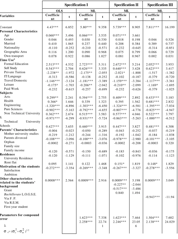
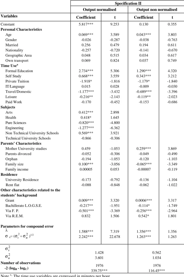
Table 2: Stochastic Educational Production Function (output non normalised)

Specification I Specification II Specification III

OLS ML ML ML Variables Coefficie n t t Coefficie n t t Coefficie n t t Coefficie n t t Constant Personal Characteristics Age Gender Married Nationality Geographic Area Own transport Time Usea Formal Education Self Study Private Tuition IT/Language Travel/Domestic Leisure Paid Work Subjects Arts Health Engineering Pure Sciences

Non Technical University S.

Technical University Schools

Parents’ Characteristics Mother university studies Parents divorced Orphan Family size Family income Residence University Residence Rent flat

Motivation of the students Satisfaction

Ambition

Other characteristics related to the students’ background

Grant

Bachillerato L.O.G.S.E. Via F. P.

Via R.E.M. First year student

Parameters for compound error λ σ ε= (σv 2 +σ_u2)1/2 4.43*** 0.060*** 0.046 0.410 -0.110 0.116 0.078 2.513*** 0.543*** -2.238** -0.313 -1.146*** -0.175* -0.232 0.299** 0.366* -1.320*** -0.902*** 0.362*** -0.971*** 0.427*** -0.004 -0.219 -0.108*** -0.0002 -0.120 -0.120 0.095 -0.272*** 0.0008*** 6.852 3.496 0.493 1.065 -0.252 1.200 0.922 4.532 2.704 -1.972 -0.586 -3.124 -1.703 -0.615 2.241 1.646 -6.896 -5.163 2.674 -6.299 3.655 -0.023 -1.212 -3.096 -0.271 -0.571 -1.129 1.141 -3.354 2.564 5.80*** 0.066*** 0.030 0.237 -0.210 0.090 0.086 2.723*** 0.626*** -2.175** -0.138 -1.181*** -0.206** -0.257 0.394*** 0.339 -1.303*** -0.792*** 0.515*** -0.931*** 0.460*** -0.050 -0.244 -0.100*** -0.0003 -0.150 -0.111 0.122 -0.269*** 0.0009*** 1.623*** 2.258*** 9.358 3.535 0.330 0.440 -0.571 0.968 1.027 5.311 3.335 -2.055 -0.252 -3.389 -2.042 -0.699 2.755 1.323 -6.450 -4.655 3.583 -5.724 3.915 -0.289 -1.316 -3.076 -0.036 -0.689 -1.071 1.468 -3.348 2.916 7.338 22.74 1 5.739*** 0.071*** 0.018 0.208 -0.232 0.075 0.081 2.672*** 0.640*** -2.021* -0.102 -1.159*** -0.210** -0.232 0.409*** 0.395 -1.324*** -0.807*** 0.577*** -0.863*** 0.447*** -0.043 -0.192 -0.978*** -0.0002 -0.183 -0.102 0.151* -0.267*** 0.0009*** -0.227** -0.517*** 0.840 1.623*** 2.246*** 8.905 3.661 0.198 0.384 -0.645 0.799 0.967 5.214 3.428 -1.888 -0.187 -3.384 -2.099 -0.626 2.892 1.562 -6.581 -4.776 4.046 -5.263 3.827 -0.252 -1.042 -2.980 -0.208 -0.843 -0.976 1.819 -3.327 3.198 -2.044 -3.486 1.494 7.464 23.05 6 7.811*** 0.046 0.389 -0.314 0.066 0.002 2.052*** 0.623*** -1.517 -0.379 -1.117*** -1.169* -0.379 0.433*** 0.681*** -1.395*** -0.825*** 0.522*** -1.000*** 0.481*** -0.037 -0.184 -0.101*** -0.0003 -0.036 -0.114 0.148* -0.278*** 0.0009*** -0.943*** 1.504*** 2.138*** 16.199 0.526 0.737 -0.851 0.729 0.031 3.953 3.417 -1.382 -0.720 -3.361 -1.695 -1.025 3.183 2.832 -7.034 -4.947 3.797 -6.512 4.308 -0.219 -1.038 -3.105 0.320 -0.175 -1.123 1.829 -3.556 3.049 -11.94 7.602 24.029

σ_v2 σ_u2 Number of observations R2 F(27,1949 ) -2 (logR - logU) 1976 0.22 17.09*** 1.402 3.695 1976 318.86*** 1.389 3.657 1976 354.90*** 1.401 3.170 1976 235.89***

Note a: The time use variables are expressed in minutes per hour.

Note: * coefficient significantly different from zero at 10% confidence level; ** coefficient significantly different from zero at 5% level; *** coefficient significantly different from zero at 1% level.

Marital status, nationality21 and geographic area are not significant at the standard confidence levels. The indicator variable representing whether a student has their own means of transport has a positive but insignificant coefficient, due possibly to the fact that these students will make important savings in their time spent on travel, and therefore its effect is showed by “travel/domestic” variable.

The second group of explanatory variables measures the use students make of their time. The principle result which deserves attention is that the time spent in formal university study in lectures, seminars, classes and laboratory sessions is positive and highly significant in the determination of student performance. This suggests that there is a direct effect of increased hours spent at the university in formal study. What is less clear in this result is the extent to which this result reflects two different effects: firstly, the higher number of hours provided by the university for the study of a particular subject or secondly the higher rate of attendance by the student at the formal sessions which have been provided for him or her. Unfortunately with our data it is not possible to distinguish between these two separate effects. All we know is the number or hours spent in formal contact time. We do not know how many hours were scheduled for that student.

An equally important result is that self study time is positive and significant as a determinant of performance, but has a much smaller coefficient than the time spent in formal university study. In other words, a student who spends an extra hour at the university in formal study (ceteris paribus) will get better results than those who increase their self study time by one hour.

The most straightforward interpretation of this result is that in terms of producing exam performance, lectures and formal study are up to four times more efficient than self study.

However care should be exercised in the interpretation of this result and its generalizability to other educational institutions, and in particular, to other countries.

Specifically, caution should be expressed since the Spanish higher education system is very structurated and the work required for any course is carefully prescribed during lectures and classes. Course structures are very regulated and little is expected of the students in terms of original research, creative writing or investigate study. Most courses have set textbooks and a prescribed curriculum. A lot of time is spent in lectures and classes, in instruction and practise for the examinations by working through of past examination papers. In such a system we may expect the return to formal study time to be higher than a more flexible system such as that which operates in the UK.

An interpretation of our main result is that each person has a finite capacity to take in subject matter. Hence after a period of intensive self study a person’s capacity for learning new concepts by further time input may be strictly constrained. Hence the efficient allocation of effort may be to study for relatively short periods of time.

A second possible explanation of this result is that opportunity for self study hours is strictly constrained (once one has allowed for formal study time, leisure, travel and sleep). In this interpretation most students only have a limited range of hours to choose to study. In particular in many subjects of study the formal contact hours may be quite high.

On the other hand, it can be seen from Table 2 that time spent in private tuition has a negative effect on students performance. This clearly shows that students who need to attend private tuition are those who are less capable, i.e. with low ability or low motivation, or both. This negative result disappear (in all specifications) when the dummy for first year students is included. The result implies that it is mainly for new, inexperienced students that the private tuition effect is negative. In contrast there is not significant evidence of the influence of time spent learning or improving languages or computer knowledge on students results.

Time spent on travel and domestic tasks, and leisure both have a negative (and significant) influence on scores. The intuition of this result is clear if we think about the student’s available time constraint and that time spent travelling or in domestic activities is not available

21

for study. Therefore he will have to choose among university work (i.e. formal education and study) and other activities.

Time spent working for money has no statistically significant effect. This result is possibly because of the low proportion of students working in the labour market. A possible explanation for this is the low level of university fees in Spain and the level of state grants which obviate the need for students to supplement their income.

Seven dummy variables are used to measure the differential impact on output due to subject differences. The reference group is Social Sciences, so the coefficients measure the effect of each subject relative to this group. From this table one can see that the students who study Health, Arts, and those from Non Technical University Schools attain higher scores than the reference group. In contrast students of Pure Sciences and Engineering (Higher and Technical University Schools) underperform relative to those in Social Sciences. In general these subject variables are highly significant, therefore we can think about the possible existence of large differences across students from different subjects.

Since university selection and entry standards are very different by subject (e.g. Medicine and Engineering -Higher University Schools- are the subjects in most demand and hence entry requirements are highest) it is important to control for this heterogeneity in the determination of performance outcome. One way of doing this is to simply add dummy variables by subject as we have done in Table 2. Alternatively it could be argued that not only are the type of students entering each subject different in ability but also in terms of the marking and assessment schemes. This means that a score of 5.00 in Medicine may mean something totally different to the same score in Arts. To allow for this possibility (and test the robustness of our results on study time for across subject heterogeneity) we normalise our scores within subject. Hence we measure each person’s performance relative to the mean score of their subject peers. In this way we aim to control for ability differences by subject of the students, and the possible heterogeneity of assessment methods by subject.

In the normalised22 results we would expect that the variance of the dependent variable would be substantially reduced and hence the R2 of OLS on the scope for the regressors to

22 n i Scores Normalised subject subject i Deviation dard S Scores Average Scores ,.., 1 ; tan = = −

explain this dependent variable would be considerable reduced. This is confirmed in Table 3. All the coefficients in this table are of the same sign as those tabulated in Table 2 but are smaller (in absolute terms) as a result of the origin and scale change.

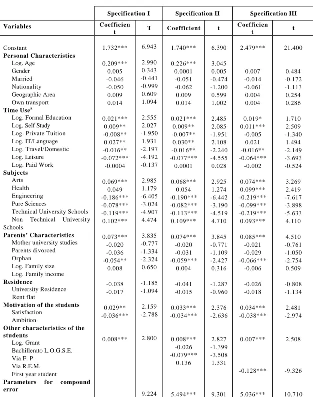
Table 3: Stochastic Educational Production Function (output normalised)

Specification I Specification II Specification III

OLS ML ML ML Variables Coefficie n t T Coefficie n t t Coefficie n t t Coefficie n t t

Constant Personal Characteristics Age Gender Married Nationality Geographic Area Own transport Time Usea Formal Education Self Study Private Tuition IT/Language Travel/Domestic Leisure Paid Work Parents’ Characteristics Mother university stud. Parents divorced Orphan Family size Family income Residence University Residence Rent flat Motivation of the student Satisfaction Ambition Other characteristics of the students Grant Bachillerato L.O.G.S.E. Via F. P. Via R.E.M. First year student

Parameters for compound error λ σε= (σv 2 +σ_u2)1/2 -0.684* 0.039*** -0.0004 0.251 -0.082 0.068 0.042 1.196*** 0.286*** -1.312** -0.181 -0.668*** -0.098* -0.216 0.241*** -0.249 -0.132 -0.067*** -0.0001 -0.117 -0.078 0.058 -0.140*** 0.0005*** -1.857 3.809 -0.009 1.116 -0.320 1.203 0.857 3.765 2.498 -1.983 -0.588 -3.119 -1.644 -0.980 3.530 -0..253 -1.248 -3.288 -0.281 -0.961 -1.261 1.196 -2.960 2.638 0.122 0.041*** -0.009 0.176 -0.122 0.056 0.045 1.275*** 0.329*** -1.319** -0.107 -0.697*** -0.112** -0.204 0.261*** -0.045 -0.145 -0.065*** -0.0001 -0.128 -0.074 0.069 -0.143*** 0.0005*** 1.403*** 1.276*** 0.338 3.772 -0.198 0.551 -0.563 1.021 0.919 4.303 3.075 -2.051 -0.340 -3.391 -1.919 -0.939 3.893 -0.441 -1.314 -3.370 -0.177 -1.043 -1.216 1.410 -3.016 2.970 6.277 19.913 0.096 0.044*** -0.017 0.169 -0.131 0.048 0.043 1.247*** 0.328*** -1.245** -0.071 -0.682*** -0.115** -0.184 0.252*** -0.044 -0.120 -0.064*** -0.0002 -0.145 -0.070 0.082* -0.141*** 0.0006*** -0.119* -0.262*** 0.548* 1.397*** 1.269*** 0.254 3.891 -0.354 0.525 -0.611 0.867 0.875 4.195 3.074 -1.920 -0.226 -3.362 -1.971 -0.839 3.765 -0.440 -1.107 -3.284 -0.364 -1.185 -1.151 1.689 -2.988 3.226 -1.818 -3.044 1.800 6.325 20.040 1.341*** -0.026 0.287 -0.185 0.048 -0.004 0.919*** 0.333*** -1.015 -0.262 -0.675*** -0.086 -0.256 0.270*** -0.042 -0.112 -0.066*** 0.0001 -0.058 -0.082 0.073 -0.151*** 0.0005*** -0.536*** 1.283*** 1.207*** 4.699 -0.529 0.953 -0.842 0.887 -0.080 3.082 3.206 -1.533 -0.877 -3.436 -1.472 -1.173 4.211 -0.426 -1.073 -3.436 0.241 -0.503 -1.385 1.545 -3.279 3.247 -11.66 6.278 20.60 6 σ_v2 σ_u2 Number of observations R2 F(27, 1949) -2 (logR - logU) 1976 0.04 4.51*** 0.549 1.080 1976 111.92*** 0.546 1.065 1976 128.83*** 0.550 0.906 1976 240.38***

Note a: The time use variables are expressed in minutes per hour.

Note: * coefficient significantly different from zero at 10% confidence level; ** coefficient significantly different from zero at 5% level; *** coefficient significantly different from zero at 1% level.

Unsurprisingly, the family income variable is not significant, since family income may be expected to affect the demand of higher education but not necessarily the students performance at this educational level. We also include dummy variables related to the type of accommodation, but these have no influence on scores.

Two variables which merit attention are those relating to the motivations of students23. According to the first such variable, “satisfaction”, those students who did not get into the course they wanted to at university do not perform significantly worse than those who did. In contrast, if the principal reason why they decided to study at University was to earn more money and/or to have a better chance of finding a job, then their academic performance falls.

The remaining variables considered in our estimation pick up some other characteristics related to the students’ educational background. The coefficients of these variables indicate: firstly, there is a clear positive correlation between the amount of state financial support received by the grant holders and their academic results24. This suggests that funds devoted to grants may be used as an important tool from the educational policy point of view. Secondly, the students who continued to higher education from Bachillerato

L.O.G.S.E.. seem to perform worse as compared to those coming from B.U.P. (Secondary

School in the old educational system). This means that the changes introduced by the reform of the educational system (at the Secondary School level) do not contribute to improved student performance. Nevertheless, this result must be treated with caution, because the reform of the educational system (L.O.G.S.E, 1990) had only just been introduced and only affected the first year students in our survey25. As pointed out in Appendix A the vocational track is for the less academic students, thus the negative sign found in the estimations for the variable “Via F.P.” is not unexpected.

The last variable included in Tables 2 and 3 is a dummy variable, which enables us to distinguish between the differential impact on educational achievement of first year students as

23

As can be seen from Table C1 (Appendix C), the results of our estimations do not change in a significant way when motivation variables are dropped.

24

The level of the state support grant is “means-tested” on family income but is in addition payable only to those students with a specified minimum level of exam performance. In our data this variable is correlated with family income but uncorrelated with pre-university exam performance.

25

This is the reason why the variables “Via Bachillerato LOGSE” and “First year students” are included in different specifications.

compared to final year students26. The negative sign of this variable may be a consequence of the lower capacity of first year students to organise their studies and an inferior knowledge of the university framework compared to final year students. Alternatively, in the first year of higher education students may be deliberately taking more leisure time in order to make friends and appreciate the university experience since they are aware that the burden or getting a job and the importance of exam performance will become relatively much more important in their later years of university study.

The robustness of our results has been tested in several different ways. As reported in Table C2 (Appendix C), when a Cobb-Douglas functional form27 is used (instead of a linear functional form) to examine the sign and significance level of the variables considered in the different specifications. Basically these remain the same as in Tables 2, 3. Hence, Table C2 provides additional evidence about the stability of the coefficients found.

Finally, is interesting to examine the variance decomposition provided by estimates of the stochastic frontier, since it allows for both noise and inefficiency. The variance of the composite error (ε) is not _σε2_=σ

v2+σu2. As Greene (1993) points out Var(u)=_π−2_σ

2 2

u, due

to the asymmetry of the disturbance term. Hence the contribution of the variance of u to the total variance is,

2 2 2 2 2 2 2 ) ( ) ( v u u Var u Var σ σ π σ π ε ₊       −       − =

as a consequence, approximately 50 percent28 of the variance of the composite error is caused by educational process inefficiency, while the remaining 50 percent represents unexplained variability. A possible interpretation of this result is that a portion of the unexplained variance in estimated educational production function may be due to time use inefficiencies by students.

26

The variable “age” is not included in Specification III because of the high correlation with the variable “first year students”.

27

Additional estimation was undertaken using a transcendental logarithmic functional form (translog). However our model includes too many independent variables to find a stable set of coefficients for the interaction effects of the variables.

28

This figure does not vary much among the specifications reported (53 % in specifications I and II, and 49% in specification III).

Another possible instrument to measure the relative weight of the inefficiency in our estimations is the parameter λ (inefficiency component of the model)29. This parameter is defined as:

λ σ σ = u v 2 2

Since σ_u2_{represents about twice as much as} σ

v

2_{(as is showed in Table 3), the value of} λ

reinforces the argument above. In all our estimations the λ parameter is highly significant which indicates that the use of the frontier production function is appropriate.

6. Identification, Endogeneity, Instrumental Variables, and Ability Bias

Until now we have adopted a very structural approach to an important possible bias in our estimations. This bias results from the unobservable nature of ability. The stochastic frontier approach takes a mechanistic approach to the problem of unobserved ability by effectively modelling the selection to university as a partitioning of the ability distribution as described earlier. Ideally we would wish to include the pre-university performance endogenously into our regression model as it may be of importance in the empirical problem of study time allocation. One possible solution to this problem is to take pre-university examinations scores as indicators of ability. However this has the problem that the unobservable factors which play an important role in the determination of pre-university exam results (like for example motivation, and determination) may also be determinants of university exam results. This would lead us to suggest that pre-university exam scores were endogenous to university exam scores. An instrumental variable procedure offers one solution to potentially correct for expected bias which may affect the input coefficients30. An alternative solution is to use the residuals from the pre-university regression as a proxy for unobserved ability. We explore each of these approaches below after setting out the econometric models.

So far in our estimation we have used a simple production function framework to assess the relationship between the university examination score achieved and the time inputs put into this process by the student. In doing so we (in accordance with the literature) made a number of simplifying econometric modelling assumptions. Most specifically there are two key

29

In the simple regression model with symmetrical disturbances λ=0. 30

assumptions which need to be tested in the context of our estimation: firstly, what role should the modelling of pre-university exam scores play in the process of modelling university exam performance, and secondly how might the results of our econometric modelling be affected by the treatment of unobserved ability. We will show in this section that these two questions are inter-linked in the sense that the variable relating to pre-university performance may be endogenous to university performance and the lack of a measure of ability directly affects our interpretation of the stochastic error terms in the model.

This section closely follows the survey article on econometric methodology in this area written by Todd and Wolpin (2000) and the econometric testing methodology detailed in the literature on Hausman-Wu tests and the those for IV estimation suggested by Bound et al (1995). Hence we cannot lay claim to any new methodological approaches but hope to be rigorous about a familiar problem.

Structural Form Econometric Model

We start by setting out the different models which can be estimated by adapting slightly the framework set out in Todd and Wolpin (2000). We specify four possible additional estimates of the production function for university achievement which have different econometric assumptions which limit their interpretation. The structural form of this model is specified in equations (6) and (7). Where y_i0 and y_i1are respectively the pre-university and university performance scores, X_i0 and X_i1 are the family and other socio-economic characteristics (assumed to be non-stochastic) which influence exam performance at time period 0, before university and time period 1, at university respectively. The variable T_i1 represents the time allocated to study which is focus of our research31 and µ_i0 and µ_i1 represent the ability of individual i at time 0 and time period 1 respectively. The stochastic error terms in the two equations are u_i0 and u_i1.

0 0 0 0 ' 0 0 0 i i i i

X

u

y

=

α

+

β

+

δ

µ

+

X

y

T

u

y

=

α

+

β

+

γ

+

δ

µ

+

π

+

Simple Production Function Estimation

The simple production function estimator can be described by making some assumptions about the structural form model in equations (6) and (7):

0 0 0 ) / ( 0 ) / ( 1 1 0 0 1 1 1 1 = = = = Ε = Ε γ µ δ µ δ i i i i i i T u X u Estimates: 1 1 1 1 ' 1 1 1 i i i i

X

T

u

y

=

α

+

β

+

π

+

The simplest model of production which we have been estimating assumes that pre-university performance plays no role in pre-university exam performance and that ability either does not matter or cannot be measured. We also need to assume that both X_i1and T_i1are exogenous. In previous sections we have estimated a specific form of (8) which structurally allows the selection on ability by modelling the production function with a stochastic frontier. We now consider estimation methods which attempt to treat equations (6) and (7) jointly.

“Gain” or Fixed Effects Estimation

The fixed effects estimator which Todd and Wolpin (2000) call the ‘gains estimator’, has been popular in the labour economics literature as it would appear to solve the problem of unobservables. However this ‘fix’ to the problem of unobservables is not really a ‘solution’ since it rests on the often unjustifiable assumption that the unobservable effect (like unobservable ability) is fixed across time periods. Typically ability may develop as the student progresses. (See Todd and Wolpin (2000) for a detailed discussion of this point.) The value added model assumes:

31

We do not need to split it into formal and self study in this notation as this split poses no extra conceptual issues.

1 0 0 ) / ( 0 ) / ( 1 1 0 0 1 1 1 1 = = = = Ε = Ε γ µ δ µ δ i i i i i i T u X u Estimates using (7) – (6):

y

−

y

=

α

−

α

+

X

β

−

X

β

+

π

T

+

ε

)

(

)

(

ε

=

(

u

−

u

)

We do not report the estimation of this model as it is a restricted version of the “value added estimator” which we now consider.

Value Added Estimator

A generalised version of the fixed effects estimator is described by Wolpin and Todd (2000). They call this the value added estimator which has the following structure:

1 , 0 0 0 ) / ( 0 ) / ( 0 ) / ( 1 1 0 0 1 1 1 1 1 1 ≠ ≠ = = = Ε = Ε = Ε γ γ µ δ µ δ i i i i i i i i T u y u X u

The model suggests the estimation of:

1 1 1 0 1 ' 1 1 1 i i i i i

X

y

T

u

y

=

α

+

β

+

γ

+

π

+

i.e. it is an attempt to estimate equation (7) of the structural form on the assumption that unobserved ability is unimportant or that the y_i0 variable is an adequate proxy for unobserved ability.

An alternative way of considering this estimation is to estimate equation (6) (without unobserved ability) and then compute [(7)- γ (6)]. i.e.:

1 1 1 0 ' 0 1 ' 1 0 1 0 1

)

(

)

(

y

−

γ

y

=

α

−

γα

+

X

β

−

X

β

γ

+

π

T

+

ε

ε

=

(

u

−

γ

u

)

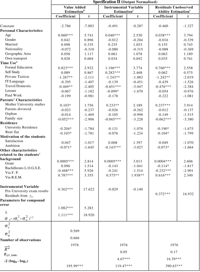
The estimation results of this model are presented in the first column of Table 4. The results are dramatic in their comparison to the stochastic frontier estimation in Table 3. The most important finding is that self study time is now insignificant and the included y_i0 variable gives a γ estimate of .362. This suggests that when ability is included as a proxy by y_i0 the impact of more self study time is negligible. The continued importance of formal study time implies that the only (decision variable) input which matters in terms of student performance is the impact of time in lectures and classes. This would suggest that ability directly constrains student performance and that this is largely unaffected by extra time in self study.

Instrumental Variables Estimation

Another estimation solution which is often adopted in the case of measurement error or endogenous variables is the technique of instrumental variables. This technique requires us to find correlates (X_i0 ), of y_i0 which are not correlated with u_i0or y_i1. Formally we can write the model as:

0 0 ) / ( 0 ) / ( 1 1 0 0 1 1 1 1 = = = Ε = Ε i i i i i i T u X u µ δ µ δ 0 i

X significantly correlated with y_i 0

i

X are valid exclusion restrictions from (7) 0

i

u and u_i1uncorrelated The procedure consists of estimating (6):

0 0 ' 0 0 0 i i i

X

u

y

=

α

+

β

+

compute predicted values of yi0 :

0 ' 0 0 0

ˆ

ˆ

ˆ

α

X

β

y

=

+

1 1 1 1 0 0 1 ' 1 1 1 i

ˆ

X

y

T

u

y

=

α

+

β

+

γ

+

δ

µ

+

π

+

The results obtained from the first step of the instrumental variable procedure can be seen in Appendix C (Table C3). We report different specifications in order to control the problems stemming from the correlation among different personal and parents’ characteristics (specification IV seems to be the most satisfactory). The major conclusion from this table are that those students who attend private Secondary Schools show higher pre-university academic achievements, and those attending Bachillerato L.O.G.S.E. get worse pre-university exam results than reported by students who attended the old Bachillerato (B.U.P.). The estimated values for the instrumental variable (pre-university exam results) are incorporated into the second stage of the procedure (i.e. in the base specifications showed in Tables 2 and 3). The coefficient estimates from the second stage of the instrumental variable procedure are reported in Table 4.

The major conclusion from this table is that the results for all the variables are virtually identical to those shown in Tables 2 and 3. Therefore there is little evidence of possible biases in previous estimations.

Our first step estimation results used in computing the IV of y_i0 in Table 4 are included in Specification V in Table C3 in the Appendix C. We performed the Bound et al. (1995) tests which suggested that the instruments we used are valid with a F statistic of 14.15 which is significant at the 1% level. The partial r squared is 0.0259. None of the regressors used in this specification are significant in explaining university exam results. Superficially these results suggest that the IV approach may be a suitable technique for handling the problem of the endogeneity of y_i0 in the y_i1 equation. We can also see this as y_i0 being an imperfect proxy of µ_i0with measurement error. In either case the technique of IV estimation would be justified32. The results of this estimation are presented in the second column section of Table 4. They show us that the IV variable is not significant in the determination of y_i1. This conclusion is supported in the Hausman-Wu mis-specification test which shows that H₀, the hypothesis that there is no systematic difference between the regression coefficients in the original model

32

Note that the estimation of (12) is by OLS since the IV procedure is only strictly valid for this stimation technique.