Combining Feature Reduction and Case
Selection in Building CBR Classifiers
Yan Li,
Student Member,
IEEE, Simon C.K. Shiu,
Member,
IEEE, and Sankar K. Pal,
Fellow,
IEEE
Abstract—CBR systems that are built for the classification problems are called CBR classifiers. This paper presents a novel and fast approach to building efficient and competent CBR classifiers that combines both feature reduction (FR) and case selection (CS). It has three central contributions: 1) it develops a fast rough-set method based on relative attribute dependency among features to compute the approximate reduct, 2) it constructs and compares different case selection methods based on the similarity measure and the concepts of case coverage and case reachability, and 3) CBR classifiers built using a combination of the FR and CS processes can reduce the training burden as well as the need to acquire domain knowledge. The overall experimental results demonstrating on four real-life data sets show that the combined FR and CS method can preserve, and may also improve, the solution accuracy while at the same time substantially reducing the storage space. The case retrieval time is also greatly reduced because the use of CBR classifier contains a smaller amount of cases with fewer features. The developed FR and CS combination method is also compared with the kernel PCA and SVMs techniques. Their storage requirement, classification accuracy, and classification speed are presented and discussed.Index Terms—Case-based reasoning, CBR classifier, case selection, feature reduction, k-NN principle, rough sets.
æ
1
I
NTRODUCTIONC
ASE-BASEDReasoning (CBR) is a reasoning methodology that is based on prior experience and examples. It retains a memory of previous problems and their solutions, and solves new problems by reference to this knowledge [1], [2]. When a CBR reasoner is presented with a problem (or called an unseen case), it searches its memory of past cases (called the case base) and attempts to find a case that most closely matches the current unseen case. CBR systems have been widely used in prediction and classification [3], [4], [5], [6], [7], knowledge inference and evaluation [8], [9], among others [10], [11]. In these applications, CBR systems that are built for the classification problem—to determine whether or not an object is a member of a class, or which of several classes it may belong to—are called CBR classifiers. CBR systems usually require significantly less knowledge acquisition than rule-based systems since they involve the collection of a set of past experiences without requiring the extraction of a formal domain model from these cases. In this paper, we present a novel and fast approach which builds efficient and competent CBR classifiers by combining the feature reduction (FR) and case selection (CS) processes. FR, the first step in building CBR classifiers, is the process of removing noninformative features or of preser-ving informative ones. The related work to FR involves reduction of pattern dimensionality through feature selec-tion or feature extracselec-tion methods [12]. Principle compo-nent analysis (PCA) [13], [14] is one of the widely usedunsupervised techniques to detect the data structure and reduce the data dimensionality. Recently, a nonlinear version of PCA, called kernel PCA (KPCA) [15], was used to capture the dominant nonlinear features of the original data. It transformed the data to a high-dimensional feature space and obtained a set of transformed features rather than a subset of the original features [16]. Since it is based on the data variance, this technique can only be used to deal with numerical features. There are also some other FR methods that have been used in very special applications, such as Shrunken centroid [17] which is about DNA microarray analysis.
Another often used approach in FR is rough sets [18], [19], the effectiveness of which have been demonstrated in many different domains [20], [21], [22], [23], [24]. Rough sets allow the most informative features to be detected and then selected through the reduct computation. Different from PCA, this approach is supervised and selects a subset of the original features. Furthermore, PCA is used primarily for numerical features, and rough sets are often used on symbolic features. There are two main groups of rough set-based FR methods: discernibility function-based [25] and attribute dependency-based [26]. Such methods, how-ever, are computational intensive, i.e., in the former, during the generation of the discernibility matrix and in the latter, during the discovery of the positive regions.
To reduce the computational load inherent in these methods, Han et al. [27] proposed a relative attribute dependency approach, which can generate a reduct by counting the distinct rows in the subdecision tables produced from the attribute subsets. In this approach, however, the information systems are always assumed to be consistent, which is not necessarily true in real-world applications. To overcome this problem, we will introduce a new concept of approximate reduct in this paper. The concepts of dispensable and indispensable attributes; reduct . Y. Li and S.C.K. Shiu are with the Department of Computing, The Hong
Kong Polytechnic University, Hung Hom, Kowloon, Hong Kong. E-mail: {csyli, csckshiu}@comp.polyu.edu.hk.
. S.K. Pal is with the Machine Intelligence Unit, Indian Statistical Institute, Kolkata, 700 108, India. E-mail: [email protected].
Manuscript received 16 Nov. 2004; revised 25 Apr. 2005; accepted 8 Sept. 2005; published online 18 Jan. 2006.
For information on obtaining reprints of this article, please send e-mail to: [email protected], and reference IEEECS Log Number TKDE-0411-1104.
and core are also modified. Using these extended concepts, we then develop a fast rough set-based approach to find the approximate reduct. Our FR approach can be considered as a generalization of the original attribute dependency-based or discernibility function-based techniques, which is achieved by introducing a consistency measurement among reducts. The computational complexity of this approach is linear with respect to the number of attributes and cases. Furthermore, the consistency measurement can be used to control the size of the feature set.
After FR comes CS. Like FR, CS is economical. The main objective of the CS process developed in this research is to identify and remove redundant and noisy cases. If two cases are the same (i.e., case duplication) or if one case subsumes another case, one of the cases duplicated or subsumed cases are considered to be redundant. They can be removed from the case base without affecting the overall problem-solving ability of the CBR system. The meaning of subsumption is as follows: Given two casesepandeq, when
caseepsubsumes caseeq, caseepcan be used to solve more
problems thaneq. In this case,eqis said to be redundant. On
the other hand, the definition of noisy cases is very much dependent on how we interpret the data distribution regions, and their association with the class labels. Accord-ing to Brighton and Mellish [28], there are two broad categories of class structures: the classes are defined by 1) homogeneous regions or 2) heterogeneous regions. In this paper, we only consider the first category of data distribu-tion. Based on the assumption that similar problems should have similar solutions, we define noisy cases as those that are very similar in their problem specifications yet propose different (or conflicting) solutions.
CS schemes are traditionally based on the k-NN
principle, e.g., the Condensed Nearest Neighbor Rule (CNN) [29] and the Wilson Editing method [30]. There are several variations of the CNN and Wilson Editing method [31], [32], [33]. These methods have been shown to be very useful for identifying and removing noisy cases because they closely examine thek-nearestneighbors of each case. In this paper, they are referred to ask-NN-basedmethods.
Another recent approach that has been widely used in CS is based on the concepts of case coverage and case reachability.Coverageof a case is the set of target problems (i.e., cases) that this case can be used to solve. The
reachabilityof a target problem (i.e., a case) is the set of all cases that can be used to solve the target problem. These two concepts are very useful for identifying redundant cases because they examine the problem-solving ability of each case. Based on these two concepts, some algorithms are developed in [34], [35], [36], [37]. Other CS approaches include density-based [38], [39] and prototype-based techniques [40], [41], [42]. This research constructs and compares different case selection approaches based on the similarity measure and the concepts of case coverage and reachability, which are closely related to the k-NN-based
methods.
Case generation is another alternative approach for reducing the size of the case base. New cases (prototypes) can be generated instead of selecting a subset of cases from the original case base. These generated new cases have
lower dimension than that in the original case base, for example, the fuzzy-rough method in [43] generated cases of variable dimensions of lower size. On the other hand, the support vectors produced by SVM [44] can be considered as cases selected as a subset of the original case base. Recently, SVM ensemble which consists of several SVMs [45], [46] is proposed to expand the correctly classified area by each individual SVM.
In these CS methods, the issue of feature importance (weight) should be considered in computing the similarity, k-NNs, case-coverage and case-reachability. These weights are usually obtained using machine learning methods, such as decision tree generation [47], or neural network training [2]. However, this transforms the feature weighting information into a set of rules or a trained neural network making them unsuitable for calculating similarity and adaptation on unseen cases. Other problems of using these machine learning methods include the difficulty of deter-mining a feature evaluation function and the requirement of much training effort due to the presence of noninformative features in the training process.
In this paper, the feature importance is addressed by the reduct generation. The features in the selected reduct are regarded as the most important ones, and the other features are regarded as irrelevant. The reduct computation does not require any domain knowledge, and the computation complexity is only linear with respect to the number of attributes and cases. After incorporating the FR and CS, the case representation should still be the same as that of the original case base. That is, each case is described by a set of features (subset of the original feature set) and a class label. This form of knowledge representation is easier to under-stand and more convenient for use in CBR reasoning.
In order to find the “best” subset of features (i.e., the set of features which can achieve the highest classification accuracy) that could be used by the CS process, we generate different approximate reducts in FR by fine-tuning the value of the consistency measurement (i.e., parameter) of the subfeature set. This allows the size of the approximate reduct to be controlled, and the “best” subset of features to be obtained.
This work makes three main contributions. First, based on the relative attribute dependency among features, we develop a fast rough-set approach for computing the approximate reduct instead of the exact reduct. Second, we construct and compare four different similarity measure-based case selection methods. Finally, the CBR classifiers built using a combined FR and CS approach reduces both the burden of training and the need to acquire domain knowl-edge. The experimental results show that our proposed FR and CS methods, used individually or in combination, can preserve and even improve the classification accuracy while at the same time reduce the storage space.
The reminder of the paper is organized as follows: Section 2 presents the fast rough set-based FR approach. Section 3 provides four CS algorithms and their rationales. Section 4 explains the importance of FR in CS and the steps for combining them. Section 5 presents and analyses experimental results on both the individual and synergistic performance of the FR and CS methods. Some comparisons
are also made between the developed FR and CS methods and the combination of KPCA and SVMs techniques. Section 6 provides the conclusions and discussions.
2
F
ASTR
OUGHS
ET-B
ASEDF
EATURER
EDUCTIONA
PPROACHThe purpose of FR is to identify the most significant attributes and eliminate the irrelevant ones to form a good feature subset for classification tasks. It reduces the running time of classification processes and increases the accuracy of classification models. In this paper, we focus on the rough set-based FR methods.
First, the following provides some definitions and properties of rough sets.
LetIS¼ ðU; A; fÞbe an information system, whereUis a finite nonempty set ofNobjectsfx1; x2;. . .; xNg;Ais a finite
nonempty set ofn attributes (features)fa1; a2;. . .; ang; fa:
U !Va for any a2A, where Va is called the domain of
attribute a. A decision table is an information system DT ¼ ðU; A[ fdg; fÞ, where d is the decision attribute, d 62 A.
Definition 1 (Indiscernibility Relation). Each subset of attributes BA determines an equivalent relation, called indiscernibility relationINDðBÞon
U:INDðBÞ ¼ fðx; yÞ 2UUj8a2B; faðxÞ ¼faðyÞg:
Definition 2 (Dispensable and Indispensable Attributes).
An attributeais dispensable in anIS, if INDðA fagÞ ¼INDðAÞ; otherwise,ais indispensable inIS.
Definition 3 (Reduct). A subattribute set BA is called a reduct ofAif it is the set of indispensable attributes in theIS, i.e., ifB¼ fajINDðA fagÞ 6¼INDðAÞ; a2Ag, thenBis a reduct ofA.
Definition 4 (Discernibility Matrix [25]). The discernibility matrix (DM) of anIS which has n objects is a nn matrix represented byðdmijÞ, where
dmij¼ fa2A:faðxiÞ 6¼faðxjÞgfor i; j¼1;2;. . .; n:
Based on these definitions, it requires a considerable effort for the discernibility function-based reduct generation methods to compute the discernibility matrix. For example, if there arenobjects in theIS,mattributes inA[ fdg, the computation complexity of these methods isOðn2mÞ. To address this problem, Han et al. [27] have developed a reduct computation approach based on the concept of relative attribute dependency. Given a subset of condition attributes, B, the relative attribute dependency is a ratio between the number of distinct rows in the decision table corresponding toBonly and the number of distinct rows in the decision table corresponding to B together with the decision attributes, i.e., B[ fdg. The larger the relative attribute dependency value (i.e., close to 1), the more useful is the subset of condition attributesBin discriminating the decision attribute values. If this value is equal to 1, each
distinct row in the decision table corresponding toBmaps to a distinct decision attribute value.
Some further concepts [27] are defined as:
Definition 5 (Projection). Let PA[D, where D¼ fdg. The projection ofU onP, denoted byQPðUÞ, is a subtable of U and is constructed as follows: 1) Remove attributes inA[ DP and 2) merge all indiscernible rows.
Definition 6 (Consistent Decision Table). A decision table DT on U is consistent when 8x;y2U; if fdðxÞ 6¼fdðyÞ, d2D, then9a2Asuch thatfaðxÞ 6¼faðyÞ.
Definition 7 (Relative Dependency Degree).LetBA,A be the set of conditional attributes. D is the set of decision attributes. The relative dependency degree ofBwith regard to Dis defined asDB,
DB¼
jBðUÞj
jB[DðUÞj;
where jXðUÞj is the number of equivalence classes in
U=INDðXÞ.
The relative dependency degree D
B implies how well
subset B discerns the objects inU relative to the original attribute setA. It can be computed by counting the number of equivalence classes induced by B and B[D, i.e., the distinct rows in the projections ofUonBandB[D. Based on the definition of the relative dependency degree, dispensable and indispensable attributes are defined as: Definition 8 (Dispensable and Indispensable Attributes).
An attributea2Ais said to be dispensable inAwith regard toD ifD
Afag¼DA; otherwise,ais indispensable inA with
regard toD.
According to Definitions 6, 7, and 8, Theorem 1 can be obtained.
Theorem 1.IfUis consistent,BAis a reduct ofAwith regard toD, if and only ifD
B¼DA ¼1and for 8QB; QD6¼DA.
(See [27] for the proof.)
In order to compute the reduct quickly, we use Definitions 7 and 8 (relative dependency degree, dispen-sable and indispendispen-sable attributes) and Theorem 1. Theo-rem 1 gives the necessary and sufficient conditions for reduct computation and implies that the reduct can be generated by only counting the distinct rows in some projections.
In Theorem 1, U is always assumed to be consistent, which is not necessarily true in real-life applications. In order to find approximate reducts rather than the exact reducts, we relax this condition. The use of a relative dependency degree in reduct computation is extended to inconsistent information systems. Some new concepts, such as the -dispensable attribute, -indispensable attribute, -reduct (i.e., approximate reduct), and -core are intro-duced to modify the traditional concepts in the rough set theory. The parameter is used as the consistency measurement to evaluate the goodness of the subset of attributes currently under consideration. It can also deter-mine the number of attributes which will be selected in the
generated approximate reduct. These are explained as follows:
Definition 9 (-dispensable attribute and -indispensable
attribute). If a2A is an attribute that satisfies D
AfagAD, a is called a -dispensable attribute in A.
Otherwise, a is called a -indispensable attribute. The parameter,2 ½0;1, is called the consistency measurement.
Definition 10 (-reduct=approximatereduct and-core).B is called a -reduct or approximate reduct of conditional attribute set A if B is the minimal subset of A such that DB AD. The -core of A is the set of -indispensable
attributes.
The consistency measurement represents how consis-tent the subdecision table (with respect to the considered subset of attributes) is relative to the original decision table (with respect to the original attribute set). It also reflects the relationship of the approximate reduct and the exact reduct. The larger the value of , the more similar is the approximate reduct to the exact reduct computed using the traditional discernibility function-based methods. If¼
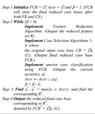
1 (i.e., attains its maximum), the two reducts are equal (according to Theorem 1). The reduct computation is implemented by counting the distinct rows in the subdeci-sion tables of some subattribute sets. controls the end condition of the algorithm and, therefore, controls the size of reduced feature set. Based on Definitions 9 and 10, the first rough set-based FR algorithm in our developed approach is given in Fig. 1.
In some domains, the order for selecting attributes in the reduct must be considered carefully. For example, when dealing with text documents, there are hundreds or thousands of keywords which are all regarded as attributes. If the order is randomly selected or if one simply makes use of the order in which keywords appear in a text document, the most informative attributes may not be selected initially during reduct computation. Therefore, the end condition D
R > in Algorithm 1 cannot be satisfied quickly. It should
also be borne in mind that the final attribute set may consist
of many noninformative features. This issue is addressed by computing the significance value of each attribute. These significance values are used to guide the attribute selection sequence. Details are given in Algorithm 2 (see Fig. 2).
The computation complexities of the feature reduction Algorithms 1 and 2 areOðnmÞ, wheremis the number of features inA[D,nis the number of objects inU.
3
C
ASES
ELECTIONA
PPROACHIn this section, we present four CS algorithms that are based on the similarity measure but that use of the case similarity in different ways. Algorithm 1 first selects cases having a large coverage and then, if the two cases have a similar coverage, selects the one with the smaller reachability set. CS Algorithm 2 directly selects cases according to measure-ments of case similarity. The CS Algorithms 3 and 4 are formed by incorporating the k-NN principle into CS Algorithm 1 and CS Algorithm 2, respectively.
The four CS approaches each has its own rationale. For CS Algorithm 1, the similarity measure is used to compute a case’s coverage and reachability values which can be interpreted as an measurement of its significance with respect to all other cases. A case is considered to be important if it “covers” many similar cases (with a similarity value greater than a threshold ) all belonging to the same class. Here, is the similarity threshold between a particular case and its nearest boundary case. Since the cluster centers (cases) often have large coverage sets and the boundary cases have small coverage sets, this CS algorithm tends to select the cluster centers and remove the boundary cases.
CS Algorithm 2 assumes that redundant cases can be found in densely populated case clusters, with the similarity measure being used to describe the local density around a case. The more densely populated the cluster, the more redundant cases should be removed. A threshold can then be set up to determine the number of cases which should be deleted. Assume ep is a case which has been
already selected. A case eq is considered to be redundant
and should be removed if the similarity of ep and eq is
greater than the given threshold and the classification label ofepis the same as that ofeq. As they tend to have different
class labels from their neighbor cases, boundary cases will not be removed. Therefore, a number of representative interior cases and the boundary cases are preserved. This algorithm is fast, and it is suitable for case bases with high densities. However, both CS Algorithms 1 and 2 are vulnerable to noisy cases. The noisy cases mislead the computations of case coverage and reachability in the first CS algorithm, and they are often recognized as boundary cases which play an important role in the second CS algorithm. In order to solve this problem, the k-NN
principle is incorporated into the CS Algorithms 1 and 2 to first detect and remove noisy cases, thereby forming Algorithms 3 and 4. Based on the assumption that similar cases should have similar solutions, noisy cases are defined as cases having different class labels from the majority voting of theirk-nearestneighbors. After the noisy cases are removed, CS Algorithms 1 and 2 are applied to remove the redundant cases. In this way, both noisy and redundant cases can be deleted from the case base.
Before providing a detailed description of the four CS algorithms, we shall define some related concepts. Assume there is a case baseCB, the condition attribute set is A, the decision attribute set is D. The concepts of case coverage and case reachability are defined as follows: Definition 11.Coverage Set of a case e is defined as
CoverðeÞ ¼ fe0je02CB; simðe; e0Þ> ; dðeÞ ¼dðe0Þg; where is the similarity computed between case e and its nearest boundary case (the cases which have different class label ofe);dis the decision attribute inD.
Here, the coverage set of a caseeis the set of cases which fall in the disc centerd atewith radius. We assume there are only one decision attribute d. It is straightforward to extend the definition to a situation with multiple decision attributes.
Definition 12.Reachability Set of a case can be derived from the Definition 11:
ReachðeÞ ¼ fe0je02CB; e can be covered by e0g: These definitions are illustrated in Fig. 3, where ee is the nearest boundary case of cases e1 and e2; ee0 is the
boundary case of e3 and e4. The dotted circle centerd at a
case represents the coverage set of this case. According to Definitions 11 and 12, we have
Coverðe1Þ ¼ fe1g; Coverðe2Þ ¼ fe1; e2g; Coverðe3Þ ¼ fe1; e2; e3; e4g; Coverðe4Þ ¼ fe4g;
and
Reachðe1Þ ¼ fe1; e2; e3g; Reachðe2Þ ¼ fe2; e3g; Reachðe3Þ ¼ fe3g; Reachðe4Þ ¼ fe3; e4g:
The implication of the concepts of case coverage and reachability is that the larger the coverage set of a case, the more significant the case because it can correctly classify more cases based on the k-NN principle. In contrast, the larger the reachability set of a case, the less important the case in the case base because it can be reached by more existing cases. One focus of this paper is the preservation of the competence (the number of cases the case base can cover) of the case bases. We attempt to build an algorithm (see Fig. 4) for selecting a subset of cases that would preserve the overall competence as compared to the original entire case base.
Since the algorithm involves the computation of cover-age set and reachability set for each case in the original case base, the computation complexity of this algorithm is
Oðmn2Þ, wheremis the number of condition attributes
in A; n is the number of cases in the case base. Case selection Algorithm 2, shown in Fig. 5, is much faster since it requires only one pass of the case base to compute the similarity between each two cases. Algorithm 2 is totally similarity-based. If the similarity between a caseeand the current caseeis larger than a given thresholdand they are with the same class label, e will be considered as redundant and eliminated from the case base. This algorithm is suitable to the case bases with high density cases, while the CS Algorithm 1 can be used on both sparse and dense cases. Notice that, the larger the parameter, the more cases are selected by this algorithm. The value ofcan be determined either by the predefined size of the selected case base, or by the required classification accuracy.
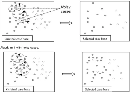
Based on the concepts of coverage and reachability, case selection Algorithm 1 could remove not only the redundant cases but also the noisy cases due to the small coverage sets of the noisy cases (see Fig. 6). However, the effectiveness of Fig. 3. The CoverageSet and ReachabilitySet.
CS is still degraded by the existence of noisy cases. Cases located near the noisy cases tend to have smaller coverage sets than do other cases. As a result, cases close to noisy cases would be selected less often, which may lead to the loss of important information. As shown in Fig. 7, case selection Algorithm 2 tends to eliminate redundant cases but was not able to effectively deal with noisy cases. A noisy caseemay be regarded as a boundary case. Since its class label could not be predicted by the cases which satisfy simðe; eÞ> , it could not be removed. This would result in the preservation of noisy cases (see Fig. 7) and the selection of an unsatisfactory case base.
To tackle the mentioned problems with case selection Algorithm 1 and Algorithm 2, the k-NN principle is incorporated to delete both the noisy cases and the redundant cases. Based on the similarity computation
between cases, thek-NNprinciple is first used to find out the noisy cases. A case is said to be a noisy case if it cannot be correctly classified by the majority of its k-nearest
neighbors. Notice that, when the value k increases, the possibility of a case being a noisy case decreases, and vice versa. In this paper,kis equal to the small odd number, 3. After the noisy case removal, the case selection Algorithms 1 and 2 are then applied to further eliminate the redundant cases. The CS methods which incorporate thek-NNprinciple in the CS Algorithms 1 and 2 are given as case selection Algorithms 3 and 4 (see Fig. 8).
4
C
OMBININGF
EATURER
EDUCTION ANDC
ASES
ELECTIONIn most existing CS methods, as a first step, one computes the similarity between cases using all features involved and then the similarities are used to compute k-nearest
neighbors, case coverage sets and reachability sets. The feature importance can be determined in advance with domain knowledge; or the feature weights are learned by training some models. Each method, however, has some limitations which offer challenges to both FR and CS.
When the feature weights must be determined in advance using required domain knowledge, the knowl-edge is obtained either by interviewing experts—which is labor intensive—or is extracted from the cases—which adds to the burden of training. Similarly, when feature weights must be learned using models such as neural networks or decision trees, the burden of training is again not trivial and, even after training these models, the case representation is then in the form of a trained neural network or a number of rules, which is not convenient for directly retrieving similar cases from a case base for the unseen cases.
Fig. 5. Case selection Algorithm 2.
Fig. 6. Case selection Algorithm 1 with noisy cases.
We address these problems by combining the fast rough set-based FR approach with the CS algorithms. Feature importance is taken into account through reduct generation. The features in the reduct are regarded as the most important while other features are considered to be irrelevant. Reduct computation does not require any domain knowledge and the computational complexity is only linear with respect to the number of attributes and cases. After combining the FR method and CS algorithms, the case representation is still the same as that of the original case base. This form of knowledge representation is easier to understand and more convenient for retrieving unseen cases. Furthermore, since only the features in the reduct are involved in the computations in the CS algorithms, the running time for case selection is also reduced.
For the CBR classifiers, there are three main benefits from combining FR with CS: 1) classification accuracy can be preserved or even improved by removing noninforma-tive features and redundant and noisy cases, 2) storage requirements are reduced by deleting irrelevant features and redundant cases, and 3) the classification decision response time can be reduced because fewer features and cases will be examined when an unseen case occurs.
In this work, we will propose two ways to combine FR and CS based on different definitions of a “best” subfeature set (approximate reduct) R. The first method—called an “open loop”—applies the FR and CS sequentially and only once. The best approximate reduct is identified after applying FR alone. In contrast, the second method can be regarded as an “close loop,” which integrates FR and CS in an interactive manner, determining the best approximate reduct after applying both FR and CS approaches. The interaction of FR and CS is reflected in the identification of the suitablevalue.
In the first, “open loop” method, the “best” approximate reduct R is defined as the approximate reduct which can achieve the highest accuracy after applying only the FR process. Such a best approximate reduct can be generated by iteratively tuning the value of the consistency measure-ment . For example, we start from the exact reduct with ¼1, and in each iteration reduce using a given parameter¼0:01. When the classification accuracy attains its maximum after applying FR alone, the approximate reduct is selected asR. In the following CS process,R is used to detect redundant and noisy cases. In the second, “close loop” method, the “best” subfeature set is defined as the approximate reduct which can achieve the highest accuracy after applying both FR and CS.R is determined much as in the first method. The value of consistency
measurement is modified with step length until it attains its maximum classification accuracy. Theoretically speaking, the “best” approximation reduct found using the second method is not necessarily the same as that found using the first method. The two combination methods are described as follows (see Fig. 9 and Fig. 10):
Obviously, the second combination method, RFRCS2, requires more computational effort because the “best” approximate reduct depends on both FR and CS processes.
5
E
XPERIMENTALR
ESULTSIn this section, we test our proposed FR algorithms, CS algorithms, their combinations and provide compar-isons with KPCA and SVMs techniques. To demonstrate their effectiveness, we use three main evaluation indices: storage requirement, classification accuracy, and classifica-tion speed. In Secclassifica-tion 5.1, storage is the percentage of preserved features after FR process; in Section 5.2, storage is the percentage of selected cases after CS process. The Fig. 8. Case selection Algorithms 3 and 4.
classification accuracy is the percentage of the unseen cases which can be correctly classify. The classification speed is used in Section 5.3.2 to examine the efficiency of the built classifier using the FR and CS combinations. In Section 5.4, all these evaluation indices are considered in the compar-isons between our approach with the KPCA and SVMs.
The experiments used four real-life data sets:
1. House-votes-84 database [48]. It contains a total of 435 cases and 17 Boolean valued features.
2. Text document sets (Texts 1-8). It is composed of eight text document sets randomly sampled from Reuters21578 [49]. The number of documents ranges from 40 to 1,578, and the number of distinct words (i.e., condition attributes) ranges from 150 to 2,018.
3. Mushroom Database [48]. There are 8,124 samples and 23 nominally valued features.
4. Multiple Features [48]. This data set consists of numerical features of handwritten numbers from
“0” to “9.” There are a total of 2,000 samples, 649 attributes, and 10 classes. This data set is used to compare our developed FR and CS methods with the combination of KPCA and SVMs techniques. 5.1 Rough Set-Based Feature Reduction
In this section, we test and analyze the feature reduction capability of the rough set-based algorithm proposed in Section 2. FR Algorithm 2 is used on the Text data sets, and FR Algorithm 1 is used for other data sets.
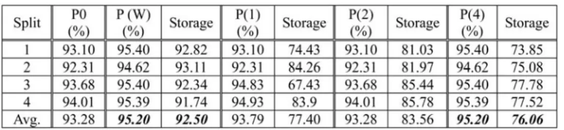
House-votes-84. This data set is tested using four splits: randomly selecting 20, 30, 40, and 50 percent, as the testing data (unseen data); the corresponding left data are used as the training data. The four splits are denoted as Split 1-4. Table 1 shows the reduced storage requirement and the classification accuracy with differentvalues.
Table 1 provokes two observations: 1) The classification accuracy is improved after the rough set-based FR with almost all of the usedvalues. 2) The accuracy attains most of its maximums for the four splits when ¼0:95 (see Table 1). This is why the value is set at 0.95 in Table 2. Here, P0 represents the original accuracy with the whole data set, while P(FR) denotes the accuracy with the reduced feature set after applying FR Algorithm 1 (Section 2).
Text data sets. Here, the FR Algorithm 2 is applied. We randomly select 80 percent documents in each text data set as the training data and the remaining 20 percent is used as the testing data. In the FR Algorithm 2, the significance of each feature is evaluated by its frequency of occurrence.
Table 3 shows that the storage requirements for all the eight data sets fall significantly, and the accuracy using reduced feature set is preserved for Text2, Text3, and Text6 and even improves for Text1, Texts4-5. For Texts7-8, the accuracy decreases a little due to the reduction of features. Since the accuracy attains its maximum when¼1, here is set to be 1.
Summary. After applying the fast rough set-based FR method to House-votes data and texts 1-8, the feature set is substantially reduced and the classification accuracy is preserved or even improved. Tables 1, Table 2, and Table 3 show that the improvement in classification accuracy is 3.06 percent for House-votes-84 and 3.77 percent for the text data sets. The size of the feature set decreases from the original 100 percent to 53.13 percent for house-votes-84 and 14.11 percent for text data sets.
Fig. 10. The RFRCS 2 Algorithm.
TABLE 1
5.2 Case Selection
The CS algorithms developed in Section 3 are applied to the real-life data sets and compared with the traditional Wilson Editing. Note that the generation method of the training data and testing data is the same as that in Section 5.1 for each data set.
Table 4 and Table 5 demonstrate the reduced storage and improved accuracy when using different CS algorithms. P(W), P(1), P(2), and P(4) represent the classification accuracy using Wilson Editing, case selection Algorithms 1, 2, and 4, respectively.Notice that the results of Algorithm 3 are very similar to those of Algorithm 1. Due to space limitations, they are not included in Table 4 and Table 5 and related results in the following sections. Unlike in Section 5.1, in this section “storage” means the proportion of cases which are selected in the final case base. In case selection Algorithm 2, the parameter¼0:99.
Table 4 (the house-votes data) shows that after case selection, all the CS algorithms were able to reduce cases while preserve or even improve classification accuracy. The Wilson Editing and case selection Algorithm 4 attain greatest accuracy while Algorithm 4 has a more powerful capability to reduce useless cases than other algorithms do. Table 5 shows the results for the text data sets. Algorithm 2 is most accurate. Algorithm 4 produced the smallest reduced case base with respect to the number of cases. To summarize, both Table 4 and Table 5 show results for Algorithm 4 that are satisfactory in terms of both classifica-tion accuracy and storage requirements after the case selection.
5.3 Combining Feature Reduction and Case Selection
In this section, we will discuss some experiments using RFRCS1 and RFRCS2 (Section 4) that were conducted to show the positive impact of the rough set-based FR method on the CS algorithms. The two main evaluation measure-ments are still storage and accuracy. Comparisons are made based on thek-NNclassifier, using different CS algorithms in combination with FR. Here, k is set to a small odd number, 3. The data splitting methods of training data/ testing data for all the involved data sets are the same as those in Sections 5.1 and 5.2.
In this section, let P(F+W) denote the classification accuracy of the combination of the rough set-based FR and Wilson Editing; and P(F+1), P(F+2), P(F+3), P(F+4) that of case selection Algorithms 1 to 4. The final reduced case base is the case base containing the reduced feature set and the selected cases. Since RFRCS2 requires a greater computational effort, in this section, we mainly conduct the experiments using the algorithm RFRCS1.
5.3.1 RFRCS1: Storage Requirement and Classification Accuracy
House-votes-84. On this data set, RFRCS1 incorporates the proposed fast rough set-based FR approach into the CS algorithms. From Table 6, the combined algorithms are more accurate and require less storage space than the approaches that make use of individual CS algo-rithms alone.
Algorithms (F+W) and (F+4) are shown to be most accurate. The (F+4) algorithm also has the best classification accuracy and the most reduced storage requirement. This is because the CS Algorithm 4 is able to reduce cases more effectively than algorithm that use Wilson Editing (Table 4). TABLE 2
Storage and Accuracy Using¼0:95on House-Votes-84
TABLE 3
Reduced Storage and Improved Accuracy When Applying¼1to Text Data
TABLE 4
We can conclude that the fast rough set-based FR approach with CS Algorithm 4 is superior to other FR and CS algorithms used either individually or in combination.
Text data sets. This section examines the impact of FR on CS using the text data sets. Table 7 displays the text data set results. They are similar to those for the house-votes data set, except that the improvement in accuracy is much greater after incorporating FR to CS.
Mushroom data. We found that only CS Algorithm 1 was able to remove cases. This is because the Mushroom data is sparse and other CS algorithms are suitable to the highly dense data. The classification accuracy of the FR approach was the same as the original accuracy using the entire case base, 1. Table 8 shows the impact of feature reduction on CS Algorithm 1. On average, the classification accuracy after applying the combination of FR and the
CS algorithm 1 increases by 9.3 percent. Here, the storage is the percentage of cases which need to be stored in the final reduced case base after applying the CS Algorithm 1. For TABLE 5
Case Selection Using Text Data Sets
TABLE 6
Applying RFRCS1 to House-Votes-84 (¼0:95)
TABLE 7
Applying RFRCS1 to Text Data Sets (¼1)
TABLE 8
the FR in algorithm (F+1), is set to be 1. There are five features in the generated reduct so the storage of the feature set is 22.7 percent of the original feature set.
To conclude, when RFRCS1 is applied, the results of almost all of the data sets and of all of the proposed CS algorithms are positive. The classification accuracy and storage requirement show a notable improvement: When the CS algorithms are applied to the house-votes-84 data, the average increase in accuracy is 1.91 percent (Table 6). Applied to the text data sets, it is 4.95 percent (Table 7), and applied to the mushroom data set it is 9.33 percent (Table 8). These improvements in accuracy are, respectively, achieved only with 51.13 percent (Table 2), 14.9 percent (Table 3), and 22.73 percent of the original features for the three data sets. The combination of the rough set-based FR approach with the CS Algorithm 4, (F + 4), is the most promising algorithm in terms of both accuracy and storage.
5.3.2 Classification Efficiency of RFRCS1
This section describes some experiments using RFRCS1 carried out to determine the efficiency of case retrieval or unseen case (testing case) classification after reducing both features and cases.
Table 9 shows the average T_FR, T_CS, T0, T, and Ts
using the three data sets. T_FR and T_CS are the average time cost in the FR process and the CS Algorithm 4, respectively. T0 and T are the average time needed to classify one unseen case using the entire original data sets, and using the reduced data set, respectively. Ts¼T0T,
describes the amount of time that is saved for an unseen case classification due to this data compression. T_FR, T_CS, T0, T, and Ts are represented in seconds. The
efficiency of case classification is shown to be improved using the reduced data sets. Although the average saved time of identifying only one unseen case is not notable, it could be significant using all the testing cases. For example, for house-votes-84 data, the total saved time for classifying all the 217 testing cases isð0:03217Þ 6:51seconds. 5.3.3 Storage Requirement and Classification Accuracy
of RFRCS2
In previous sections, we performed some experiments using RFRCS1. The “best” and approximate reduct were determined through only in the FR process. In this section, the RFRCS2 is applied to real-life data, where the most suitable is obtained when the final accuracy attains its maximum after both FR and CS. The experimental results show that the best values found in RFRCS2 are not necessarily the same as those in RFRCS1. Compared with
RFRCS1, using this kind of combination of FR with CS, the classification accuracy is shown to be further improved and/or the storage space could be further reduced.
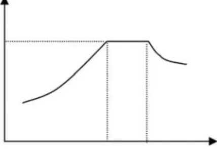
House-votes-84. The most suitablefound for this data set is 0.90, but not 0.95 in RFRCS1. There are seven features (43.75 percent of the original features) in the corresponding approximate reduct. Compared with RFRCS1, the classifi-cation accuracy is preserved using the reduced case base while the number of features is further reduced. Fig. 11 shows the relationship between P(F+4) andvalues. When 2 ½0:90;0:95, the accuracy attains its maximum, 0.977. Since the smaller thevalue, the fewer the features in the corresponding approximate reduct,is set to be 0.90 so that the accuracy can be preserved whereas the number of features is minimum. The similar results could be achieved using other CS algorithms. Table 10 shows the results in detail. Here, “Storage” means the storage requirement with respect to the features instead of the cases; “Max accuracy” is the highest classification accuracy obtained by combina-tions of FR with different CS algorithms. As can be seen in Table 10 using RFRCS2, the maximum accuracies have been preserved and the feature storage requirement decreases by 9.38 percent from 53.13 (using RFRCS1) to 43.75 (using RFRCS2).
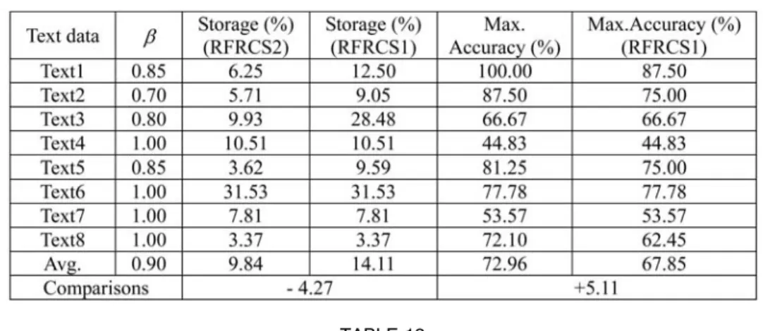
Text data sets. In Section 5.3.1,is set to be 1 for the text data sets. In this section, using the combination method RFRCS2, various bestvalues are found for different text data sets. Table 11 demonstrates that, with these different values, the average required storage space could be further reduced from 14.11 percent to 9.84 percent of the original features, the average maximum accuracy increases by 5.11 percent from 67.85 percent to 72.96 percent.
Mushroom data. After applying RFRCS2, the best in the mushroom data set is the same as in RFRCS1, i.e.,¼1. Therefore, the results of RFRCS2 with respect to the storage TABLE 9
Speed of Case Classification Using RFRCS1
Fig. 11. P(F + 4) versusvalues.
TABLE 10
requirement, classification accuracy are the same as in Section 5.3.1.
Discussions. Using the combination method RFRCS2, the bestvalues which achieve the maximum accuracies after applying both FR and CS can be found for the real-life data sets. Compared with RFRCS1, more computational efforts are required by RFRCS2 because the CS process is involved in tuning thevalues. The accuracy is shown to be preserved (for House-votes-84 and Mushroom data) and even im-proved (for the text data sets) and the storage requirement of the feature set is further reduced (for House-votes-84 and text data sets). The users can choose either RFRCS1 or RFRCS2 to construct the final case base for the CBR classifier. For large case bases, users can select RFRCS1 which has less computational load with still satisfactory accuracy.
5.4 Comparisons: Rough Set-Based FR and CS versus KPCA and SVMs
Some comparisons are made to further demonstrate the effectiveness of our FR and CS methods. In Section 5.4.1, the fast rough set-based FR method is compared with KPCA. In Section 5.4.2, RFRCS1 is compared with the combination of KPCA and SVM ensembles.
The experiment setup is as follows: 1) Data: Since KPCA can only handle numerical data, the data set of Multiple Featuresis used in the experiments. 2) Data splitting: We use the training/testing data sets in the original data ofMultiple Features, which has 1,000 training samples and 1,000 testing samples. 3) Performance evaluation: Four main evaluation indices are used including training time, retrieval time, storage requirement, and classification accuracy. Here, the unit of time is second.
5.4.1 Rough Set-Based FR and KPCA Feature Exaction In order to compare the developed rough set-based FR and KPCA methods, fuzzy discretization [43] is performed before applying rough sets for feature reduction. For the KPCA method, we select polynomial kernels due to the expensive training with RBF kernels.
Table 12 shows the experimental results, where “T_train” is the training time; “T_trans” in KPCA is the required time for testing data transformation on the extracted components. The comparisons are made based on the same number of selected features. It is demonstrated that the KPCA achieves a slightly higher classification accuracy; however, the training time and the transformation time are much more than the training time in rough set-based FR method.
5.4.2 RFRCS1 and the Combination of KPCA and SVMs In this section, RFRCS1 is compared with the combined KPCA and SVM ensembles. Here, the CS Algorithm 4 is used for CS after the FR process. From Table 12, we notice that when 1.87 percent features (i.e., 13 features) are selected, the accuracy attains its maximum. Therefore, value is set as 0.99 and the number of eigenvectors extracted by KPCA is determined as 13. On the other hand, after the feature extraction of KPCA, a transformed data set is obtained which has a lower dimensionality. This new reduced data set is then used in constructing the multiple SVM classifiers. Here, we use the one-against-all method to deal with the multiple class problem, and the final results are combined based on the majority voting rule. Since the data set contains 10 classes, 10 SVMs are constructed and TABLE 11
RFRCS2 with VariousValues on Text Data Sets
TABLE 12
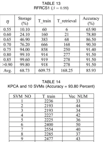
trained in the experiments. Here, we use the Matlab Support Vector Machine Toolbox developed by Gunn [50]. Table 13 and Table 14 show the results of RFRCS1 and the combination of KPCA and SVMs. Here, the “Storage” is the percentage of selected cases; “T_train” is the processing time of the CS method. In RFRCS1, with the increase of value, the storage, training time, retrieval time, and the accuracy also increase. The combination of KPCA and 10 SVMs totally extracts 408 support vectors (prototypical cases), and the classification accuracy is 93.8 percent, which
is slightly higher than the maximum accuracy obtained by rough set-based method, 91.5 percent. However, the total training time of the 10 SVMs is unacceptable. In contrast, the combination of our FR and CS approach cost less processing time and can still achieve satisfactory classifica-tion accuracy.
In RFRCS1, we use thek-NNprinciple to classify unseen cases, where the k value may affect the classification accuracy. Here, we report the results of some testing using different k values in RFRCS1 on the data set of Multiple Features. Let k¼1;3;. . .;pffiffiffin, where n is the number of training samples. It is demonstrated in Fig. 12 that, the accuracy attains its maximum whenk¼3. Therefore, we set k¼3in the experiments in previous sections.
Table 15 shows the comprehensive comparisons in terms of both qualitative and quantitative indices between the developed rough set-based FR and CS approach and the combination KPCA and SVMs. They are based on different rationales and are suitable to different data types. The rough set-based FR is supervised learning while KPCA is unsupervised. The rough set-based FR generates a subset of the original features and KPCA extracts a set of transformed features. The combination of FR and CS is fast while KPCA and SVMs achieve a slightly higher accuracy. Users can choose either of the combination methods based on the used data and their requirements on efficiency and accuracy.
6
C
ONCLUSIONS ANDD
ISCUSSIONSIn this paper, we describe a fast rough set-based FR approach and four similarity-based CS algorithms. In the TABLE 13
RFRCS1 (¼0:99)
TABLE 14
KPCA and 10 SVMs (Accuracy = 93.80 Percent)
SVM_NO: the ID number of the trained SVM classifier; Vec_NUM: the number of generated support vectors. The retrieval time is not listed in Table 14 because it is trivial compared with the training time.
Fig. 12. The effect of k value on accuracy.
TABLE 15
FR approach, the concept of a reduct is generalized to an approximate reduct, which makes the reduct computation faster and more flexible. In some situations, the crisp reduct is the best subset of features in terms of the classification accuracy, e.g., when¼1for the Text data and Mushroom data (Section 5.1). Although the crisp reduct can be obtained by the traditional discernibility function-based methods, the computational complexity has been reduced using our FR approach. In some other situations, the crisp reduct is not the optimal subset of features, e.g., <1for the House-votes-84 (Section 5.1) and the Multiple Features database (Section 5.4). In this paper, the value is determined to optimize the classification accuracy. The developed CS algorithms can remove not only the redundant cases but also the noisy cases. The CS Algorithm 4 and Wilson Editing achieve the highest accuracy, but the former requires lower storage. It can be shown that, compared with using the original case base, higher classification accuracy and less storage space requirement could be obtained with each individual FR and CS algorithm. By combining the FR and CS processes, we could further enhance the accuracy and reduce the storage. Two methods of combination, RFRCS1 and RFRCS2, are developed based on different definitions of the “best” value of the consis-tency measurement.
The experimental results show that the CS Algorithm 4 with the rough set-based FR algorithm, denoted by (F + 4), is the most promising one which has the highest accuracy and the least storage requirement. The enhanced efficiency using the reduced data sets is also demonstrated through the experimental results in Section 5.3.2. Comparisons are made between RFRCS1 and RFRCS2 in Section 5.3.3. RFRCS2 shows higher accuracy and lower storage load but requires more computational efforts. Some comparisons are also made between the rough set-based FR and KPCA, the RFRCS1 and the combination of KPCA and SVMs. These two combination methods have different character-istics, based on which users can select one of them to reduce both the dimensionality and size of data.
There are still some limitations of our developed FR and CS approaches, which may need to be tackled in our future work: 1) We have only considered the case bases which consist of homogeneous data regions, in which the noisy cases are defined as the cases that cannot be correctly classified by their k-nearest neighbors. Therefore, our approach cannot be directly used on case bases containing heterogeneous data regions, which may result in the fact that some useful cases are misclassified as noisy cases. 2) The determination of the parameters, i.e.,in FR andin CS, is empirical and heuristic based during the testing and their best values are data set dependent. 3) The fast rough set-based FR method works better with symbolic data. The numerical data needs to be discretized before applying FR process.
A
CKNOWLEDGMENTSThis work is supported by the CERG research grant BQ-496.
R
EFERENCES[1] J. Kolodner,Case-Based Reasoning.Morgan Kaufmann, 1993.
[2] S.K. Pal and S.C.K. Shiu,Foundations of Soft Case-Based Reasoning.
John Wiley, 2004.
[3] C.C. Hsu and C.S. Ho, “Acquiring Patient Data by an Intelligent Interface Agent with Medicine-Related Common Sense Reason-ing,” Expert Systems with Applications: An Int’l J.,vol. 17, no. 4, pp. 257-274, 1999.
[4] T.W. Liao, “An Investigation of a Hybrid CBR Method for Failure Mechanisms Identification,”Eng. Applications of Artificial Intelli-gence,vol. 17, no. 1, pp. 123-134, 2004.
[5] E. Kalapanidas and N. Avouris, “Short-Term Air Quality Prediction Using a Case-Based Classifier,”Environmental Model-ling and Software,vol. 16, no. 3, pp. 263-272, 2001.
[6] K.E. Emam, S. Benlarbi, N. Goel, and S.N. Rai, “Comparing Case-Based Reasoning Classifiers for Predicting High Risk Software Components,”J. Systems and Software,vol. 55, no. 3, pp. 301-320, 2001.
[7] J.M. Garrell i Guiu, E. Golobardes i Ribe´, E. Bernado´ i Mansilla, and X. Llora` i Fa`brega, “Automatic Diagnosis with Genetic Algorithms and Case-Based Reasoning,” Artificial Intelligence in Eng.,vol. 13, no. 4, pp. 367-372, 1999.
[8] M.Q. Xu, K. Hirota, and H. Yoshino, “A Fuzzy Theoretical Approach to Representation and Inference of Case in CISG,”Int’l J. Artificial Intelligence and Law,vol. 7, nos. 2-3, pp. 259-272, 1999.
[9] P.P. Bonissone and W. Cheetham, “Financial Application of Fuzzy Case-Based Reasoning to Residential Property Valuation,” Proc. Sixth IEEE Int’l Conf. Fuzzy Systems (FUZZ-IEEE-97), pp. 37-44, 1997.
[10] M.L. Masher and D.M. Zhang, “CADSYN: A Case-Based Design Process Model,”Artificial Intelligence for Eng. Design, Analysis and Manufacturing,vol. 7, no. 2, pp. 97-110, 1993.
[11] T.R. Hinrihs, Problem Solving in Open Worlds. Hillsdate, N.J.: Lawrence Erlbaum Assoc., 1992.
[12] P.A. Devijver and J. Kittler, Pattern Recognition: A Statistical Approach.Prentice Hall, 1982.
[13] I.T. Jolliffe,Principle Component Analysis.Springer, 1986.
[14] P. Geladi, H. Isaksson, L. Lindqvist, S. Wold, and K. Esbensen, “Principle Component Analysis of Multivariate Images,” Chemo-metrics and Intelligent Laboratory Systems,vol. 5, no. 3, pp. 209-220, 1989.
[15] M.A. Kramer, “Nonlinear Principal Component Analysis Using Autoassociative Neural Networks,” AIChE J., vol. 37, no. 2, pp. 233-243, Feb. 1991.
[16] P. Mitra, C.A. Murthy, and S.K. Pal, “Unsupervised Feature Selection Using Feature Similarity,”IEEE Trans. Pattern Analysis and Machine Intelligence,vol. 24, no. 3, pp. 301-312, Mar. 2002.
[17] R. Tibshirani, T. Hastie, B. Narasimhan, and G. Chu, “Diagnosis of Multiple Cancer Types By Shrunken Centroids Of Gene Expres-sion,” Proc. Nat’l Academy of Sciences (PNAS), vol. 99, no. 10, pp. 6567-6572, 2002.
[18] Z. Pawlak, “Rough Sets,”Int’l J. Computer and Information Science,
vol. 11, no. 5, pp. 341-356, 1982.
[19] Z. Pawlak,Rough Sets, Theoretical Aspects of Reasoning about Data.
Kluwer Academic, 1991.
[20] F.E. H. Tay and L. Shen, “Fault Diagnosis Based on Rough Set Theory,” Eng. Applications of Artificial Intelligence,vol. 16, no. 1, pp. 39-43, 2003.
[21] S.K. Pal and P. Mitra, “Multispectral Image Segmentation Using Rough Set Initialized EM Algorithm,”IEEE Trans. Geoscience and Remote Sensing,vol. 40, no. 11, pp. 2495-2501, 2002.
[22] C.C. Chan, “A Rough Set Approach to Attribute Generalization in Data Mining,”Information Science,vol. 107, nos. 1-4, pp. 169-176, 1998.
[23] R. Jensen and Q. Shen, “Fuzzy-Rough Attribute Reduction with Application to Web Categorization,” Fuzzy Sets and Systems,
vol. 141, no. 3, pp. 469-485, 2004.
[24] L. Shen and H.T. Loh, “Applying Rough Sets to Market Timing Decisions,”Decision Support Systems,vol. 37, no. 4, pp. 583-597, 2004.
[25] A. Skowron and C. Rauszer, “The Discernibility Matrices and Functions in Information Systems,” Intelligent Decision Sup-port—Handbook of Applications and Advances of the Rough Sets Theory,R. Slowinski, ed., pp. 331-362, 1992.
[26] Q. Shen and A. Chouchoulas, “A Rough-Fuzzy Approach for Generating Classification Rules,” Pattern Recognition, vol. 35, no. 11, pp. 341-354, 2002.
[27] J. Han, X. Hu, and T.Y. Lin, “Feature Subset Selection Based on Relative Dependency Between Attributes,”Proc. Fourth Int’l Conf. Rough Sets and Current Trends in Computing (RSCTC ’04),pp. 176-185, 2004.
[28] H. Brighton and C. Mellish, “Advances in Instance Selection for Instance-Based Learning Algorithms,”Data Mining and Knowledge Discovery,vol. 6, no. 2, pp. 153-172, 2002.
[29] P.E. Hart, “The Condensed Nearest Neighbor Rule,” Inst. of Electrical and Electronics Eng. Trans. Information Theory, vol. 14, pp. 515-516, 1968.
[30] D.R. Wilson and L. Dennis, “Asymptotic Properties of Nearest Neighbor Rules Using Edited Data,”IEEE Trans. Systems, Man, and Cybernetics,vol. 2, no. 3, pp. 408-421, 1972.
[31] G.W. Gates, “The Reduced Nearest Neighbor Rule,”IEEE Trans. Information Theory,vol. 18, no. 3, pp. 431-433, 1972.
[32] G.L. Ritter, H.B. Woodruff, S.R. Lowry, and T.L. Isenhour, “An Algorithm for the Selective Nearest Neighbor Decision Rule,”
IEEE Trans. Information Theory,vol. 21, no. 6, pp. 665-669, 1975.
[33] I. Tomek, “An Experiment with the Edited Nearest-Neighbor Rule,” IEEE Trans. Systems, Man, and Cybernetics, vol. 6, no. 6, pp. 448-452, 1976.
[34] B. Smyth and E McKenna, “Footprint-Based Retrieval,” Proc. Fourth Int’l Conf. Case-Based Reasoning,pp. 343-357, 1999.
[35] B. Smyth and E. Mckenna, “Building Compact Competent Case Bases,” Proc. Third Int’l Conf. Case-Based Reasoning, pp. 329-342, 1999.
[36] K. Racine and Q. Yang, “Maintaining Unstructured Case Bases,”
Proc. Second Int’l Conf. Case-Based Reasoning,pp. 553-564, 1997.
[37] G. Cao, S.C.K. Shiu, and X.Z. Wang, “A Fuzzy-Rough Approach for the Maintenance of Distributed Case-Based Reasoning Systems,”Soft Computing,vol. 7, no. 8, pp. 491-499, 2003.
[38] M.M. Astrahan, “Speech Analysis by Clustering, or the Hyper-phoneme Method,” Stanford A.I. Project Memo, Stanford Univ., Calif., 1970.
[39] P. Mitra, C.A. Murthy, and S.K. Pal, “Density Based Multiscale Data Condensation,” IEEE Trans. Pattern Analysis and Machine Intelligence,vol. 24, no. 6, pp. 734-747, 2002.
[40] C.L. Chang, “Finding Prototypes for Nearest Neighbor Classi-fiers,”IEEE Trans. Computers,vol. 23, no. 11, pp. 1179-1184, Nov. 1974.
[41] P. Domingos, “Rule Induction and Instance-Based Learning: A Unified Approach,”Proc. 14th Int’l Joint Conf. Artificial Intelligence,
pp. 1226-1232, 1995.
[42] S. Salzberg, “A Nearest Hyperrectangle Learning Method,”
Machine Learning,vol. 6, no. 3, pp. 251-276, 1991.
[43] S.K. Pal and P. Mitra, “Case Generation Using Rough Sets with Fuzzy Representation,” IEEE Trans. Knowledge and Data Eng.,
vol. 16, no. 3, pp. 292-300, 2004.
[44] V.N. Vapnik,Statistical Learning Theory.Wiley, 1998.
[45] V.N. Vapnik, The Nature of Statistical Learning Theory.Springer, 1999.
[46] D. Kim and C. Kim, “Forecasting Time Series with Genetic Fuzzy Predictor Ensemble,” IEEE Trans. Fuzzy Systems, vol. 5, no. 4, pp. 523-535, 1997.
[47] S.C.K. Shiu, D.S. Yeung, C.H. Sun, and X.Z. Wang, “Transforming Case Knowledge to Adaptation Knowledge: An Approach for Case-Base Maintenance,”Computational Intelligence,vol. 17, no. 2, pp. 295-313, 2001.
[48] UCI, Learning Data Repository, http://www.ics.uci.edu/ ~mlearn/MLRepository.html, 2005.
[49] D.D. Lewis, Reuters-21578 Text Categorization Test Collection Distribution 1.0, http://www.research.att.com/~lewis, 1999.
[50] S.R. Gunn, “Support Vector Machines for Classification and Regression,” technical report, Image Speech and Intelligent Systems Research Group, Univ. of Southampton, 1997.
Yan Lireceived the BSc and MSc degrees in mathematics in 1998 and 2001, respectively, from the College of Computer and Mathematics, Hebei University, P.R. China. Currently, she is a PhD student in the Department of Computing, the Hong Kong Polytechnic University. Her research interests include fuzzy mathematics, case-based reasoning, rough sets theory, and information retrieval. She is a student member of the IEEE.
Simon C.K. Shiureceived the MSc degree in computing science from the University of New-castle Upon Tyne, U.K. in 1985, the MSc degree in business systems analysis and design from City University, London, in 1986, and the PhD degree in computing in 1997 from Hong Kong Polytechnic University. He is an assistant professor in the Department of Computing at Hong Kong Polytechnic University, Hong Kong. He worked as a system analyst and project manager between 1985 and 1990 in several business organizations in Hong Kong. His current research interests include case-base reasoning, machine learning, and soft computing. He has coguest edited a special issue on soft case-based reasoning in the journalApplied Intelligence. He is a member of the British Computer Society and the IEEE.
Sankar K. Palreceived the PhD degree in radio physics and electronics from the University of Calcutta in 1979, and another PhD degree in electrical engineering along with DIC from Imperial College, University of London, in 1982. He is the director and a distinguished scientist of the Indian Statistical Institute. He founded the Machine Intelligence Unit and the Center for Soft Computing Research: A National Facility in the Institute in Calcutta. He worked at the University of California, Berkeley, and the University of Maryland, College Park, from 1986-1987; the NASA Johnson Space Center, Houston, Texas, from 1990-1992 and 1994; and in the US Naval Research Laboratory, Washington DC, in 2004. Since 1997, he has been serving as a distinguished visitor of IEEE Computer Society (USA) for the Asia-Pacific Region, and held several visiting positions in Hong Kong and Australian universities. Professor Pal is a fellow of the IEEE, The Academy of Sciences for the Developing World, Italy, the International Association for Pattern Recognition, and all the four National Academies for Science/Engineering in India. He is a coauthor of 13 books and about 300 research publications in the areas of pattern recognition and machine learning, image processing, data mining and Web intelligence, soft computing, neural nets, genetic algorithms, fuzzy sets, rough sets, and bioinformatics. He has received the 1990 S.S. Bhatnagar Prize (which is the most coveted award for a scientist in India), and many prestigious awards in India and abroad including the 1999 G.D. Birla Award, 1998 Om Bhasin Award, 1993 Jawaharlal Nehru Fellowship, 2000 Khwarizmi International Award from the Islamic Republic of Iran, 2000-2001 FICCI Award, 1993 Vikram Sarabhai Research Award, 1993 NASA Tech Brief Award, 1994IEEE Transac-tions on Neural NetworksOutstanding Paper Award (USA), 1995 NASA Patent Application Award, 1997 IETE-R.L. Wadhwa Gold Medal, and the 2001 INSA-S.H. Zaheer Medal. He is an associate editor of IEEE Transactions on Pattern Analysis and Machine Intelligence, IEEE Transactions on Neural Networks,Pattern Recognition Letters, Neuro-computing (1995-2005), Applied Intelligence, Information Sciences,
Fuzzy Sets and Systems, Fundamenta Informaticae, International Journal Computational Intelligence and Applications, and the Proceed-ings of INSA-A; a member of the executive advisory editorial board of theIEEE Transactions on Fuzzy Systems, theInternational Journal on Image and Graphics, and the International Journal of Approximate Reasoning; and a guest editor ofIEEE Computer. His Web site can be found at www.isical.ac.in/~sankar.
. For more information on this or any other computing topic, please visit our Digital Library atwww.computer.org/publications/dlib.