An Improved Orthogonal Iterative Algorithm for Monocular Camera Pose Estimation

2016 International Conference on Artificial Intelligence and Computer Science (AICS 2016) ISBN: 978-1-60595-411-0

An Improved Orthogonal Iterative Algorithm for Monocular

Camera Pose Estimation

De-cai SHI

, Xiu-cheng DONG

and Yu ZHENG

1

School of Electrical Engineering and Electronic Information of Xihua University, China *Corresponding author

Keywords: PnP problem, Pose estimation, Computational complexity, Orthogonal iterative, Accelerate.

Abstract. In this paper, we focus on the classical perspective-n-point(PnP) problem in monocular camera pose estimation and propose an improved orthogonal iterative algorithm. The key idea is to integrate the steps in each iteration, and extract the repetitive calculation of each iteration. The repetitive computation in each iteration can be abstracted and done before iteration process. The computational complexity of each iteration is reduced from toO n( ) to O(1). So that, more iterations can be done in a short time and the accuracy is improved as well. The simulation results and real experiments results show the efficiency and accuracy of our entry accepted iterative algorithms, our algorithm can maintain high pose estimation accuracy. This algorithm is more likely to converge to correct pose in a short run time, which makes it more applicable for real time applications.

Introduction

Camera pose estimation is widely used in daily and industrial applications, such as computer vision(CV) [1], visual servo, human computer interaction [2, 3], robotics [4],and aerospace industry [5] etc, particularly, it has received much attention in both the Photogram entry and CV, even new techniques have been emerging endlessly.

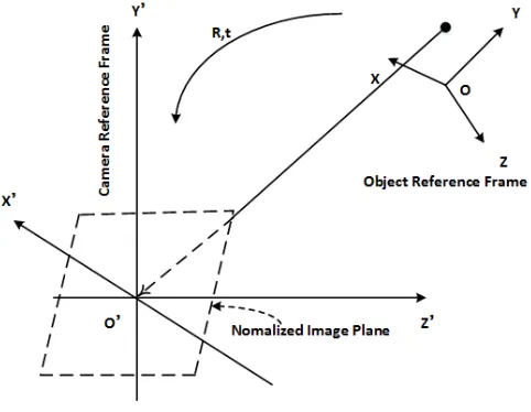
Camera pose estimation is also known as the Perspective-n-Point(PnP) problem. The aim of the PnP problem is to estimate the pose of a calibrated camera and also determine the orientation and position (see Fig. 1). The PnP problem was first proposed in 1981 [6].

Figure 1. The schematic diagram of pose estimation problem.

For non-iterative methods, the pose computational complexity varies between 2 ( )

O n and 8

( )

O n [9]. The

computational complexity of the earlier non-iterative methods is high. In many state-of-the-art methods, the lowest computational complexity is O n( ) (n≥6) [10], but it has been shown unstable for noisy 2D locations and its pose estimation accuracy remains lower than iterative algorithms.

The non-iterative algorithms with computational complexity of O n( ) mainly include: Direct Least Square (DLS) [11], OPnP (n≥3) [12], Direct Linear Transformation (DLT) (n≥6) [13], EPnP (n≥4) [14], A Robust PnP (RPnP) (n≥4) [15]. Due to the first two algorithms have definite objective function, and use algebraic multi-equations to solve this problem, thus the calculation accuracy is high. The last three algorithms have high calculation speed, but generally can not get high calculation accuracy.

The calculation accuracy of iterative methods obviously high. Due to seek one certain solution, generally we need more than 3 points [16]. Most iterative approaches are based on minimizing an error function developed from some nonlinear geometric constraints [17].

The most classical approaches rely on a Gauss-Newton style method and use the projection error as the criterion [18, 19]. Note that, most iterative methods are not robust if own a bad initialization, and suffer from low convergence speed. In POSIT algorithm [20], the position and pose of the camera with the scale of the linear calculation is repeated, POSIT algorithm also take a strategy for calculating the position and the proportion of factors associated with depth. The gOp [21] algorithm and PPnP [22] algorithm are both used as iterative methods to minimize the image-space error function. For gOp, the author uses semi-definite programming (SDP) to estimate the camera pose. However, in PPnP algorithm, in order to establish anisotropic forcing constraint model, the singular value decomposition (SVD) is used.

In particular, Lu [23] introduced a very accurate algorithm, the Orthogonal Iterative (OI) algorithm which is fast in comparison with other iterative ones but slow compared to non-iterative methods. OI algorithm has been widely accepted in real applications, such as in [24], a variant of OI algorithm is proposed for applying it in spacecraft docking [24].

As all we know, facing with the need of real-time calculation situations, in addition to the accuracy requirements, the calculation time is also required [25, 26].

In this paper, we introduce an improved orthogonal iterative algorithm based on the original orthogonal iterative algorithm, the key idea is to integrate the steps in each iteration, our method does not need to solve an absolute orientation problem in every iteration step. The repetitive computation in each iteration can be abstracted and done before iteration. Although the computational complexity of all processes before iterate is O n( ),the computational complexity of each iteration is reduced from O n( ) to O(1). Hence, more iteration can be done in a short time, and the accuracy is improved as well.

An Improved Orthogonal Iterative Algorithm

The Original Orthogonal Iterative Algorithm (OI)

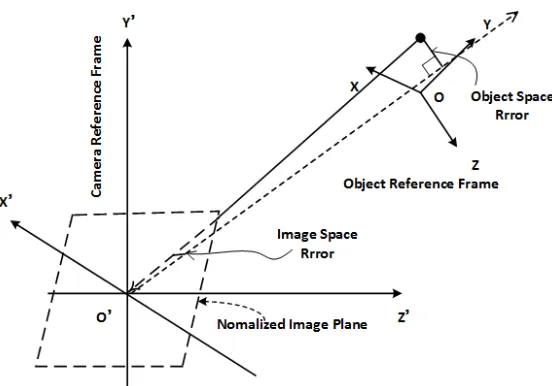
Figure 2. Object-space and image-space collinearity errors.

The sum of the squared error is:

2

1 ˆ

( , ) ( )( )

n

i i i

E R t I V Rp t

=

=

∑

In formula (1),I is identity matrix, p_i is a set of non-collinear 3D coordinates of reference points. We should try our best to minimize this error function over rotation matrix Rand translation vector

t .Noting that, all the information contained in the set of the observed image points { }vi is now

completely encoded in the set of projection matrices vˆ_i.vˆ_i is the observed line-of-sight projection matrix defined as: ˆ _{ˆ ˆ / (ˆ ˆ}T ₎

i i i i

V =v v v v .Since this objective function is quadratic in t , so given a fixed rotationR,the optimal value for t can be computed in closed form as:

1

1 1

1 1 _{ˆ ˆ}

( ) ( )

n n

i i i

i i

t R I V V I Rp

n n

−

= =

 

= _ − _ −



∑

∑

Firstly, assume that the k th estimate of R is k

R , as well, ( ) ( ) ( )

k k

t =t R ,and k k k

i i

q =R p +t .Next

estimation, (k 1)

R + is determined by solving the following absolute orientation problem:

2 1

1 arg min

n

k k

i i R

i

R + Rp t o

=

=

∑

Where the set of k ˆ k i i i

o =V q is treated as a hypothesis of the set of the scene points k i

q . According to

formula (2), we can compute the next translation, as_t( )k _{t R(} (k+1)₎

= .

An Accurate and Accelerative Improvement

In order to facilitate subsequent deduction, we introduce a matrix calculation formula:

( ) ( T ) ( )

Where⊗is Kronecker product,vec( )⋅ refers to the column vector of one certain matrix. Then, Zero-mean value of the reference(base) points can be derived aspi ←pi−p,wherepmeans the mean value of all reference points. Based on formulas (2) and(4).If r=vec R( ),We can infer that:t=G3 9×r. Meanwhile,

1 1

1 1 1 1

1 1 _{ˆ ˆ} 1 1 _{ˆ ˆ}

[ ( )]

n n n n

T T

j j j j j

j j j j

G I V p V I I V p V

n n n n

− −

= = = =

   

=  −  ⊗ − =  −  ⊗



∑

∑

∑

∑

Integrating the projection points: _ˆ ( ) _{ˆ ˆ ˆ}

( ) ( )

k k k k k k k

i i i i i i i i

o =V q =V R p +t = p ⊗V +V G r =J r .In order to use the optimal solution of absolute orientation, the matrix is calculated in each iteration.

1 1 1

( )

n _k n n

k k T k T k T

i i i i i i

i i i

M o o p o p j r p

= = =

=

∑

∑

∑

9 9 1

( )

n

k k k

i i i

m p J r B_× r

=

=

∑

Where the ok is the mean value of all projected points at kth iteration, _mk _{=vec M}( k)_{.According to the}

optimal solution of absolute orientation, the singular value decomposition is k T

M =UDV . In formula (8), updating rotation matrixR in the orthogonal iterative algorithm.

1

k T

R + =UV (8)

we can solve matrix B by using formula (9), meanwhile, the matrix B is a constant matrix during the iteration process.

1 1 1 1

1 1 1 1

ˆ ˆ ˆ ˆ

( ) ( ) ( ) ( )

ˆ ˆ ˆ ˆ

( ) ( )(1 ) ( ) ( )( )

n n n n

T T

i i i i i i i i i i i

i i i i

n n n n

T T

i i i i i i i i i i

i i i i

B p J p p V V G p p V p V G

p p V p V G p p V p V G

= = = =

= = = =

   

= ⊗ = _ ⊗ ⊗ + _= ⊗ ⊗ + _ ⊗ _

= ⊗ ⊗ + ⊗ ⊗ = ⊗ ⊗ + ⊗

∑

∑

∑

∑

∑

∑

∑

∑

In the iteration process, only need to save the matrix B.we can use formulas (7) and (8) to iterative calculate matrixB,finally at the end of the iteration process, we can calculate R, then, based on

3 9

t=G r× , we can calculate t conveniently.

In the same way, for our objective function in formula (1):

2 2

9 9

1 1

ˆ ˆ

( , ) ( )( ) ( )( )

n n

T T

i i i i

i i

E R t I V Rp t I V p I G r r C_×r

= =

=

∑

∑

Where

1

ˆ

( )( )( )

n

T T

i i i

i

C p I G I V p I G

=

=

∑

MatrixCcan also be calculated at the beginning of the iteration process, in the iteration process, the matrix C remains unchanged. The computational complexity of the objective function isO(1).

computational complexity of each iteration is O(1), the computation of the iterative process can be greatly reduced. After the iteration, its easy to calculate the translation vectort.At the same time, its pointed out that, all the computational complexities of formula (5), (9) and (11) are the same O n( ).

Simulation Results

In this section, we compare the other state-of-the-art PnP problem solution methods include: DLT+GN, OPnP, EPnP, OI, against our algorithm, denoted as OI+ algorithm, through computer simulations.

We produce synthetic 3D-to-2D correspondences in a 640×480 image and the virtual perspective camera having an effective focal length f_u = f_v =800pixels. The principle point is (u v_c, _c)=(320, 240). The 3D reference points are randomly distributed in thex−, y−andz− range of [-2,2] × [-2,2] × [4,8].At the same time, we add different levels of Gaussian noise to the points which are on the images.

We define the position and rotation error metrics as:

(12)

The termination condition for both algorithms is that the object space error is less than 6 10−

or there is no improving of the errors between two adjacent iteration steps. All the plots discussed in this section were created by running 1000 independent MATLAB simulations

Where k true

r and_rk_{arekth column of} true

R and R. We run all algorithms in MATLAB 2014a on a PC with 2.2GHz CPU and 6GB RAM.

4 5 6 7 8 9 1011121314151617181920 0

0.5 1 1.5 2

Mean Rotation Error

Number of Points

R o ta ti o n E rr o r (d e g re e s ) DLT+GN OPnP EPnP OI OI+

4 5 6 7 8 9 1011121314151617181920 0

0.5 1 1.5 2

Median Rotation Error

Number of Points

R o ta ti o n E rr o r (d e g re e s ) DLT+GN OPnP EPnP OI OI+

4 5 6 7 8 9 1011121314151617181920 0

0.5 1 1.5 2

Mean Translation Error

Number of Points

T ra n s la ti o n E rr o r (% ) DLT+GN OPnP EPnP OI OI+

4 5 6 7 8 9 1011121314151617181920 0

0.5 1 1.5 2

Median Translation Error

Number of Points

T ra n s la ti o n E rr o r (% ) DLT+GN OPnP EPnP OI OI+

0.5 1 1.5 2 2.5 3 3.5 4 4.5 5 0

50 100 150 200 250 300

Mean Rotation Error

Gaussian Image Noise (pixels)

R

o

ta

ti

o

n

E

rr

o

r

(d

e

g

re

e

s

)

DLT+GN OI EPnP OPnP OI+

0.5 1 1.5 2 2.5 3 3.5 4 4.5 5

0 50 100 150 200 250 300

Median Rotation Error

Gaussian Image Noise (pixels)

R

o

ta

ti

o

n

E

rr

o

r

(d

e

g

re

e

s

)

DLT+GN OI EPnP OPnP OI+

0.5 1 1.5 2 2.5 3 3.5 4 4.5 5

0 50 100 150 200 250 300

Mean Translation Error

Gaussian Image Noise (pixels)

T

ra

n

s

la

ti

o

n

E

rr

o

r

(%

)

DLT+GN OI EPnP OPnP OI+

0.5 1 1.5 2 2.5 3 3.5 4 4.5 5

0 50 100 150 200 250 300

Median Translation Error

Gaussian Image Noise (pixels)

T

ra

n

s

la

ti

o

n

E

rr

o

r

(%

)

DLT+GN OI EPnP OPnP OI+

0.5 1 1.5 2 2.5 3 3.5 4 4.5 5 0 10 20 30 40 50 60 70 80 90 100

Mean Rotation Error

Gaussian Image Noise (pixels)

R o ta ti o n E rr o r (d e g re e s ) DLT+GN OPnP EPnP OI OI+

0.5 1 1.5 2 2.5 3 3.5 4 4.5 5

0 10 20 30 40 50 60 70 80 90 100

Median Rotation Error

Gaussian Image Noise (pixels)

R o ta ti o n E rr o r (d e g re e s ) DLT+GN OPnP EPnP OI OI+

0.5 1 1.5 2 2.5 3 3.5 4 4.5 5

0 10 20 30 40 50 60 70 80 90 100

Mean Translation Error

Gaussian Image Noise (pixels)

T ra n s la ti o n E rr o r (% ) DLT+GN OPnP EPnP OI OI+

0.5 1 1.5 2 2.5 3 3.5 4 4.5 5

0 10 20 30 40 50 60 70 80 90 100

Median Translation Error

Gaussian Image Noise (pixels)

T ra n s la ti o n E rr o r (% ) DLT+GN OPnP EPnP OI OI+

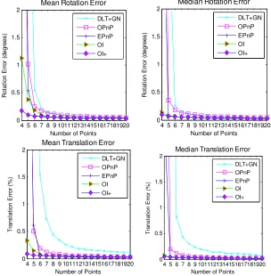
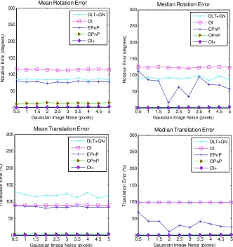
Figure 5. Mean and median errors of rotation and translation with varying noise. (Each point in the plot represents 1000 trials, n=5)

The plots in Figure 3 display the pose as a function of the number of simulation 3D reference points. We first vary the point number n from 4 to 20, adding the same Gaussian noise onto the image,

2

δ= pixels. The number of the independent trials sets at eachnare 1000. Generally, a concise way to summarize the results is to plot both the mean and median errors for all simulations.

From Figure 3 we can observe that our algorithm has definitely better accuracy than the other examined methods we compared with when the point number n is less. It can stably reach the correct result forn≥4 and its accuracy has the high level than the iterative algorithms and other non-iterative algorithms.

As shown in Figure 4 and Figure 5, We change Gaussian noise deviation level δ from 0.5 to 5 pixels, point number fix on n=4 and n=5. we can observe that non-iterative algorithms are not accurate enough and some of them are unstable when n=4,but when n=5,most algorithms can have a high accuracy in different noise. In particular, our OI+ algorithm can have a lowest mean and median error varying the point Gaussian noise, it can be proved that it has a relatively high accuracy and good performance of anti-jamming. But the DLT+GN algorithm is a special one for relatively huge errors, some documents indicate that the DLT+GN is sensitive to noise when the number of reference points is low.

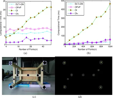
algorithm is not fast enough for real-time applications even with moderate n.In contrast, our OI+ algorithm are faster when n is large, the same with the non-iterative algorithms as OPnP.

4 16 28 40

0 5 10 15 20 25

Number of Points(n)

C

o

m

p

u

ta

ti

o

n

a

l

T

im

e

(

m

s

)

DLT+GN OPnP OI OI+

4 204 404 604 804 1004

0 100 200 300 400 500

Number of Points(n)

C

o

m

p

u

ta

ti

o

n

a

l

T

im

e

(

m

s

)

DLT+GN OPnP OI OI+

(a) (b)

(c) (d)

Figure 6. (a), (b)Average computational time with varying point numbers. (Each point in the plot represents 1000 trials)

(c) Structure of 3D reference control points (d) Reprojection points and the extracted points in real image

Table 1. Results of real experiments.

Algorithms Reprojection object-space error Number of interations Computing times

DLT+GN 0.169 mm 20 6.9 ms

OI 0.156 mm 12 5.6 ms

OPnP 0.147 mm -- 8.8 ms

OI+ 0.124 mm 9 3.4 ms

Real Experiment Results

In order to verify the effectiveness of OI+ algorithm, a set of real experiments is carried out. We design the 3D real reference control points using 9 circle targets, in order to get the accurate world coordinate values, the specific distribution structure is shown in Fig. 6(c).

are shown in Table.1. Reprojection object-space error means the standard deviation of reprojection object-space error at all reference control points. we compare 3 type of algorithms: DLT+GN algorithm, OI algorithm, OPnP algorithm with our OI+ algorithm.

As shown in Table 1, we compare 3 algorithms: DLT+GN, OI,OPnP with our OI+ algorithm and count the reprojection object-space error, number of interations and computing times. Reprojection object-space error means the standard deviation of reprojection object-space error at all reference control points. Our algorithm has a lowest reprojection object-space error in a lowest short time, and it can be proved right and to be effective. Not only the number of interations, but also computing times is lower than other 3 algorithms.

Conclusions

In this paper, aim at classical orthogonal iterative algorithm for camera pose estimation, we proposed an improved accelerated orthogonal iterative algorithm. We integrate the steps in each iteration and the repetitive computation in each iteration can be abstracted and done before iteration. The computational complexity of each iteration is reduced fromO n( )toO(1), thus greatly speeding up the operation of the iterative process. Due to each step complex of our algorithm is constant, so it can adapt more iterations. Meanwhile, to solve the problem of orthogonal iteration local optimal, multiple initial value can be used alone, each iteration, making it easier to find the global optimal solution.

Acknowledgment

This work is supported by The Innovation Fund of Postgraduate, Xihua University (NO: ycjj2016067). The authors also gratefully acknowledge the helpful comments and suggestions of the reviewers, which have improved the presentation.

References

[1] R. Hartley, A. Zisserman, Multiple View Geometry in Computer Vision, Cambridge University Press, Second Edition, 2004.

[2] R. Azuma, Y. Baillot, R. Behringer, et al. Recent advances in augmented reality, Applied Mechanics and Materials, 986-987(2014), 1629-1633.

[3] Z.Y. Zhang, X.H. Huang, J. Yin, et al. Videogrammetric Techniques for Wind Tunnel Testing and Applications, IEEE Computer Graphics and Applications, 21(6), 2011, 34-47.

[4] Li X.D., Guo W., Li M.T, A closed-form solution for estimating the accuracy of depth camera relative pose, Robot, (2), 2014, 194-202, 209.

[5] R. Penne, J. Veraart, & W. Abbeloos, Four point algorithm for recovery of the pose of a one-dimensional camera with un known focal length, Computer Vision, 6(4), 2012, 314-323.

[6] M.A. Fishler, R.C. Bolles. Random sample consensus: a paradigm for model fitting with applications to image analysis and automated cartography, Communications of the ACM, 24(6), 1981,381~395.

[7] L. Kneip, D. Scaramuzza, and R. Siegwart. A novel parametrization of the perspective-three-point problem for adirect computation. Proc. CVPR, 2011, 2969–2976.

[8] L. Quan, Z. Lan, Linear N-point camera pose determination, IEEE Transactions on Pattern Analysis and Machine Intelligence, 21(8), 1999, 774-780.

[10] V. Lepetit, F.M. Noguer, P Fua. EPnP: An accurate O(n) solution to the PnP problem, International Journal of Computer Vision, 81(2), 2009, 155-166.

[11] J.A. Hesch, S.I. Roumeliotis, A Direct Least-Squares (DLS) method for PnP, IEEE International Conf. on Computer Vision, 2011, 383-390.

[12] Y. Zheng, Y. Kuang, S. Sugimoto, et al. Revisiting the PnP problem: A fast, general and optimal solution, IEEE International Conf. on Computer Vision, 2013, 2344-2351.

[13] D. RueB, A., Luber, K. Manthey & R. Reulke, Accuracy evaluation of stereo camera systems with generic camera mod els, International Archives of the Photogrammetry, Remote Sensing and Spatial Information Sciences, B5, 2012, 1124-1135.

[14] I. Zambrano, J. Mez, A. Aguirre Renormalization method and unbiased statistical estimators: an alternative implementation to the EPnP algorithm., CIMAT, 2008.

[15] S.Q. Li, C. Xu, M. Xie. A robust O(n) solution to the perspective-n-point problem, IEEE Transactions on Pattern Analy sis and Machine Intelligence, 34(7), 2012, 1444-1450.

[16] X.S. Gao, X.R. Hou, H.F. Cheng, Complete solution classification for the perspective-three-point problem, IEEE Transations on Pattern Analysis and Machine Intelligence, 25(8), 2003, 930-943.

[17] L. Kneip, D. Scaramuzza, R. Siegwart, A novel parametrization of the perspective- three- point problem for a direct computation of absolute camera position and orientation, The 24th IEEE Conf. on Computer Vision and Pattern Recognition, 2011,2969-2976.

[18] D. G. Lowe, Three-dimensional object recognition from single two-dimensional image, Artificial Intelligence, 31,1987, 355~395,

[19] H. Araujo, R. Carceroni, & C. Brown, A fully projective formulation for Lowe's tracking algorithm, Technical Report 641, Univ. of Rochester, 1996.

[20] S.J. Li, X.P. Liu, An accurate and fast algorithm for camera pose estimation, Journal of Image and Graphics,19(1), 2014, 20-27.

[21] G. Schweighofer, A. Pinz, Globally optimal O(n) solution to the PnP problem for general camera models, British Ma chine vision Conf., 2008, 1-10.

[22] V. Garro, F. Crosilla, A. Fusiello, Solving the P nP problem with anisotropic orthogonal procrustes analysis, Conf. of 3D Imaging, Modeling, Processing, Visualization and Transmission, 2012, 262-269. [23] C.P. Lu, G.D. Hager, E. Mjolsness, Fast and globally convergent pose estimation from video images, IEEE Transactions on Pattern Analysis and Machine Intelligence, 22(6), 2000, 610-622.

[24] S. Zhang, F. Liu, X. Cao, and L. He. Monocular vision-based two-stage iterative algorithm for relative position and atti tude estimation of docking spacecraft, Chinese Journal of Aeronautics, 23, 2010,204~210,

[25] E. Ask, Y. Kuang, & K. Astrom. Exploiting p-fold symmetries for faster polynomial equation solving. Proc. ICPR, 2012.3232–3235.

[26] I. Skrypnyk, D. Lowe, Scene modelling, recognition and tracking with invariant image features, Proceedings of the 3rd IEEE/ACM International Symposium on Mixed and Augmented Reality, 2004, 119.