Volume 2010, Article ID 761460,16pages doi:10.1155/2010/761460
Research Article
A Two-Stage Bayesian Network Method for 3D Human Pose
Estimation from Monocular Image Sequences
Yuan-Kai Wang and Kuang-You Cheng
Department of Electrical Engineering, Fu Jen Catholic University, 24205, Taipei County, Taiwan
Correspondence should be addressed to Yuan-Kai Wang,[email protected]
Received 30 November 2009; Accepted 5 March 2010
Academic Editor: Hsu-Yung Cheng
Copyright © 2010 Y.-K. Wang and K.-Y. Cheng. This is an open access article distributed under the Creative Commons Attribution License, which permits unrestricted use, distribution, and reproduction in any medium, provided the original work is properly cited.
This paper proposes a novel human motion capture method that locates human body joint position and reconstructs the human pose in 3D space from monocular images. We propose a two-stage framework including 2D and 3D probabilistic graphical models which can solve the occlusion problem for the estimation of human joint positions. The 2D and 3D models adopt directed acyclic structure to avoid error propagation of inference. Image observations corresponding to shape and appearance features of humans are considered as evidence for the inference of 2D joint positions in the 2D model. Both the 2D and 3D models utilize the Expectation Maximization algorithm to learn prior distributions of the models. An annealed Gibbs sampling method is proposed for the two-stage method to inference the maximum posteriori distributions of joint positions. The annealing process can efficiently explore the mode of distributions and find solutions in high-dimensional space. Experiments are conducted on the HumanEva dataset with image sequences of walking motion, which has challenges of occlusion and loss of image observations. Experimental results show that the proposed two-stage approach can efficiently estimate more accurate human poses.
1. Introduction
Human pose reconstruction, also called human motion capture, is one of the most popular research topics in com-puter vision and machine learning. Reconstructing human poses can be used to analyze and recognize human behav-iors in many image understanding applications, including human-computer interaction, human-robot interaction, and visual surveillance. Traditionally, motion capture systems use (electro-magnetic or color blob) markers attached to human body to obtain human poses. However, it is uncomfortable and restricts human’s freedom to move. In addition, high cost and obtrusion are two major drawbacks of these systems. Recently, researchers focus on markerless approach which adopts computer vision to analyze human 2D or 3D human poses according to the observations from images [1]. It has the potentiality to provide an inexpensive, non-obtrusive solution and non-restrictive user environment for the estimation of human poses. The complexity of 3D human pose estimation is higher than that of 2D human
pose estimation, because 3D human poses constitute a high-dimensional search space for the computation. Some papers utilize multiple cameras to reconstruct 3D human poses due to that depth information can be obtained
to ease the problem. However,reconstructing 3D human
poses from monocular image sequences is more attractive because it has many advantages such as convenient to use, less restrictions and no computational loading of camera calibration. The challenge of this approach is to infer 3D poses of a highly articulated, self-occluding human gesture from 2D motion sequences without depth information.
It is an ill-posed problem because different 3D human
poses can have the same 2D projection in the image space due to the occlusion problem of human body such as hidden hands and lower limbs occluded by other body parts.
Model-free (or discriminative) and model-based (or generative) methods are two kinds of approaches for
mark-erless monocular human motion capture. Different from
model-based method provides more exact estimation result
of human pose details. Bayesian network is one of effi
-cient ways in model-based approaches. Bayesian network approach can model the kinematics of body configura-tion with probabilistic graphical networks. It constitutes a function mapping from features in images to 3D poses of human body. The estimation of 3D poses is achieved by inferencing posteriori distribution of human body parts from belief propagation in the probabilistic graphical net-works. Although Bayesian network may solve the occlusion problem, an efficient inference algorithm has to be discov-ered.
Previous works inference 3D human poses from monoc-ular image sequences directly by image observations. How-ever, human motions with high-degree freedom usually cause self-occlusion and unpredictability. The function mapping from image observations to 3D poses is highly complex.
Rather than the classical algorithms, in this paper, the function mapping is decomposed into two stages. The two-stage model includes a 2D pose and a 3D pose belief propagation networks. The first stage will estimate 2D poses from image observations, and the second stage reconstructs 3D poses from the estimated 2D results. The adding of 2D human pose information can decompose the indirect causal relationship between image observations and 3D human poses. More accurate inference results can be obtained by reducing the computational complexity of the 3D pose estimation problem. Especially, an annealed Gibbs sampling method is proposed for the inference of the two-stage model. The inference algorithm adopts an annealing process for the sampling of posteriori distributions and can efficiently reconstruct 3D poses. The proposed algorithm has lower cost in computing time than that of Gibbs sampling methods.
Figure 1sketches the proposed two-stage pose estima-tion method. The method includes three important steps that are feature extraction, 2D pose estimation, and 3D pose estimation. The feature extraction step obtains image observations, such as silhouette and appearance features of human. The 2D pose estimation step inferences 2D human poses via these image observations by an annealed Gibbs sampling algorithm. The result of 2D pose estimation step is used to be the observations of the 3D pose estimation step. Both the 2D and 3D models are trained by the Expectation Maximization (EM) algorithm before estimation process. The training features in 2D model training block are the visual features obtained by the feature extraction block. The training features adopted in the 3D model training block include 2D inference results and parts of visual features that can provide 3D information.
The remainder of this paper is structured as follows.
Section 2 reviews earlier related work. Our approach is presented in Sections3and4. InSection 3, a formal descrip-tion of the proposed two-stage probabilistic framework is presented. This is followed inSection 4by the extraction of image observations of the human poses. Experimental results are reported inSection 5to discuss the performance of the approach.Section 6concludes the paper.
2. Review of Previous Work
Model-free approach [2–7] is one kind of monocular
pose estimation approach that establishes a direct relation between image observation and human motion. It recovers the kinematics configuration of a person whose appearance in images varies due to different clothing and lighting condi-tions. This approach exploits model variations in pose con-figuration, human shape, and appearance, without assuming
human body model. Agarwal and Triggs [8] proposed an
algorithm to estimate 3D human model from silhouette of single view using nonlinear regression to model the relation between histograms of shape contexts and human pose. They [9] also used histograms of gradient orientations over a grid of small cells with nonnegative matrix factorization to gain a set of basis vectors corresponding to local features of body parts. Bowden et al. [10] extracted 2D silhouette of a moving human and the corresponding 3D skeletal structure to be image observations and adopted a non-linear point distribution model (PDM) to fit them. Silhouette is a good feature to help recover 3D poses since it is insensitive to the variations in color and texture [9]. Rohr [11] used edge lines to replace edges in order to partially get rid of silhouette noise. Although all these model-free methods provide interesting results, the robustness of these methods will suffer since articulated relationship of human body parts is not incorporated to solve the occlusion problem.
The goal of model-based approach is to construct the function that gives the likelihood of the image, given a set of parameters which include body configuration parameters, body shape and appearances. The approach usually adopts an articulated model to represent the relationship among human body parts as a kinematics tree, consisting of divisions linking by joints. The prior knowledge describing kinematic properties by shape, texture and appearance has been used to make the problem tractable. One of the fundamental representations is the Johansson’s moving light displays [12]. It adopted a relatively simple representation of the human body called the stick figure that consists of line segments linked by joints. It was demonstrated that relatively little information (motion of a set of selected points on the body) is needed for humans to perform reconstruction of the body configurations. Pose estimation is challenging due to its non-rigid nature, self-occlusion, variable appearance, and high degree of freedom. By incorporating articulation knowledge, model-based approaches are able to overcome these problems to a great extent and are actively explored by many researchers.
EM training
EM training
Testing image
2D model training
Result
3D model training
2D Bayesian inference with annealed Gibbs
sampling
3D Bayesian inference with annealed Gibbs
sampling
Training
features
Training
features 3D Bayesian
human model setting
2D Bayesian human model
setting
Feature extraction
Figure1: Flowchart of the proposed method.
using Nonparametric Belief Propagation and particle filters. Hua et al. [15] exploited a data driven belief propagation Monte Carlo algorithm with importance sampling functions building from bottom-up visual cues for efficient inference. Using Markov network has the advantage that every node would influence their neighbors and converges to a stable result. However, errors may be easily propagated to all nodes in the network.
In Bayesian network models, nodes have directed arcs linked to other nodes, which are also called a directed acyclic graph (DAG). These arcs represent the relation of cause and effect between nodes. Parent nodes in DAG are not influenced by their child nodes. Human body parts with stable movement, such as torso, are usually considered to be the root node and/or parent node. Child nodes represent the body parts with high freedom of movement that have large location variations and can also represent image features [16–18]. Leonid and Darrell [19] used a generative appearance model defined by Bayesian networks. The Bayesian generative appearance model is similar to [20] for 3D articulated tracking and [21] for modeling the interactions of multiple independent moving objects. Compared with Markov networks, Bayesian network is more efficient when there are stable visual features assistant for the finding of body parts. Another advantage is that estimation errors of specific body objects would not propagate to other body elements.
Previous works of belief propagation approach pay atten-tion on one-stage framework, which estimates 3D human poses directly from image observations. However, obtaining 3D body pose from visual features can be considered as a machine learning problem that approximates a function
mapping of a given data space to targeted pose space. This function seems to be highly complex. Since same visual features can represent different body pose configurations and same body configurations can generate different visual features due to clothing and view-point, it makes the
ill-posed problem more difficult. Therefore, the search of
posterior distributions in high-dimensional state space from sparse learning data is still intractable. Motivated partly by these issues, a two-stage framework with an annealed Gibbs sampling inference algorithm which can increase estimation accuracy and reduce computation time is proposed in this paper.
3. The Two-Stage Framework for
Pose Estimation
This section will give a two-stage Bayesian network frame-work including 2D and 3D articulated human models for the estimation of human poses. The proposed Bayesian network is a belief propagation network using an annealed Gibbs sampling algorithm to estimate 2D and 3D human joint positions.
Left shoulder
Left elbow
Left hand
Left knee
Left foot
Neck
Left
waist Right
waist Right shoulder
Bottom
Right hand Right
knee
Right foot
Right elbow
x
y
z
(a)
Head
Left shoulder
Left elbow
Left hand
Left knee
Left foot
Neck
Left waist
Right waist
Right shoulder
Bottom
Right hand Right
knee
Right foot
Right elbow
(b)
(c) (d)
Figure2: Articulated human model. (a) 3D model and joints, (b) 2D model and joints, (c) projected model on the image, (d) joint positions
mapping to the human body.
Directed graph is used for the abstraction of the artic-ulated human models. The human pose is defined as a node setH = {H2D,H3D}, whereH2D = {h2d,1,. . .,h2d,15}, H3D = {h3d,1,. . .,h3d,15}, andh2d,i andh3d,iare the 2D and
3D positions of the ith joint. Shown in Figures 3(a) and
3(b)are the graphical model of humans. According to the directed graphical model, each node is affected only by its parent node.
The representation of 2D and 3D poses is a probabilistic stick figure with joint positions but not joint angles. The disadvantage of joint angle representation is that more body parameters such as limb length and global orientation of
body have to be given for pose estimation. On the other hand, joint position can uniquely encode the pose of human.
A Bayesian network is a directed acyclic graph −→G = (V,−→E,C) defined by a set of nodesV, a set of directed edges −
→
E, and an edge cost function C defined as C : (i,j) →
h2d,6 h2d,4 h2d,2 h2d,1 h2d,3 h2d,5 h2d,7 h2d,15
h2d,9 h2d,8 h2d,10
h2d,12 h2d,11
h2d,14 h2d,13
(a)
h3d,15
h3d,1 h3d,2 h3d,3
h3d,4 h3d,5
h3d,8 h3d,6
h3d,9
h3d,12 h3d,10
h3d,7
h3d,11
h3d,14 h3d,13
(b)
Figure 3: Graphical model. (a) 2D graphical model, (b) 3D
graphical model.
given an instantiation of its parents. In other words, for each nodeViwith parentsVj ∈ pa(Vi), an edge (i,j) exists and
there is a conditional probability distribution P(Vi | Vj)
representing the edge cost function for the edge; for each Viwithout parents, there is a prior probability distribution
P(Vi).
We denote our 2D and 3D Bayesian networks as −
→
G2D = (V2D,−→E2D,C2D) and −→G3D = (V3D,−→E3D,C3D), where V2D = {H2D,O2D} and V3D = {H3D,O3D} are two sets of random variables describing the joints and observations of human body parts. The 2D observation set O2D = {fk, 1 ≤ k ≤ n} consists of the visual features:
contour point set, normalized center, spatial distribution
h3d,i
WN L
S Nc
h2d,i
C
SDS (a)
h3d,i
WN L
S Nc
C
SDS (b)
Figure 4: Comparison of one-stage and two-stage networks for
pose estimation. (a) The proposed hierarchy of causal relationship among observations, 2D poses, and 3D poses, (b) one-stage network directly linking observations and 3D poses.
of skin color, and corners, which will be discussed in
Section 4. The 3D observation setO3D= {O3d,1,. . .,O3d,15} is defined by O3d,j = {h2d,j,wN,L} includes not only
some visual features, but also the corresponding 2D joint positions of the body parts h2d,j as the observations. The
directed edges−→E2D= {(h2d,i,h2d,j), (h2d,i,O2D)}and−→E3D =
{(h3d,i,h3d,j), (h3d,i,O3d,i)}can be categorized into two edge
sets. The edges (h2d,i,h2d,j) and (h3d,i,h3d,j) link joint nodes
and are illustrated in Figure 3. The edges (h2d,i,O2D) and (h3d,i,O3d,i) link joint nodes and observation nodes and
are illustrated in Figure 4(a). It is the proposed two-stage hierarchy which is different with usual one-stage networks shown in Figure 4(b). The edge cost functions of 2D and 3D models, C2D = {P(h2d,i | pa(h2d,i)} and C3D =
{P(h3d,i | pa(h3d,i)}, are conditional distributions obtained
by EM learning algorithm. The proposed two-stage hierarchy decomposes the direct function mapping of visual features to 3D poses into two steps: first mapping visual features to 2D poses, and then mapping 2D poses and visual features to 3D poses. The method can increase accuracy since the exploration space in each stage is smaller than that in the direct function mapping.
The proposed DAG encodes the cause-effect and
The proposed network structures specify two unique
joint probability distributions (JPD) P2D(V2D) and
P3D(V3D). They will be simply denoted as P(V) in the following derivations since both distributions have the same Markov property.P(V) reflects the properties of the network and can be factorized into the product of all conditional probability distributions
P(V)=
n
i=1
PVi|pa(Vi)
, (1)
where n is the number of all nodes in the network.
This factorization of the JPD comes from a local Markov
property called Markov blanket [22]. Namely that each
variable is independent of its nondescendents in the graph given the state of its parents. Theconditional independence property can reduce, sometimes significantly, the number of parameters that are required to characterize the JPD of the variables. This reduction provides an efficient way to compute the posterior probabilities given the evidence.
There are two problems for the computation of human posesH: the parameter learning of the conditional distri-butions P(Vi | pa(Vi)), and the inference of the posterior
probabilities ofHgiven the evidence O,P(H | O). Details will be given in next two subsections.
3.2. Parameter Estimation by EM Algorithm. Learning pro-cess is important for Bayesian network. The training data consisting of human poses and observations is incomplete and sparse. The learning algorithm of Bayesian network has to be built on a high-dimensional solution space and solve the local maxima problem. In this paper, we use the EM algorithm [23] to train the 2D and 3D graphical models.
In the proposed Bayesian network, the local
probabil-ity distribution for each node is formulated by P(Vi |
pa(Vi),θ,Sh),whereθis the parameter vector of probability
distribution, and Sh is the topology of the 2D or 3D
Bayesian network. Parameter learning is used to find a good approximation parameterθforθ that can be explained by the training data setD= {D1,. . .,DN}, whereNrepresents
the number of training samples.Dl = {V1[l],. . .,Vn[l]}is
thelth training sample. A log-likelihood functionLD(θ) =
log(P(D | θ)) is formulated based on the independence
assumption of training samples and can be decomposed into the product of all conditional distributions according to the conditional independence property:
LD(θ)=log ⎧ ⎨ ⎩ N
l=1
P(V1[l],. . .,Vn[l]|θ) ⎫ ⎬ ⎭ = n
i=1
N
l=1
logPVi[l]|pai(Vi(l)),θ
.
(2)
We obtain the parameter θby the Maximum Likelihood
Estimation (MLE) method:θ=arg maxθLD(θ)0.
However, the training data Dis incomplete because of self-occlusion of body parts. That is, the variablesVi[l] or
parents of the variableVj[l] ∈ pa(Vi[l]) in (2) are hidden
and missing. The partial observability induces the so-called incomplete data problem. Hence, MLE can not be directly utilized for the training. The EM algorithm is a common method solving the learning of incomplete data.
Assume D is incomplete. We can claim D = Y ∪U,
whereY is an observed data set and Uis the missing data set. The EM learning algorithm guesses a probable initial θ(0) at the start of learning process, and then proceeds to repeatedly generate θ(t) iteratively by Expectation-step and Maximization-step.
The Expectation-step computes the conditional expecta-tion of the log likelihood funcexpecta-tion with a givenY and the current parameterθ(t):
Qθ|θ(t)=Eθ(t)=
logP(D|θ)|θ(t),Y. (3)
The Maximization-step updates thet+ 1 step parameter θ(t+1)from current parameterθtunder the assumption that
the Expectation-step computes a correctθt:
θ(t+1)=arg max
θ Q
θ|θ(t). (4)
The Expectation-step and Maximization-step are repeated until the difference ofLD(θ(t+1))−LD(θ(t)) converges.
3.3. Posterior Inference by Annealed Gibbs Sampling. Esti-mating human poses given a set of observations can be formulated as a probabilistic inference problem. Let the
observed data be O = O −U, where U is the set of
hidden variables that are unobservable due to occlusion. The best estimated pose is a vectorH∗, which is defined as the pose with the maximum probability givenO. The posterior probabilityP(H | O) is maximized over all possible pose space according to Bayes’ rule and marginalization as follows:
H∗=arg maxP(H|O)
=arg max
u∈UP(H,u|O
)du
=arg max
u∈U P(H,O
,u)du,
(5)
with the assumption that the prior distribution P(H) is
uniform. The functionP(H,O,u) is a specific case of the full JPDP(V) becauseV=H∪O∪U. Substituting (1) into (5) we obtain the inference formulation:
H∗=arg max
u∈U
i=1,...,n
PVi|pa(Vi)
du. (6)
The direct way for the full integration over continuous variables is called exact inference that can obtain precise inference results when querying the Bayesian network. Although the high-dimensional JPD is factored into the product of low-dimensional conditionals, it still takes high computational complexity and known to be an NP-hard problem. Some algorithms, such as junction tree and mes-sage passing algorithms, can efficiently inferenceH∗only in restricted classes of networks.
Approximate inference methods [24] have also been
proposed in the literature, such as the loopy belief prop-agation, variational methods, and Markov chain Monte Carlo (MCMC) sampling methods. Approximate inference
methods have low computational complexity. MCMC [25]
is attractive because it solves the integration problem in high-dimensional space by gradually improving estimates as sampling proceeds. A variety of standard MCMC methods, including the Metropolis-Hastings algorithm and the Gibbs sampling, were used for approximate inference.
The MCMC sampling methods obtain samples of the target distributionP(V) by Markov chain. A sample vectorv is defined as a sample of the random vectorV. Attiteration, a candidate vector v∗ is sampled from v(t−1), the sample
vector of V obtained at t −1 iteration, and a proposal
distribution q(v∗ | v(t−1)). The candidate is accepted as the new state v(t) with a probability α(v(t−1),v∗) =
min(1,p(v∗)q(v(t−1) | v∗)/ p(v(t−1))q(v∗ | v(t−1))). This generates a Markov chain (v(0),v(1),. . .,v(k),. . .), as the tran-sition probabilities fromv(t−1)tov(t)depends only onv(t−1) and not (v(0),v(1),. . .,v(t−2)). Following a sufficient burn-in period (of, say,ksteps), the chain approaches its stationary distribution and samples from the vector (v(k+1),. . .,v(k+n))
are samples from P(V). The Monte Carlo integration
method can then be applied to solve (5). However, the
sampling of P(V) is still not efficient if V is in a high-dimensional space.
In this paper, a Gibbs sampling method with annealing process is proposed for the inference of the Bayesian network. The key to the annealed Gibbs (AG) sampler is that we only consider univariate conditional distributions sampled with a stochastic process controlled by simulated cooling process. The AG sampler is first proposed by S. Geman and D. Geman [26] for Markov random fields with Gibbs field. Here the sampler is revised for the proposed two-stage Bayesian network.
We define an expression of full conditionals asP(Vj |
V−j)=P(Vj|V1,. . .,Vj−1,Vj+1,. . .,Vn) whereV−jdenotes
a vector containing all of the variables butVj. It follows by
the Markov blanket property [25] that the full conditionals
can be simplified as follows: P(Vj | V−j) = P(Vj |
pa(Vj))
k∈ch(Vj)P(Vk | pa(Vk)), where ch(Vj) denotes the
children nodes of Vj. That is, we only need to take into
account the parents, the children, and the children’s parents. Sampling from the full conditionals, with the AG sampler, lends itself naturally to the construction of general purpose MCMC.
We define the samples ofVj, thejth variable ofV, asvj.
The samplesvjare drawn from the distributionP(Vj|V−j).
Thus, to obtain thev(jt), that is,vjin thetth iteration of the
sampling process, we draw from the distribution
v(jt)∼P
Vj|v1(t),. . .,v (t)
j−1,v (t)
j+1,. . .,v(nt)
. (7)
Therefore, the AG sampler adopts the proposal distribution forj=1,. . .,n
qv∗|v(t)= ⎧ ⎪ ⎨ ⎪ ⎩
pv∗j |v(−i)j
ifv∗−j=v−(t)j
0 otherwise. (8)
If the probability of the move for v(jt) is α(v( t)
j ,v∗) =
min(1,p(v∗)q(v(jt)|v∗)/ p(v
(t)
j )q(v∗|v
(t)
j ))=1, it becomes
a Gibbs sampler. However, the AG sampler is proposed to improve the iteration process. It is similar to Metropolis sampling but has different probabilityαof a move given by
αAG=min ⎛ ⎜ ⎝1,
⎛ ⎝ p(v∗)
pv(jt)
⎞ ⎠
1/T(t)
qv(jt)|v∗
qv∗|v(t)
j
⎞ ⎟ ⎠. (9)
The idea is that when we initially start sampling the space, we will accept a reasonable probability of a down-hill move in order to explore the entire space. As the process proceeds, we decrease the probability of such down-hill moves. Function T(t) is called cooling schedule and the particular value ofT at any point in the chain is called the temperature. Typically, T0is start time andTf is the final cool down temperatures
over nstep. A typical setting of geometric decline for the temperature is given by
T(t)=T0
Tf
T0 t/n
. (10)
The AG sampler adopts a stochastic iterative algorithm that converges to the set of points which are the global maxima of the given function. The annealing process can find the maximum of complex distributions with multiple peaks where standard hill-climbing approaches may trap the algorithm at a less optimal peak.
The advantage of the AG sampler is its efficiency com-pared to the Gibbs sampler. Instead of wanting to approx-imateP(V), we want to find the global maximum, that is, the ML estimate of posterior distribution. We could run a Markov chain of invariant distributionP(V) and estimate the global mode byH∗ =arg maxV(t),i=1,...,N
u∈U P(V(t))du.
However, this method is inefficient because the random
samples only rarely come from the vicinity of the mode. Unless the distribution has large probability mass around the mode, computing resources will be wasted exploring areas of no interest.
This annealing process involves simulating a non-homogeneous Markov chain whose invariant distribution at iteration t is no longer equal to P(V), but to Pt(V) ∝
P1/T(t)(V), where lim
t→ ∞T(t)=0. The reason for doing this
(a)
(b) (c)
Figure5: Human silhouette. (a) Original image, (b) extracted contour of the human, (c) uniformly sampled points of the extracted contour.
0 50 100 150 200 250 300 350 400 450
Pix
el
ac
cum
ulation
value
0 100 200 300 400 500 600
xcoordinate of image
Normalized width
(a)
Length Normalized width
(b)
(a) (b)
(c)
0 10 20 30
1 2
3 4
5 1
2 3
4 5
(d)
Figure7: Spatial distribution of skin color. (a) Skin color detection, (b) noise removal and pixel grouping by morphology, (c) region
segment, (d) the spatial distribution of skin color in (c).
Figure8: Corners of silhouette.
4. Feature Extraction
Image features, such as edge, color, and silhouette, are observations of a pose. The extraction of image features constitutes evidence nodes of the articulated human model for the inference in the Bayesian network. Single human feature is not enough to inference 3D human position since different 3D poses can exhibit similar 2D observations in the images. Therefore, we devise 4 kinds of features in the proposed method: human silhouette, normalized center of
human body, spatial distribution of skin color, and corners of human body.
4.1. Human Silhouette. Human silhouette is a useful feature with highly resistance to the change of appearance and illu-mination. Silhouette features contain full body information, including head, torso, and limbs.Figure 5(a)is an original
image from HumanEva I database [27, 28]. The subject
image is segmented from background and transformed to a binary image.Figure 5(b) is the contour image extracted by topological structural analysis. The extracted contour is then uniformly sampled into a contour point set, which is depicted inFigure 5(c).
4.2. Normalized Center. Normalized center is proposed to normalize position-dependent features, such as silhouette. However it cannot be readily obtained because human’s shape varies frame by frame due to its nonrigid characteris-tics caused by limbs motion. A normalized widthwN, instead
(a) (b)
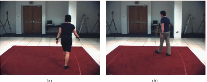
Figure9: Sample images of the walking sequences used in our experiments.
if hx threshold andhx−1 < threshold forx = 1 → w, and xR = x if hx threshold and hx+1 < threshold for x=w → 1. The threshold is determined by empirical study from experimental results.
As we getwN we can obtain the normalized boundary
rectangle shown in Figure 6(b). We calculate the center of normalized boundary rectangle that is called normalized centerNcas shown inFigure 6(b). Assume that the left top
point of normalized boundary rectangle is calledp.We can
define the x and y coordinates of the normalized center
Nc as xN = xp + 0.5wN, yN = yp+ 0.5L, where L is the
boundary length of subject. BothwnandNcwill be used as
the observations in the two-stage Bayesian network.
4.3. Spatial Distribution of Skin Color. Appearance feature which is proposed in this paper is called spatial distribution of skin color. We use the Gaussian Mixture Model (GMM) to obtain skin color regions [29]. The GMM uses multiple Gaussians to model the probability of skin color pixels in the image. EM algorithm is utilized to find the parameters of the GMM. A 2D histogram of the skin color pixels is then computed to describe to the spatial distribution of those skin color pixels.
Figure 7(a) presents extracted skin color regions of
Figure 5(a)by the GMM method. Shown inFigure 7(b)is the result of morphology that is adopted to remove noises and fill in connected components. The minimum bounded area of the subject is then equally divided into several smaller blocks, which are illustrated in Figure 7(c). Accumulated number of skin color pixels in each block is calculated. Figure 7(d)
illustrates the ratio of skin color pixels of each block to total skin color pixels in the image, which is the 2D histogram, describing the spatial distribution of skin colors.
4.4. Corners of Human Body. Corners of human shape have strong relationship to joints of body parts. It can be exploited by Bayesian networks as good observations for the finding of 2D human body parts. We use the level curve curvature method [30] that defines corners as areas. These areas have level curves multiplied by the gradient magnitude raised to the power of 3 which can intensify the level curves and help
the search of local maximum.Figure 8shows the extracted corners.
The four visual features complement each other. The silhouette feature can well describe the localization of human shape, but is prone to occlusion. Normalized center is helpful for estimating proximal and distal joints of torso. Never-theless, simply using the feature is not appropriate because the high-degree freedom of limbs influences the boundary’s width. Skin color distribution is the feature sensitive to the change of illumination, but offers good indications of the positions of face and limbs. Corners potentially indicate joint locations of human. The locations of knees and feet that we are interested in have high probability close to corners of human silhouette, because they are joints of human.
5. Experimental Results
5.1. Experimental Setup. The proposed method has been evaluated to demonstrate its effectiveness. Experiments are carried out to compare the proposed method with the Gibbs sampling method. The method is implemented with C and C++, and experiments are conducted on a PC with 2.4 GHz Pentium 4 CPU and 1 GB memory.
We presents experimental results conducted on the image sequences in the HumanEva dataset [27,28]. It is a dataset including both video and ground-truth 3D motion captured by multiple cameras and a calibrated marker-based motion capture system. The image sequences are captured with a resolution of 644×488 pixels and a frame rate of 120 Hz. Human activities in the dataset are played by multiple subjects performing a set of predefined actions with a number of repetitions. The dataset has been divided into separate training and testing sets.
The motion capture data given by the HumanEva dataset will be used to train our model and test as ground truth data. The motion capture data provides 3D position information about the location of a set of markers roughly corresponding to a subset of major human body joints. 3D marker positions are projected into 2D marker positions by perspective geometry.
GT AGs
(a)
GT AGs
(b)
GT AGs
(c)
GT AGs
(d)
GT AGs
(e)
GT AGs
(f)
GT AGs
(g)
GT AGs
(h)
Figure10: Results of estimated 2D pose projected onto images. Green dotted lines are the ground truth and yellow lines represent estimation
result of our method. (a)–(d) Subject 1. (e)–(h) Subject 2.
three times at the edge of the capture space. The walking sequences contain a full 180◦turn that induces the challenges of occlusion of body parts and loss of visual features.
Some example images are shown in Figure 9. Note that
to demonstrate the method’s ability of occlusion handling with monocular images, only the image sequences from single camera are adopted for the experiments. No depth information is utilized. Also, other image sequences such as running and jogging are not tested in our experiments because fast-motion gestures are only critical to tracking
problems which is not the concern of this work. The Bayesian network proposed in this paper is used to the detection of reconstructed poses.
−50 0 50 100 150
100 0
−100 0 −100
−50 0 50 100 150
100 0
−100 0 −100
Ground truth AGs estimation result
(a)
−50 0 50 100 150
100 0
−100 −100 0
100 −50 0 50 100 150
100 0
−100 0
100 −100
Ground truth AGs estimation result
(b)
−50 0 50 100 150
100
0 −100
0 −100
100 −50 0 50 100 150
100 0
−100
0 100 −100
Ground truth AGs estimation result
(c)
−50 0 50 100 150
100 0
−100
0 −100
100 −50 0 50 100 150
100 0
−100
0
100 −100
Ground truth AGs estimation result
(d)
−50 0 50 100 150
100 0
−100
0 −100
100 −50 0 50 100 150
100 0
−100
0
100 −100
Ground truth AGs estimation result
(e)
−50 0 50 100 150
100 0
−100
0 −100
100 −50 0 50 100 150
100 0
−100
0
100 −100
Ground truth AGs estimation result
(f)
−50 0 50 100 150
100 0
−100
0 −100
100 −50
0 50 100 150
100 0
−100
0
100 −100
Ground truth AGs estimation result
(g)
−50 0 50 100 150
100 0
−100
0 −100
100 −50
0 50 100 150
100 0
−100 0
100 −100
Ground truth AGs estimation result
(h)
Figure11: Results of estimation result in 3D space. (a)–(h) The left figures are ground truth, and the estimated results are shown in the right
0 50 100 150 200 250
ξ
(mm)
GS AGS
Algorithms One-stage
Two stage
(a)
0 10 20 30 40 50
A
ver
age
computing
time
(s)
GS AGS
Algorithms One-stage
Two stage
(b)
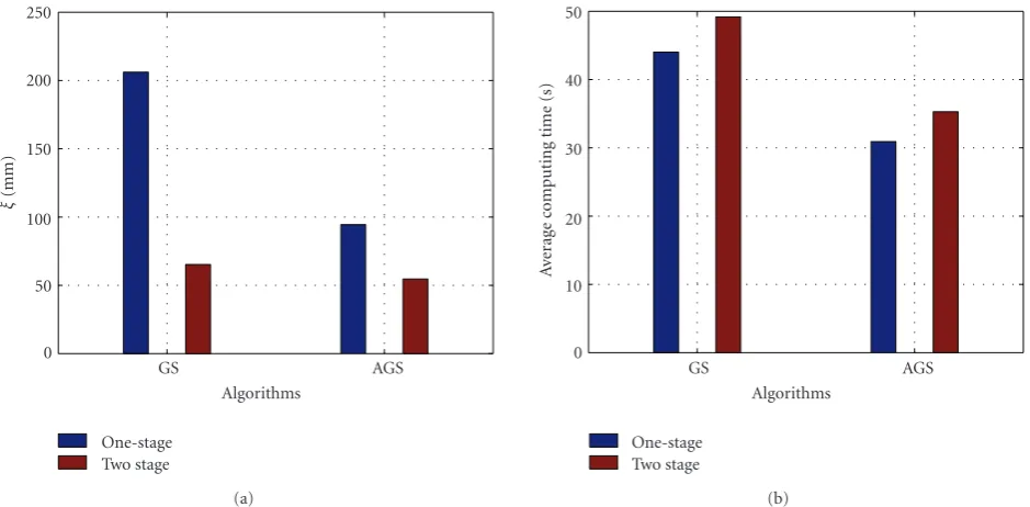
Figure12: Performance comparison between the two-stage and one-stage methods. Both the Gibbs sampling and the annealed Gibbs
sampling algorithms are implemented for the two methods. (a) Average distance errors, (b) average computing time.
40 45 50 55 60 65 70 75 80 85 90
ξ
(mm)
20 25 30 35 40 45 50
Iterations Gibbs
Annealed Gibbs
Figure13: The effect of iteration number on accuracy.
can estimate joint parts that are out of our vision because they are occluded by other body parts. Some local errors, mostly due to the lack of visual features and occluded parts, can be observed. For example, the local error of left arm in
Figure 10(a)is produced because the left arm is occluded by torso. The head positions are sometimes less accurate when skin area of face becomes invisible. However, the estimates are still fairly consistent among these results.
Figure 11presents the estimation results of 3D human structure in 3D space. Our method can simulate the hidden body part to solve the occlusion problem and reconstruct the human pose approximately. On this challenging set of images, the overall 3D pose estimation is fairly satisfactory. It
has to be noticed that no tracking algorithm is incorporated in our method. The presented results are obtained frame by frame from monocular images. The local errors can be alleviated by further exploiting pose tracking from multiple cameras, or introducing more accurate feature descriptor.
To quantitatively examine the performance of the pro-posed method, a measurement is defined by a distance error of poses between estimated results and ground truth. SupposeH = {h1,h2,. . .,hM}, wherehm ∈R3(orxm ∈R2
for the 2D body model), is the position vector of the body pose in the world (or image, resp.). The error in estimated poseH∗to the ground truth poseHcan then be expressed as the average absolute distance between individual body parts,
D(H,H∗)=
M
m=1
hm−h∗
m
M . (11)
ForN sequences ofT frames we can compute the average
distance error using the following:
ξ= 1 NT
N
n=1
T
t=1
DHt,n,Ht∗,n
. (12)
30 35 40 45 50 55 60 65 70 75 80
ξ
(mm)
10 12 14 16 18
Burn-in Gibbs
Annealed Gibbs (a)
3 3.5
4 4.5
5 5.5
6 6.5
7 7.5
8
ξ
(pix
el)
10 12 14 16 18
Burn-in Gibbs
Annealed Gibbs (b)
Figure14: Average distance errors of the proposed two-stage method with respect to different burn-in numbers. (a) 3D distance errors, (b)
2D distance errors.
attribute this largely to that the sampler only explores the mode of the likelihood function, but not the entire likelihood space. Finally, the annealed two-stage method can achieve the best performance.
Algorithmic comparison was evaluated with the Bayesian framework of sequential importance resampling and annealed particle filtering, which is the baseline algorithm provided in the HumanEva for evaluation and comparison. An average distance error of 68 mm was obtained. Compared to the 51 mm average distance error of the proposed method, the annealed two-stage method can get better performance.
The behaviors of the two-stage method with respect to the iteration number and burn-in parameters were investigated.Figure 13shows the effect of changing iteration parameter from 10 to 50. We observe that increased iteration number reduces distance errors. The decrease of distance errors converges at the 40 iterations. Different values of burn-in were also tested.Figure 14shows the average distance error of 3D and 2D poses with respect to the burn-in periods with 40 iterations. In general, the performance of the proposed two-stage method is not sensitive to burn-in values. The errors for both Gibbs sampler and the AG sampler are fairly stabilized for 3D and 2D estimations. However, in all these burn-in parameters the estimation of AG sampler is consistently more accurate than that of Gibbs sampler.
6. Conclusions
We have presented a novel approach to solve the problem of 3D pose estimation from monocular image sequences. The approach proposes a two-stage inference hierarchy of Bayesian network. Visual features are extracted as the observations in the first stage of the network for the inference of 2D poses. The 2D poses along with assisted visual features are then applied for the inference of 3D poses. The EM algorithm is applied for the learning of network parameters.
The advantages of the two-stage approach are twofold: First, it can improve the accuracy of 3D poses estimation; Second, both 2D and 3D poses are obtained by the same computational framework.
We introduce the use of simulated annealing as an
effective mechanism to improve inferences. An annealed
Gibbs sampler has been proposed for the inference of the two-stage Bayesian network. The sampler adopts an annealing process to explore the proposal distribution of sampling. The exploration can concentrate on the mode of the distribution and achieve more efficient computation. Experimental results demonstrate that the annealed two-stage approach has better accuracy and efficiency than one-stage method.
The approach currently has two limitations, first, the technique needs more accurate visual features to help the exploration of inferences. Second, temporal and spatial information are not incorporated into the approach to pre-dict and smooth the inference result of each frame. Tracking algorithm and multiple cameras can further improve the estimation.
References
[1] R. Poppe, “Vision-based human motion analysis: an over-view,”Computer Vision and Image Understanding, vol. 108, no. 1-2, pp. 4–18, 2007.
[2] M. Brand, “Shadow puppetry,” in Proceedings of the IEEE International Conference on Computer Vision (ICCV ’99), vol. 2, pp. 1237–1244, Kerkyyra, Greece, September 1999. [3] A. Elgammal and C.-S. Lee, “Inferring 3d body pose from
silhouettes using activity manifold learning,” in Proceedings of the IEEE Computer Society Conference on Computer Vision and Pattern Recognition (CVPR ’04), vol. 2, pp. 681–688, Washington, DC, USA, June 2004.
sequences,” in Proceedings of the European Conference on Computer Vision, vol. 3024 of Lecture Notes in Computer Science, pp. 442–455, Prague, Czech Republic, 2004.
[5] R. Rosales and S. Sclaroff, “Inferring body pose without tracking body parts,” in Proceedings of the IEEE Computer Society Conference on Computer Vision and Pattern Recognition (CVPR ’00), vol. 2, pp. 721–727, Hilton Head Island, SC, USA, June 2000.
[6] E.-J. Ong and S. Gong, “A dynamic 3D human model using hybrid 2D-3D representations in hierarchical pca space,” in Proceedings of the British Machine Vision Conference, pp. 33– 42, Nottingham, UK, 1999.
[7] C. J. Taylor, “Reconstruction of articulated objects from point correspondences in a single uncalibrated image,” Computer Vision and Image Understanding, vol. 80, no. 3, pp. 349–363, 2000.
[8] A. Agarwal and B. Triggs, “A local basis representation for estimating human pose from cluttered images,” inProceedings of the 7th Asian Conference on Computer Vision, Part I (ACCV ’06), vol. 3851 ofLecture Notes in Computer Science, pp. 50–59, Hyderabad, India, January 2006.
[9] A. Agarwal and B. Triggs, “Recovering 3D human pose from monocular images,”IEEE Transactions on Pattern Analysis and Machine Intelligence, vol. 28, no. 1, pp. 44–58, 2006.
[10] R. Bowden, T. A. Mitchell, and M. Sarhadi, “Non-linear statistical models for the 3D reconstruction of human pose and motion from monocular image sequences,” Image and Vision Computing, vol. 18, no. 9, pp. 729–737, 2000.
[11] K. Rohr, “Towards model-based recognition of human move-ments in image sequences,” Computer Vision, Graphics and Image Proceeding: Image Understanding, vol. 59, no. 1, pp. 94– 115, 1994.
[12] G. Johansson, “Visual perception of biological motion and a model for its analysis,”Perception and Psychophysics, vol. 14, no. 2, pp. 201–211, 1973.
[13] L. Sigal, S. Bhatia, S. Roth, M. J. Black, and M. Isard, “Tracking loose-limbed people,” in Proceedings of the IEEE Computer Society Conference on Computer Vision and Pattern Recognition, vol. 1, pp. 421–428, Washington, DC, USA, June 2004.
[14] S.-F. Lan, M.-F. Ho, and C.-L. Huang, “Human motion parameter capturing using particle filter and nonparametric belief propagation,” inProceedings of IEEE Southwest Sympo-sium on Image Analysis and Interpretation, pp. 37–40, Santa Fe, NM, USA, 2008.
[15] G. Hua, M.-H. Yang, and Y. Wu, “Learning to estimate human pose with data driven belief propagation,” inProceedings of the IEEE Computer Society Conference on Computer Vision and Pattern Recognition (CVPR ’05), vol. 2, pp. 747–754, San Diego, Calif, USA, June 2005.
[16] D. Ramanan, D. A. Forsyth, and A. Zisserman, “Tracking people by their appearence,” IEEE Transactions on Pattern Analysis and Machine Intelligence, vol. 29, pp. 65–80, 2007. [17] M. W. Lee and I. Cohen, “A model-based approach for
esti-mating human 3D poses in static images,”IEEE Transactions on Pattern Analysis and Machine Intelligence, vol. 28, no. 6, pp. 905–916, 2006.
[18] N. Thome, D. Merad, and S. Miguet, “Human body part labeling and tracking using graph matching theory,” in Pro-ceedings of IEEE International Conference on Video and Signal Based Surveillance (AVSS ’06), pp. 38–46, Sydney, Australia, November 2006.
[19] T. Leonid and T. Darrell, “Bayesian articulated tracking using single frame pose sampling,” inProceedings of International Workshop on Statistical and Computational Theories of Vision, Nice, France, 2003.
[20] N. Jojic, M. Turk, and T. S. Huang, “Tracking self-occluding articulated objects in dense display maps,” inProceedings of International Conference on Computer Vision, pp. 123–130, Kerkyra, Greece, 1999.
[21] N. Jojic and B. J. Frey, “Learning flexible sprites in video layers,” inProceedings of the IEEE Computer Society Conference on Computer Vision and Pattern Recognition, vol. 1, pp. 199– 206, Kauai, Hawaii, USA, December 2001.
[22] M. I. Jordan,Learning in Graphical Models, The MIT Press, Cambridge, Mass, USA, 1998.
[23] T. K. Moon, “The expectation-maximization algorithm,”IEEE Signal Processing Magazine, vol. 13, no. 6, pp. 47–60, 1996. [24] C. Borgelt and R. Kruse,Graphical Models: Methods for Data
Analysis and Mining, Wiley, Chichester, UK, 2002.
[25] C. Andrieu, N. De Freitas, A. Doucet, and M. I. Jordan, “An introduction to MCMC for machine learning,”Machine Learning, vol. 50, no. 1-2, pp. 5–43, 2003.
[26] S. Geman and D. Geman, “Stochastic relaxation, Gibbs distributions, and the Bayesian restoration of images,”IEEE Transactions on Pattern Analysis and Machine Intelligence, vol. 6, no. 6, pp. 721–741, 1984.
[27] A. O. Bˇalan, L. Sigal, and M. J. Black, “A quantitative evalua-tion of video-based 3D person tracking,” inProceedings of the 2nd Joint IEEE International Workshop on Visual Surveillance and Performance Evaluation of Tracking and Surveillance (VS-PETS ’05), pp. 349–356, Beijing, China, October 2005. [28] L. Sigal and M. Black, “HumanEva: synchronized video and
motion capture dataset for evaluation of articulated human motion,” Tech. Rep. CS-06-08, Brown University, 2006. [29] L. M. Bergasa, M. Mazo, A. Gardel, M. A. Sotelo, and L.
Boquete, “Unsupervised and adaptive Gaussian skin-color model,”Image and Vision Computing, vol. 18, no. 12, pp. 987– 1003, 2000.