PERFORMANCE ANALYSIS OF WLAN UNDER VARIABLE NUMBER OF NODES USING THE ADJUSTABLE PARAMETERS IN EDCA

(1)

ISSN: 1992-8645 www.jatit.org E-ISSN: 1817-3195

ADAPTIVE NONLINEAR CONTROL OF THREE-PHASE

SHUNT ACTIVE POWER FILTERS: POWER FACTOR

CORRECTION AND DC BUS VOLTAGE REGULATION

1_{A. AIT CHIHAB,}2 _{H. OUADI,}3_{F. GIRI}

1,2_{PMMAT Lab, Department of Physics, Faculty of Science, University Hassan II, Casablanca (Morocco).} 3

GREYC Lab, UMR CNRS 6072, University of Caen Basse-Normandie (France). E-mail: [email protected], [email protected] ,[email protected]

ABSTRACT

The problem of controlling three-phase shunt active power filters (SAPF) is addressed in presence of nonlinear loads supplied with three-phase power grids. The SAPF-load system is shown to be modeled, in the (, ) coordinate frame, by a third-order nonlinear state-space representation. The control objective is twofold: (i) compensating for the current harmonics and the reactive power absorbed by the nonlinear load; (ii) regulating the inverter DC capacitor voltage. To this end, a nonlinear adaptive controller is developed on the basis, on the average system model, using the backstepping design technique. The controller is made adaptive for compensating the uncertainty on the unknown SAPF components and on the switching loss power. The performances of the proposed adaptive controller are formally analyzed using tools from the Lyapunov stability and the averaging theory. The theoretical results are confirmed by numerical simulations.

Keywords: Active Power Filters, Current Harmonics, Reactive Power, Backstepping, Lyapunov Stability,

Average Analysis.

1. INTRODUCTION

Power grids and distribution networks are expected to simultaneously interact with a wide variety of loads. The latter range from single AC motors (e.g. in electrical traction) to much more complex plants involving several types of machines and power electronics equipments organized in smaller size subgrids. As a matter of fact, these loads (whatever their size), such as rectifiers, power supplies and speed drivers, involve nonlinear dynamics that entail the generation of current harmonics and the consumption of reactive power. If not appropriately compensated for, the current harmonics and the reactive power are likely to cause several harmful effects e.g. the distortion of the voltage waveform at the point of common coupling (PCC), and the overheating of transformers and distribution lines. Moreover, the disturbing effect of current harmonics may go beyond the PCC reaching other loads and electronic equipments connected to the net, causing boosted ageing of those loads and making harder the synchronization with the network voltage in applications requiring such synchronization.

(2)

The complexity of SAPF power systems control lies in the fact that the above control objectives must be carried out despite the system dynamics nonlinearity and the system model parameter uncertainty. A great deal of interest has been paid to this control problem over the last decade. However, most available solutions are limited to the simpler case of mono-phase SAPFs, e.g. [1], [2], [3], [4]. The point is that mono-phase SAPFs are only useful in low power applications. The problem of controlling three-phase SAPF power systems has been dealt with following three approaches. The first consists in using hysteresis operators or fuzzy logics [5],[6]. These methods do not make use of the exact nonlinear SAPF model in the control design. Consequently, the obtained controllers are generally not backed by formal stability analysis and their performances are generally illustrated by simulations. The second control approach consists in using linear controllers (e.g. [7], [8], [9]). With linear controllers, optimal performances can not be guaranteed on a wide range variation of the operation point, due to the nonlinear nature of the controlled system dynamics. The third approach consists in using nonlinear controllers designed on the basis of the system accurate nonlinear models. The used control design techniques include passivity approach e.g. [10], Lyapunov design e.g [11] and sliding mode control [12]. However, the proposed nonlinear controllers have only consisted in current loops designed to meet the current harmonic compensation requirement. Without an explicit voltage regulation loop, the DC voltage regulation objective cannot be achieved in presence of wide disturbance (e.g fugitive large load variation). Besides, the previously proposed nonlinear controllers are designed assuming all SAPF parameters to be perfectly known and the switching losses in the inverter to be negligible. The point is that some SAPF parameters are quite ill known (e.g. Decoupling filter resistor , leak resistance ). Also, the switching losses can hardly be ignored as they act on the DC bus voltage.

In this paper, the focus is made on the control of energy systems that involve three-phase SAPFs and nonlinear loads. A new control strategy is developed that simultaneously meets the PFC requirement i.e. on one hand, well compensation of current harmonics and the reactive currents absorbed by the nonlinear three-phase load and, on the other hand, a tight regulation of the inverter DC capacitor voltage. To this end, an adaptive cascade nonlinear controller is developed using the backstepping and other Lyapunov-like techniques.

The controller inner loop involves a current regulator designed to cope with harmonics compensation. The outer-loop involves a voltage regulator that maintain the DC line voltage at its possibly varying reference values. The controller is provided with adaptation capability making it able to cope with the uncertainty on the (possibly varying) switching losses in the inverter. Interestingly, the controller involves a current harmonics estimator, designed by the instantaneous power technique, making possible online tuning of the inner loop reference signal. A second contribution of this work consists in designing a parameter estimator making possible the determination of the time-invariant unknown parameters Rf and Rdc. It is formally shown, using

tools from the Lyapunov stability and the averaging theory, that all control objectives are actually achieved in the mean. This theoretical result is confirmed by several numerical simulations illustrating additional controller robustness features. The paper is organized as follows: the control problem formulation, including the SAPF modeling, is described in Section 2; The time-invariant uncertain parameters estimations; the adaptive nonlinear cascade controller design and performance analysis are presented in section 3; the theoretical performances are confirmed by simulation in Section 4, A conclusion and a references list end the paper.

2. MODELING OF THREE-PHASES SAPF

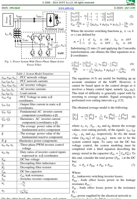
The three-phase SAPF under study has the structure of Fig 1. It consists of a three-phase full-bridge inverter and an energy storage capacitor , placed at the DC side. From the AC side, the SAPF is connected to the network through a filtering inductor (, ); this reduces the circulation of the harmonics currents generated by inverter switching. The SAPF function is to produce reactive and harmonic components to neutralize the undesirable current harmonics produced by the nonlinear load. The DC-AC inverter operates in accordance to the well-known pulse width modulation principle (PWM), [13], [14].

The notations of TABLE 1 are used in the description of the system model.

Applying the usual electric laws to the three-phase shunt APF one easily gets:

(3)

On the other hand, the output voltages and output currents of the DC-AC inverter are given by the following expressions e.g. [13]:

೏೎

2 1 1 1 2 1 1 1 2

(2)

(3)

Where the inverter switching functions (i =a, b

or c) are defined by:

௜ 1 ₁௜ଵ ; ௜ଶ ௜ଵ ; ௜ଶ

Substituting (2) into (3) and applying the Concordia transformation, one obtains the filter equations in α

-β coordinates:

೑

(4)

(5)

The equations (4-5) are useful for building up an accurate simulator of the SAPF. However, it cannot be based upon in the control design as it involves a binary control input, namely , . This kind of difficulty is generally coped with by resorting to average models. Signal averaging is performed over cutting intervals e.g, [13].

The obtained average model is the following:

(6)

where , , , and denote the average values, over cutting periods, of the signals , , , and , respectively. In (6), the mean value , of , turns out to be the system control input. To carry out the DC bus voltage control, the system modeling must be completed with a third equation describing the energy stored in the capacitor (

). To this end, consider the total power () at the DC bus:

(7)

Where:

, (unknown) switching inverter losses;

, Joule effect losses power in the leakage resistance ;

, Joule effect losses power in the resistance ;

, power supplied by the electrical network to maintain in charge the DC bus capacitor. It is readily checked that:

Table 1. System Model Notations

, , : PCC network voltage , , : PCC network currents , , : AC inverter voltages. , , : AC inverter currents. , , : Load current.

, : PCC Voltage in static α-β coordinates.

, : Output filter current in static α-β coordinates.

, : Fundamental AC inverter current component (coordinates α-β) , : Harmonics AC inverter current

component (coordinates α-β) : The average power value of the

fundamental active component : The average power value of the fundamental reactive component , ! :Harmonics power components , , : Three-phase PWM inverter control

voltage

, : Duty ratios of inverter control inputs expressed in α-β coordinates

: DC bus voltage

: Decoupling filter inductance : Decoupling filter resistor : DC bus capacitor.

"

: leak resistance.

: Switches inverter components

# :

Nonlinear load.

,

R L

P

o

w

er

n

et

w

o

rk

,

[image:3.612.85.527.56.697.2]

SAPF

(4)

$ %

(8)

(9) $ %

(10) &' (11)

Where denotes the instantaneous energy in the capacitor.

Let denote the averaged capacitor energy. Then, one gets introducing (8)-(11) in (7):

೏೎మ

ವ಴ (12)

Using (1), equation (12) simplifies to:

ଷ ௙ఈ௙ఈ ௙ఉ ௙ఉ

௏೏೎ మ

ோವ಴ ௦௖

(13)

Using (2), one gets by operating the usual averaging (over cutting periods) on all signals in

(13):

ଷ

௏೏೎ మ

ଶ ఈ௙ఈ ఉ ௙ఉ

௏೏೎ మ

ோವ಴ ௦௖ (14)

For convenience, the model equations (6) and (14) are rewritten altogether:

#

(

(15) )

# (16)

The system (15)-(16) is clearly nonlinear

3. THREE-PHASE SAPF ADAPTIVE

CONTROLLER DESIGN

The adaptive controller design in this section is composed of two main components: an adaptive observer and a cascade regulator.

3.1 Adaptive observer design

Some parameters of the SAPF model (15)-(16) are subject to uncertainty, this is the case of the decoupling filter resistor , the capacitor leakage resistance and the decoupling filter inductance whose value may be subject to uncertainty, following the magnetic saturation. In this section, we present a parameter identifier that determines accurate estimates of these unknown parameters, based on the available signal

measurements i.e. output filter current , and DC bus voltage ( ).

From the state filter equations model (15)-(16), the candidate observer is given by

*+ +, #+

(

- +

+ (17) .+ / )

#+ 0 - + (18)

With + (k=1, 2, 3); #+ (i=1, 2) and - (i=1, 2) are respectively the state estimation, the parameter estimation and the observer gain

Subtracting the SAPF model (15)-(16) and the observer model (17)-(18), one obtains:

*! !, #!

-!

! (19) .!/ #! -! (20)

With ! (k=1, 2, 3) and #! (i=1, 2) are respectively the state and parameter error estimation.

In order to ensure the convergence to zero of the estimation errors, let us introduce the following Lyapunov candidate function:

ଵ

ଵ ଶଵ

ଶଵ ଶଶ

ଶଵ ଶଷ

ଶ ଵ

ଶఊభଵ

ଶ ଵ

ଶఊమଶ

ଶ ଵ

ଶఊయ௦௖

ଶ

(21)

The time derivative of the candidate Lyapunov function is given by:

!! !! !! #!#!

#!#!

(22)

Substituting (19)-(20) into (22) we get:

-! -! -! #!&

#! !

!' #!

#! !

! (23)

3.2 Cascade regulator design

3.2.1 Control objective reformulation

(5)

objectives and to design the controller. Presently, the decomposition is performed using the so-called instantaneous power technique, which enjoys a good compromise between accuracy and computational complexity [15].

Accordingly, the active and the reactive load powers can both be decomposed, when the load currents include harmonics, in a continuous component and a varying component, i.e.

!

(24)

Solving the equation (24) with respect to the currents, and rearranging terms, one gets the following decomposition:

∆

0

23333433335 !"

_∆_23333433335 ₀ # !"

∆

!

23333433335

$ #! !" (25)

With ∆

Control objectives. We seek the achievement of the two following control objectives:

−−−− Controlling the filter current (and ) so that the load current harmonics and the load reactive currents are well compensated for. −−−− Regulating the DC bus voltage () to maintain

the capacitor charge at a suitable level so that the filter operates properly.

One difficulty with the problem at hand is that, there are three variables that need to be controlled (i.e. , and ), while one has only two control inputs (i.e. and ). This is coped with by considering a cascade control strategy involving two loops (Fig. 2). The outer control loop aims at regulating the DC bus voltage. The control signals generated by the outer loop regulator, denoted (,), serve as the desired fundamental

components of the output current filter. These components are augmented with the (load current) harmonic and reactive components, next denoted ∗ , ∗ ), to constitute the final AC current references ∗and ∗ . Accordingly, one gets the following reference signals:

∗ ∗

∆

!

23333433335 $ #! !"

_∆_23333433335 ₀ # !" ₇

& !"

(26)

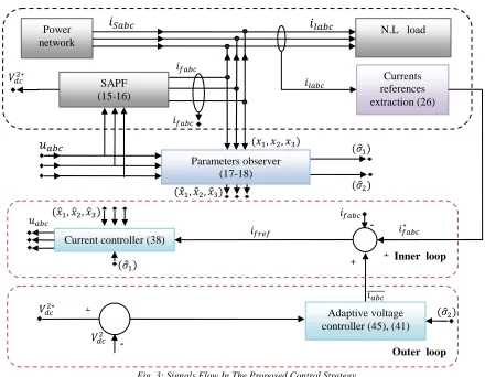
The signal flow involved in the proposed control strategy is illustrated by Fig. 2.

3.2.2. Cascade regulator design:

Inner loop. This is designed to make the current

tracking errors,

8 + ∗ 8 + ∗

as small as possible. To this end, the dynamics of these errors needs to be determined. It follows, using estimator model equation (17), that the errors undergo the following equations:

8

8 #+

(

- + +

∗

∗ (27) To ensure the asymptotic stability of the equilibrium8, 8 0,0, consider the Lyapunov candidate function defined by:

1₂8₈ '

8 8 Deriving along (27) yields:

88 '

;#+

(

- + +

∗

∗< (28) Outer loop. This aims at making the voltage

tracking error,

8 + ∗ (29) as small as possible, where ∗ is the reference value of the DC bus voltage. These together with its first time-derivative are assumed to be known and bounded.

Furthermore, by respecting the notations presented in TABLE 1, the ac filter currents verify:

(30)

(6)

ଷ ௙ఈ ௙ఉ

௙ఈ

௙ఉ

௙ఈ ௙ఉ !௙ఈ

! ௙ఉ ௩೏೎

మ

ோವ಴ ௦௖

(31) On the other hand, in practice state variable present a very slow dynamic (it is associated to the DC bus) then the AC current components ( ) and (). Indeed, the latter are varying at harmonics load current frequency. Consequently, the control design is based on the average model, obtained

form (31) letting there 〈 〉 0 . It turns out that the average DC voltage state is

given by:

(33) Time derivative of the error voltage gives, using (29) and (33):

8 ! ∗ #+ 0 -! ∗ (34) The switching-loss power () is seen as an unknown parameter in (34). Indeed, the latter is mainly depending on the load which presently is assumed to undergo a piecewise constant variation.

On the other hand, the quantity stands in (34) as a virtual control. Interestingly, with (8) and (32) this quantity is nothing other than the electric network power, denoted ,

transmitted to control the voltage DC bus. Indeed, with (8) and using (32) one shows that equals: $ %

(35) In order to obtain a stabilizing control law of the error system (34), (27) and (19)-(20), let us introduce the following full Lyapunov function candidate:

8 (36)

With (23) and (28) deriving along (34), (27) and

(19)-(20), yields:

-! -! -! ₈8 '

;#+

(

- + + ∗

∗< 8 #+ 0 -! ∗

#!&

#! ! !' #!

#! !

! (37) Equation (37) suggests the following control inputs (, ), which defines the inner regulator:

∗, ∗ ,,

∗, ∗

∗ +,,, #+, #+

,

ሺ݅

_!

ሻ

∗

, , ∗, ∗

∗_,

∗ + +

,,

N.L Load Power

grid net

Active

filter

Voltage regulator Current regulator

Currents references construction #+, #+

Inner loop

Outer loop

Fig. 2: Synoptic Scheme Of The Cascade Control Strategy. State variables estimated and adaptive parameters

(7)

) ;#+

- + +

∗ ∗

?8

?8 < (38)

It also suggests the following virtual outer loop control:

?8 #+ 0 -!∗ (39)

Finally, equation (37) suggests the following parameter adaptation law:

#! #+ @! ! (40) #! #+ @! (41)

0 @! (42)

In fact, substituting (38)-(42) in (37) yields:

-! -! -! ?8 ?8 ?8 (43)

Now, as is a virtual control input, we make use of equation (35) to obtain:

)

0 (44) Substituting (39) into (44) one gets the following expression of the fundamental of the current references:

)A

&?8

PC*+ -!

∗_'

&?8

PC*+ -!

∗_'D

(45) The adaptive outer regulator thus designed includes the parameter adaptation law (42) and the control law (45). Its performances are described in the following theorem.

Remark 1. Although the (inner and outer) control laws (38) and (45) involve a division by and , respectively, which entails a risk of singularity. However, this risk is purely theoretical as in practice the active filter cannot work if and are null. In other words, the latter are nonzero as long as the active filter is carrying non-identically null currents.

Theorem: Consider the closed-loop system composed of the SAPF represented by the model (15)-(16) and the adaptive controller consisting of:

- The adaptive state observer described by equations (17)-(18),

- The cascade regulator including the (inner) current control loop defined (38) and (40) and the (outer) voltage control loop (41), (42) and (45). 1) The closed-loop system is described in the error coordinates $! ! ! 8 8 8 #! #!% by the following equations:

*! !, #!

-!

! .!/ #! -!

8 8

?8

?8 8 ?8

#! #+ @! ! #! #+ @! 0 @!

2) The above error system has a stable equilibrium at $! ! ! 8 8 8 #! #!% = $0 0 0 0 0 0 0 0 0% with respect to the Lyapunov function V defined by (36).

3) The current tracking errors 88, the DC voltage tracking error 8, and the states estimation errors !, !, ! all converge to zero.

Proof. Part 1 is readily established putting together equations (19)-(20), 27, 34 and (40)-(42). Part 2 follows from (43) which show that is a semi-definite negative function of the error vector. Part 3 is established applyimg the LaSalle’s invariant set principle. To this end, let E⊂, be the set

where 0. One gets from (43) that E F$0 0 0 0 0 0 G G G%' H ,I. Also, J⊂Z

denotes the largest invariant set of the error system of Part 1. By LaSalle’s invariant set principle, one concludes that $! ! ! 8 8 8 #! #!% converges, whatever its initial conditions, to M. It turns out that $! ! ! 8 8 8 %' is asymptotically vanishing. This completes the proof of the Theorem.

4-SIMULATION AND DISCUSSION OF RESULTS

(8)

[image:8.612.311.529.89.288.2]

Fig. 3: Signals Flow In The Proposed Control Strategy.

Outer loop +, +, +

+ +

݅

_ௌ௔௕௖

, ,

#+

∗

#+

#+ +, +, +

#

∗

ݑ

_௔௕௖

݅

_௟௔௕௖

N.L load Power

network

SAPF (15-16)

Adaptive voltage controller (45), (41) Current controller (38)

Currents references extraction (26)

+

-

Parameters observer (17-18)

Inner loop

-

[image:8.612.85.295.108.250.2]

of the load and the active filter are described by Table 2.

The inner adaptive control law, the outer regulators and the adaptive observer are implemented using equations (38), (45), (40)-(42) and (17-18), respectively. The corresponding design parameters are given the following numerical values of Table 3, which proved to be convenient. In this respect, not that there is no systematic way, especially in nonlinear control, to make suitable choices for

these values. Therefore, the usual practice consists in proceeding with trial-error approach.

Doing so, the numerical values of Table 3 are retained.

The whole simulated control system is illustrated by Fig. 3

Figures 4 and 5 show the shape of the load current (respectively in temporal and frequency domains). It is readily seen that the load current is actually rich in harmonics components

.

Table 2. Shunt Apf Characteristics

PARAMETERS VALUES

Power active filter

Lf Cf Rf

0.022H. 1000 µF. 0.007 Ω. Rectifier-Load L

R

10 mH. 100 Ω

Extraction filter Order 2

Cut frequency 218rd/s

Table 3. Adaptive Controller Parameters

Current regulator

c1 5.103 c2 5.103

Voltage regulator c3 100

Adaptive observer - - @ @ @

[image:8.612.90.530.351.693.2]

(9)

0 200 400 600 800 1000 1200

0 0.5 1 1.5 2 2.5 3

frequency in HZ

lo

a

d

c

u

rr

e

n

t

in

A

Fig.4: Load Current In Time Domain.

Fig.5: Load Current In Frequency Domain.

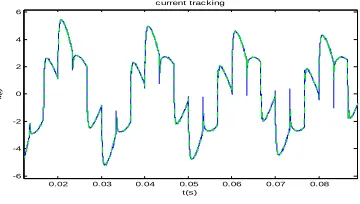
The resulting controller performances are illustrated by Figs. 6 to 8. Figs. 6 shows that the AC three-phases filter currents track well their references, confirming the results of subsection 3.2.2 (equation (38)). The resulting network line current is plotted in Fig. 7 which shows that this current is clearly clean of harmonics, unlike the load current. This is better illustrated by Fig. 8 which shows the spectra of the load and net currents. It is seen that the net current is mainly constituted by a single component, situated in 50Hz. The higher frequency harmonics have well been suppressed

.

[image:9.612.250.516.65.624.2]

The performances of the adaptive observer are showed through the figures 9-11. These figures show that the SAPF states estimated errors converge to zero. The estimation errors parameters are bounded as expected, confirming the theoretical result of subsection 3.

Fig 7. Network Current (௦ఈ) In Time Domain

Fig 8: Network Current(௦ఈ) In Frequency Domain

Fig.9: State Estimation Errorଵ.

[image:9.612.106.286.582.684.2]

Fig.10: State Estimation Error ଶ

Fig.11: State Estimation Error ଷ

To highlight the robustness of the proposed control law, a disturbance is injected (see Fig.12) at the entrance of SAPF representing a fugitive discharge of DC bus capacitor. The perturbation introduced during this validation test appears (see Fig.13) at time 0.12s. Fig.14 shows the good behavior of the DC voltage outer loop.

0.02 0.03 0.04 0.05 0.06 0.07 0.08 0.09 0.1 0.11 -4

-2 0 2 4 6

current tracking

if

(t

)

t(s)

0.5 0.51 0.52 0.53 0.54 0.55 0.56 0.57 0.58 0.59 0.6 -15

-10 -5 0 5 10 15

time in s

n

e

tw

o

rk

c

u

rr

e

n

t

in

A

0 200 400 600 800 1000 1200

0 0.5 1 1.5 2 2.5 3

frequency in HZ

n

e

tw

o

rk

c

u

rr

e

n

t

in

A

0.005 0.010.015 0.020.025 0.030.035 0.040.0450.050.055 -0.2

-0.15 -0.1 -0.05 0 0.05 0.1 0.15 0.2 0.25

estimation error

X

1

(t

)

t(s)

0.005 0.01 0.015 0.02 0.025 0.03 0.035 0.04 0.045 -0.1

-0.05 0 0.05 0.1 0.15

estimation error

X

2

(t

)

t(s)

0.005 0.01 0.015 0.02 0.025 0.03 0.035 0.04 -1

-0.8 -0.6 -0.4 -0.2 0 0.2 0.4 0.6

estimation error of x(3)

X

3

(t

)

t(s)

Fig.6: Output Active Filter (௙ఈ) Current And Its

Reference

0.02 0.03 0.04 0.05 0.06 0.07 0.08

-6 -4 -2 0 2 4 6

current tracking

if

(t

)

(10)

5. CONCLUSION

The problem of controlling three-phase shunt active power filters is addressed in presence of nonlinear loads and uncertainty on the SAPF parameters (Rf, Rdc). The control objective is to achieve, on one

hand, current harmonics and reactive power compensation and, on the other hand, tight voltage regulation at the inverter output capacitor. This control problem is dealt with by designing a nonlinear adaptive controller composed of the adaptive observer (17-18) and a cascade controller consisting of the inner control law (38) and the outer control law (45). It is formally established that the controller meets its objectives. This formal result is confirmed by several simulations which further show the robustness of the proposed control strategy to external tough disturbances.

REFERENCES:

[1] Matas J, L.G.De Vicuna, J.Miret, J.M.Guerrero, and M.Castilla, ''Feedback linearizations of a single-phase active power filter via sliding mode control,'' IEEE Trans. Power Electronics, vol. 23, pp. 116-125, 2008. [2] Etxeberria-Otadui, I., A.L.de Heredia, H.Gaztanaga, S.Bacha, Reyero, M.R ''A single synchronous frame hybrid (SSFH) multifrequency controller for power active filters,'' IEEE Trans. Ind. Appl., vol. 53, no. 5, pp. 1640–1648, 2006.

[3] Komurcugil, H. ''A new control strategy for single-phase shunt active power filters using a Lyapunov function,'' IEEE Trans. on Industrial Electronics, vol. 53, pp. 305 – 312, 2006.

[4] Hurng-liahng Jou, Hui-yung Chu & Jinn-Chang Wu, ''A novel active power filter for reactive power compensation and harmonic suppression,'' International Journal of ElectronicsVolume 75, Issue 3, September 1993, pages 577-587 Published online: 24 Fab 2007.

[5] HAMZA BENTRIA "A shunt active power filter controlled by fuzzy logic controller for current harmonic compensation and power factor improvement" JATIT, 15th October 2011. Vol. 32 No.1

[6] Brahim. BERBAOUI, Chellali.

BENACHAIBA, Rachid.DEHINI,

Brahim.FERDI."Optimization of shunt active power filter system fuzzy logic controller based on ant colony algorithm" JATIT 2010

[7] B.suresh kumar, K.ramesh reddy, Y.lalitha " PI, fuzzy logic controlled shunt active power filter for three-phase four-wire systems with balanced, unbalanced and variable loads " JATIT 2011.

[8] Abdelmadjid Chaoui, Jean Paul Gaubert, Fateh Krim & Gérard Champenois, ''PI Controlled Three-phase Shunt Active Power Filter for Power Quality Improvement'' Journal of Electric Power Components and Systems Volume 35, Issue 12, September 2007, pages 1331-1344, Published online: 19 Sep 2007.

[9] Zanchetta P., M., Sumner, M., Marinelli, F., Cupertino ''Experimental modeling and control design of shunt active power filters'' Control Engineering Practice 17 (2009) 1126–1135, 2009.

[10] Escobar, G., A.M. Stankovic, and P.Mattavelli, (2004)“An adaptive controller in stationary reference frame for D-statcom in unbalance operation,”IEEE Trans. Ind. Electron., vol. 51, no. 2, pp. 401–409.

[11] Rahmani, S., A.Hamadi, and K.Al-Haddad ''A Lyapunov-Function-Based Control for a Three-Phase Shunt Hybrid Active Filter'' IEEE

[image:10.612.96.304.72.443.2]

Fig 13: Injected Perturbation.

Fig 14: Outer-Loop Tracking Performances: Capacitor Energy And Its Reference.

0 0.05 0.1 0.15 0.2 0.25 0.3 0.35 0.4 0.45

0 20 40 60 80 100 120

0 0.05 0.1 0.15 0.2 0.25

0 20 40 60 80 100 120 140 160 180

Voltage Sensor

+

-

∗ ∗

+

-

Voltage controller

Perturbation

Current Controller

+

X

#

PWM

SAPF

(11)

Transactions On Industrial Electronics, Vol. 59, No. 3, pages:1418-1429, 2012.

[12] Ernesto Wiebe, José Luis Durán & Pedro Rafael Acosta,''Integral Sliding-mode Active Filter Control for Harmonic Distortion Compensation'' Journa of Electric Power Components and SystemsVolume 39, Issue 9, May 2011, pages 833-849, Published online: 8 Jun 2011.

[13] Krein P.T., J. Bentsman, R.M. Bass, and B. Lesieutre ''On the use of averaging for analysis of power electronic system,''. IEEE Trans. Power Electronics, vol. 5, pp. 182-190,1990. [14] Tse, C. K. and M. H. L. Chow ''Theoretical

study of switching converters with power factor correction and output regulation,'' IEEE Trans. Circuits & Systems I, vol. 47, pp. 1047–55, 2000.