TEXTURE PATTERN IN ABNORMAL MAMMOGRAMS CLASSIFICATION USING SUPERVISED MACHINE LEARNING TECHNIQUES

4256

EVALUATION AND ANALYSIS OF PID AND FUZZY

CONTROL FOR AUV-YAW CONTROL

1_{MOHD SHAHRIEEL MOHD ARAS,} 2_{BOON PEI TEOW,} 2_{AI KEE TEOH,} 2_{PEI KEE LEE,}

3_{ANUAR MOHAMED KASSIM,} 4_{MOHAMAD HANIFF HARUN,} 5_{MOHD KHAIRI MOHD}

ZAMBRI, 5_{ALIAS KHAMIS}

1,3_{Senior Lecturer, Center for Robotics and Industrial Automation, Faculty of Electrical Engineering,}

Universiti Teknikal Malaysia Melaka (UTeM), MALAYSIA.

2_{Student, Department of Mechatronics, Faculty of Electrical Engineering, Universiti Teknikal Malaysia}

Melaka (UTeM), MALAYSIA.

4,5,6_{Lecturer, Center for Robotics and Industrial Automation, Faculty of Electrical Engineering, Universiti}

Teknikal Malaysia Melaka (UTeM), MALAYSIA . E-mail: 1_{[email protected]}

ABSTRACT

This paper presents the comparison and performances analysis between Proportional Integral Derivative (PID) Controller and Fuzzy Logic Controller (FLC) designs for yaw control of an Autonomous Underwater Vehicles (AUVs). PID controller is easy to be implemented as PID parameter can be obtained based on the software used and it’s can be achieved, precisely. Moreover, the PID parameter can be acquired based on tracking error and treats the system to be “blackbox” if the system parameter is unknown. However, the designed PID controller may not resist the uncertainties and disturbances. Hence, FLC design had been implemented to improve the performances of AUV-yaw control using heuristic approach until the satisfactory results are obtained. It is necessary to tuning the rules and the range of membership functions in order to get the desired output and improve the system response. The aim of this work is to analysis the performances between PID and FLC for AUV yaw control. Simulation are done in MATLAB/Simulink, using Fuzzy Logic Toolbox and Simulink block. The differences tuning process of PID and FLC are demonstrated and analyzed. The results of simulation shows the implementation of FLC improved the performance of the system response in terms of overshoot and rise time.

Keywords: Proportional Integral Derivative; Fuzzy Logic Controller; Autonomous Underwater Vehicle; Yaw

control

1.

Unmanned Underwater Vehicles (UUVs) can be categorized as the Remotely Operated Underwater Vehicle (ROV), Autonomous Underwater Vehicle (AUV), Underwater Glider and so on. UUV is a useful application especially in monitoring under unstructured and dangerous underwater conditions. In this paper, AUV for yaw control will be focused. (AUVs) can be defined as a mobile robot which travels underwater without any input as operator. AUV is a robotic device that is driven through the water by a propulsion system, controlled and piloted by an onboard computer, and

maneuverable in three dimensions [1]. The applications for AUVs for fabrication industries are progressing day by day. The marine resources such as species of flora, fauna, microbes, coral reefs, renewable resources and non-renewable resources are needed to maintain and monitor regularly [2]. Hence, AUV plays an important role to overcome the underwater condition [1].To obtaining a better performances and stability to design control system for AUV are the main issues of developing these systems [2].

4257

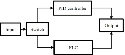
(PID) control and fuzzy logic control (FLC). The method of PID control is simple and the effect of control is good which has been used widely in industrial application. Figure 1 shows the general block diagram of the system to be implemented in this paper. A conventional PID controller is a control loop feedback mechanism. The conventional PID controller has characteristics of simplicity, stable system and high reliability. The PID regulation law can gain a good control effect for quite a number of industrial control objects, especially for linear time-invariant systems control depends on each parameter setting of PID controller. However, PID control cannot set parameter via online. It cannot control well in non-linear and time-varying systems since the parameter is difficult to set [3].However, the methods of fuzzy logic controller (FLC) are getting more and more popular to improve the performance of the system. Therefore, it is necessary to compare the performance between PID control and fuzzy control.

Figure 1: The General Block Diagram Of The System

MATLAB/Simulink is one of the block diagram environment for multidomain simulation. It supports simulation, automatic code generation, and continuous test and verification of the systems [4]. MATLAB/Simulink is used to analyze the performance of the AUV for yaw control. Moreover, Fuzzy logic Toolbox is used for the implementation of the FLC. Fuzzy Logic Toolbox™ provides functions, apps, and a Simulink block for analyzing, designing, and simulating systems based on fuzzy logic [5].

In this paper, the FLC toolbox and Simulink are used to control the AUV for yaw motion. Two methods of control system will be used such as PID control and FLC based on simulation process. The model of AUV come out from system identification technique based on yaw control open loop system [6]. The comparison of simulation results in terms of performances of system response reports in this paper and also can identified the advantages and disadvantages of the two methods. The overshoot,

rise time, settling time in the system response also reported in paper.

2.

A. Proportional-integral-derivative (PID) controller

A PID controller is a control loop feedback mechanism or controller which provides a continuous variation of output to accurately control the process, eliminate the oscillation and improve the efficiency. It is the most common control algorithm used in industry and commonly used as the industrial control system. PID control is also referred to as “Three-term” control which are P for Proportional, I for Integral and D for Derivative as shown in Figure 2. The “Three-term” control responses is calculated and summed up to compute the desired actuator output [6]. PID controller continuously calculates the error value which is the difference between a desired set point and a measured process and applies a correction based on the “Three-term” control.

Figure 2: Block Diagram Of A PID Controller

Proportional Response

4258 further. Hence, the system will become unstable and the oscillation may out of control [7].

Integral Response

Integral (I) represent the past values of the error. For instance, if the current output is not enough strong, the integral of the error will accumulate over a period and the controller will respond by applying a stronger action. The integral component is used to sum up the error term over time. In general, a small error term has its own effect on the integral result. The result is that a small error term will also cause a slightly increase in integral component. The integral response will continually rise over time only if the error is zero, hence the effect is to reduce the steady-state error to nil. During the integral response, the ramp rate which is known as the integral time constant must be longer than the time constant of the process to avoid oscillations [6][7].

Derivative Response

Derivative (D) represent the possible future trends of error based on its current rate of change. The derivative response is proportional to the rate of change of the process value or variable. The derivative component will result a decrease in output if the process variable is increasing rapidly. The control system will react tremendously to the changes in the error term and increase the speed of the overall control system response if there is an increase in derivative time (Tc) parameter. Most of the practical control systems use minute derivative time due to the high degree sensitivity of derivative response towards noise in the process variable signal. If the sensor feedback signal is noisy or the control loop rate is slow, the derivative response will make the control system unstable [6][7].

B. Fuzzy Logic Controller (FLC)

Fuzzy control is a logical system based on fuzzy logic which is much closer in spirit to human thinking and behaviour than traditional logical systems. Fuzzy logic controller (FLC) based on fuzzy logic provides an algorithm which able to convert a linguistic control strategy based on expert knowledge into an automatic control strategy [8-10]. Basically, fuzzy logic captures the approximate, inexact nature of the real world effectively [10-12].

A fuzzy set is represented by a membership function defined on the universe of discourse. It is a generalization of an ordinary set by allowing a degree or grade of membership for each element. A fuzzy set allows the elements in its set to have partial membership in the interval from 0 to 1 [9].

Figure 3: Block Diagram Of Fuzzy Logic Controller

The basic configuration of an FLC comprises four principal components which are fuzzification interface, knowledge base, decision-making logic and defuzzification interface as shown in Figure 3.

Fuzzification

Fuzzification interface is used to measures the values of input variables. Besides, fuzzification interface conducts a scale mapping that transfers the range of values of input variables into corresponding universes of discourse. It also converts the input data into suitable linguistic values which may be viewed as labels of fuzzy sets [8].

Knowledge Base

Knowledge base is made up of knowledge of the application domain and the attendant control goals. A knowledge base contains a data base and a linguistic control rule base. The data base provides required definitions which are used to define linguistic control rule and fuzzy data manipulation in a FLC whereas the linguistic control rule base characterizes the control goals and control policy of the domain experts by a set of linguistic control rules [8].

Decision-making Logic

Decision-making logic is the kernel of a FLC. It is able to simulate the human decision-making based on fuzzy concepts and inferring fuzzy control actions employing fuzzy implication and the rules of inference in fuzzy logic [8].

4259 Defuzzification interface conducts a scale mapping which converts the range of values of output variables into corresponding universes of discourse. It utilizes a non-fuzzy control action from an inferred fuzzy control action [8].

C. Comparison between PID controller and FLC

PID controller has only three parameters (Kp, KI,

and KD) to tune whereas FLC has a lot of

parameters to tune in order to improve the system. The three parameters of conventional PID control need to be constantly adjusted in order to achieve better control performance. The parameters of FLC are adjusted automatically in accordance with the speed error and the rate of speed error-change. FLC has a longer computing time compared to PID controller due to its complex operations such as fuzzification and defuzzification. The main advantage of FLC over conventional PID controller is FLC do not need an accurate mathematical model. Besides, the FLC can work with imprecise inputs and handle non-linearity [9-11].

3. METHODOLOGY

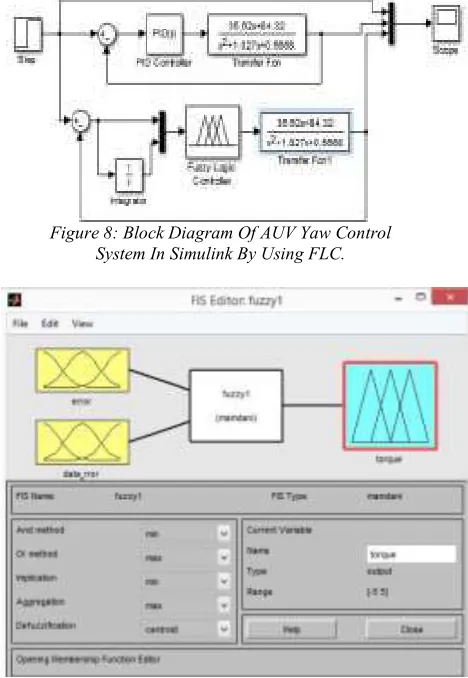
The method used and experimental set-up are discussed thoroughly in this section. At first, the model is given and shown in Equation (1). Next, the model is controlled or tested by using PID controller and Fuzzy Logic Controller through MATLAB software. The purpose of using this both controllers is to make a comparison between their results after tuning and choose the best controller in order to control this model. After that, a block diagram for AUV yaw control system is designed by using Simulink as shown in Figure 4. The circuit is run and simulated without any tuning in order to observe the initial response of the system.

Figure 4: Block Diagram Of AUV Yaw Control System In Simulink By Using PID Controller.

5668 . 0 027 . 1

32 . 84 62 . 35

2_ _



s s

s

TF (1)

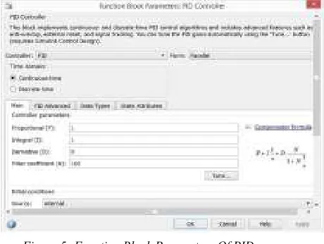
Figure 5 shows the initial parameters of PID controller, where P=1, I=1, D=0, and N=100. Next, the system is tuned by clicking the tune button in

the function block parameters of PID controller and the plant model is obtained by linearizing the plant as shown in Figure 6. After auto-tuning, the final values of PID parameters are generated as shown in Figure 7. The block is updated and the result is shown in the next section. The system result of using PID controller is compared between before tuning and after tuning. Then, the result is compared again with the result of using FLC where both results are discussed in discussion part.

Figure 5: Function Block Parameters Of PID Controller Before Tuning.

Figure 6: PID Tuner.

Figure 7: Function Block Parameters Of PID Controller After Tuning.

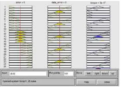
4260 response, a FIS editor is opened by typing ‘fuzzy1’ in the command window of MATLAB. Figure 9 shows there are two inputs and one output in this controller where mamdani inference engine is used for this controller. Input 1 and input 2 are set to error and data error respectively while the output are named as torque. The two inputs and one output are designed with 5 X 5 membership functions and their type of membership functions are set to triangular as shown in Figure 10, Figure 11 and Figure 12 respectively. Each of the partitions for the 5 X 5 membership functions of the inputs and output are designed from Negative Large (NL), Negative Small (NS), Zero (ZE), Positive Small (PS) to Positive Large (PL).

Figure 8: Block Diagram Of AUV Yaw Control System In Simulink By Using FLC.

Figure 9: FIS Editor Of 'Fuzzy1'.

Figure 10: The Membership Function For First Input 'Error'.

Figure 11: The Membership Function For Second Input 'Data Error'.

Figure 12: The Membership Function For Output 'Torque'.

4261

Figure 13: The Rule Editor Of FIS.

Table 1: Rule Table Of FLC For AUV Yaw Control System.

Data Error

PL PS ZE NS NL Error

NL ZE NS NL NL NL

NS PS ZE NS NL NL

ZE PL PS ZE NS NL

PS PL PL PS ZE NS

PL PL PL PL PS ZE The rule statements can be analyzed in another point of view which is called rule viewer as shown in Figure 14. The rule viewer serves as a guidance for the adjustments to be made when tuning the fuzzy logic controller by adjusting the range of the inputs and output. Besides that, Figure 15 shows the surface view of the rules in a three dimensional graph before tuning.

Figure 14: The Rule Viewer Before Tuning FLC.

Figure 15: The Surface Viewer Before Tuning FLC.

6. RESULT AND DISCUSSION

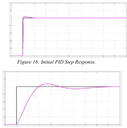
After simulated the circuit of using PID controller, the initial system response is shown in Figure 16 while Figure 17 shows the system response after PID auto-tuning. Based on the graphs shown, black line represents desired response while purple line represents actual response of PID controller. The step response graph for both before tuning and after tuning through PID controller is compared and shown in Figure 18.

Figure 16: Initial PID Step Response.

4262

Figure 18: Initial And Final PID Step Response.

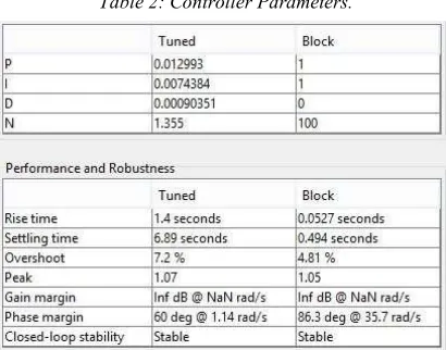
Based on Figure 18, it is clearly shows that the system which used auto-tuning of PID controller has a less smooth response, which is slightly underdamped compared to the initial system response. According to the tuning parameters that shown in Table 2, it can be analyzed that the system which used PID auto-tuning has a higher percentage of overshoot, increasing in rise time, settling time and peak value when compared to the initial setting. Hence, the original PID controller that without using any tuning has a better system response or performance and the result is compared with the system that using FLC in the next part.

Table 2: Controller Parameters.

Next, a FLC is adding to the circuit for the purpose of observing the system response after simulation and make a comparison with the result of using PID controller that without any tuning. The initial response of using FLC is shown in Figure 19 while the system response after manually tuning is shown in Figure 20. As mentioned before, the black line represents the desired response which is as a reference while the purple line represents the system response which is using PID controller. In

addition, the cyan line represents the system response of using FLC.

Figure 19: Comparison Of FLC Response Before Tuning

Figure 20: Comparison Of FLC Response After Tuning And The Initial PID Response.

Based on the Figure 19, the FLC graph shows a very high percentage of overshoot and peak value before tuning where the range is [0 1]. For Figure 20, the system is tuned by FLC and the graph shows that the peak value is scaled down to almost same as the result of initial PID controller system. The tuning process is done which is changing the range values of the inputs and output from [0 1] to [-5 5] in the FIS editor as shown in Figure 21, Figure 22 and Figure 23 respectively. The rule viewer and surface viewer that after tuning FLC are also shown in Figure 24 and Figure 25, respectively. Thus, the system that after FLC tuning is better than its initial response.

4263

Figure 22: The Range Values For Second Input 'Data Error' Is Changed From [0 1] To [-5 5].

Figure 23: The Range Values For Output 'Torque' Is Changed From [0 1] To [-5 5].

Figure 24: The Rule Viewer After Tuning FLC.

Figure 25: The Surface Viewer After Tuning FLC.

Next, the final FLC response which is after tuning is compared with the initial PID response. According to the Figure 20, both PID and FLC shows that the responses are following the set point in the beginning and steady-state. However, there is an overshoot for both responses. The system response of using PID controller shows slightly higher of overshoot than the system response of using FLC. Hence, tuning method is essential to perform in the fuzzy system in order to get a better system performance. Scaling or shifting the membership functions, changing the range values and adjusting the rules are the basic tuning method in FLC system. Therefore, the FLC graph is tuned according to the basic methods mentioned before until a satisfactory response is obtained as shown in Figure 20, where the FLC graph is almost same as the desired response and the percentage of overshoot is reduced when compared with the PID graph. Table 3 shows the comparison of performance of FLC and PID controller.

Table 3: Comparison Of Performance Of FLC And PID Controller.

Parameter FLC PID Tuned PID Block

Rise Time (s) 0.0527 1.4 0.0627 Settling Time (s) 0.494 6.89 0.594

Peak Time (s) 0.15 2.5 0.45 Overshoot (%) 4.81 7.2 4.83 Peak 1.05 1.07 1.06

5. CONCLUSION

4264 that the robustness of Fuzzy Logic Control is better than PID control.

ACKNOWLEDGEMENT

We wish to express our gratitude to honorable University, Universiti Teknikal Malaysia Melaka

(UTeM). Special appreciation and gratitude to

especially for Underwater Technology Research Group (UTeRG), Centre of Research and Innovation Management (CRIM) and Center for Robotics and Industrial Automation for supporting this research and to Faculty of Electrical Engineering from UTeM to give the financial as well as moral support for complete this project successfully.

REFERENCES

[1] Ngatini, E. Apriliani, and H. Nurhadi, “Ensemble and Fuzzy Kalman Filter for position estimation of an Autonomous Underwater vehicle based on Dynamical System of AUV motion, Expert Syst. Application, Vol 68, pp 29-35, 2017.

[2] P. Sarhadi, A. R. Noei, and A. Khosravi, “Adaptive integral feedback controller for pitch and yaw channels of an AUV with actuator saturations,” ISA Trans., vol. 65, pp. 284–295, 2016.

[3] H. Zhang and C. Li, “Simulation and Evaluation of PID Control and Fuzzy Control,” in 2010 International Conference on Electrical and Control Engineering, pp. 1907–1910, 2010.

[4] Simulink - Simulation and Model-Based Design - MathWorks United Kingdom.” [Online]. Available: https://uk.mathworks.com/products/simulink/. [Accessed: 24-Nov-2016].

[5] Fuzzy Logic Toolbox - MATLAB - MathWorks United Kingdom. [Online]. Available:

https://uk.mathworks.com/products/fuzzy-logic/. [Accessed: 24-Nov-2016].

[6] Mohd Aras, Mohd Shahrieel, Hyreil Anuar Kasdirin, Muhamed Herman Jamaluddin, Mohd Farriz Basar, Design and development of an autonomous underwater vehicle (AUV-FKEUTeM), Proceedings of Malaysian Technical Universities Conference on Engineering and Technology, pp 1-5, 2009. [7] Mohd Aras, Mohd Shahrieel, Shahrum Shah

Abdullah, Mohamad Aziz Abd Aziz, Hazriq Izzuan Jaafar, Mohamed Kassim Anuar,

Tuning Process Of Single Input Fuzzy Logic Controller Based On Linear Control Surface Approximation Method For Depth Control Of Underwater Remotely Operated Vehicle, Journal of Engineering and Applied Sciences, Vol. 8, No.6, pp 208-214, 2013.

[8] Mohd Shahrieel bin Mohd Aras, Fara Ashikin binti Ali, Shahrum Shah b Abdullah, Fadilah Abd Azis, Syed Mohammad Shazali Syed Abdul Hamid, Study of the Effect in the Output Membership Function When Tuning a Fuzzy Logic Controller, IEEE International Conference on Control System, Computing and Engineering, 20111.

[6] PID Control and Tuning examples and definitions | Eurotherm, Eurotherm by Schneider Electric | Temperature Control, Process Control, Measurement and Data Recording Solutions. [Online]. Available: http://www.eurotherm.com/principles-of-pid-control-and-tuning. [Accessed: 28-Nov-2016].

[7] Graham C. Goodwin, Stefan F. Graebe, Mario E. Salgado. PID Theory Explained – National Instruments Available:

http://www.ni.com/white-paper/3782/en/#toc2. [Accessed: 28-Nov-2016].

[8] Chuen Chien Lee, “Fuzzy Logic in Control Systems: Fuzzy Logic Controller Part I,” 1990.

[9] Mohammed Shoeb Mohiuddin, “Comparative study of PID and Fuzzy tuned PID controller for speed control of DC motor,” Int. J. Innov. Eng. Technol., Aug. 2013.

[10] Marcelo Godoy of Mines, “Introduction to Fuzzy Control,” Colo. Sch. Mines.

[11] Norhaslinda Hasim, Mohd Shahrieel Mohd Aras, Mohd Zamzuri Ab Rashid, Anuar Mohamed Kassim, Shahrum Shah Abdullah, Development of fuzzy logic water bath temperature controller using MATLAB, IEEE International Conference on Control System, Computing and Engineering (ICCSCE), pp 11-16, 2012.