The Levy sections theorem revisited

Munich Personal RePEc Archive

The Levy sections theorem revisited

Figueiredo, Annibal and Gleria, Iram and Matsushita, Raul

and Da Silva, Sergio

2006

Online at

https://mpra.ub.uni-muenchen.de/1983/

The Levy sections theorem revisited

Annibal Figueiredo1, Iram Gleria2*, Raul Matsushita3 and Sergio Da Silva4

1_{Department of Physics, University of Brasilia, 70910-900 Brasilia DF, Brazil} 2_{Institute of Physics, Federal University of Alagoas, 57072-970 Maceio AL, Brazil} 3_{Department of Statistics, University of Brasilia, 70910-900 Brasilia DF, Brazil}

4_{Department of Economics, Federal University of Santa Catarina, 88049-970 Florianopolis SC, Brazil}

Abstract. This paper revisits the Levy sections theorem. We extend the scope of the theorem to time series and apply it to historical daily returns of selected dollar exchange rates. The elevated kurtosis usually observed in such series is then explained by their volatility patterns. And the duration of exchange rate pegs explains the extra elevated kurtosis in the exchange rates of emerging markets. In the end our extension of the theorem provides an approach that is simpler than the more common explicit modeling of fat tails and dependence. Our main purpose is to build up a technique based on the sections that allows one to artificially remove the fat tails and dependence present in a data set. By analyzing data through the lenses of the Levy sections theorem one can find common patterns in otherwise very different data sets.

PACS: 89.65.Gh; 89.75.−k.

1. Introduction

Recently the study of complex systems has attracted the attention of a growing number of physicists. Scaling laws, self-organized criticality, self-similarity, and fractals, just to name a few, have been found in fields as diverse as biology and economics. These phenomena have created the need for a general theoretical framework to explain them coherently through a physics of complex systems.

A branch known as “econophysics” attempted to explain the self-similarity and fat tails observed in financial distributions that can be responsible for a variety of behaviors and, in particular, ultraslow convergence to the Gaussian regime [1]. Here one major contribution was Mantegna and Stanley’s truncated Levy flight [2], which takes into account both the departures from the classical central limit theorem and the presence of scaling laws.

More recently, we have pursued a different line of research [3, 4]. Rather than looking for underlying probability distributions of financial processes, we focused on the role of nonlinear autocorrelations as well as nonidentically distributed variables. As a result, we could alternatively explain both the ultraslow convergence and scaling laws.

This paper moves forward and suggests an even simpler approach based on the Levy sections theorem [5]. The classical central limit theorem does not take chains of random variables that are dependent into account. Yet the Levy sections theorem is stated under Levy’s generalization of the classical central limit theorem to encompass dependent variables. The Levy sections theorem is not to be confused with his stable distribution of infinite variance. Levy also employed his notion of “sections” to outline a proof for the generalization of the classical central limit theorem in order to consider the sums of dependent random variables [6]. This proof was reworked afterward using less restrictive assumptions [7, 8]. A full description of these developments was presented in his subsequent book [9].

continuous martingale is a time-changed Wiener process, where the time change is the quadratic variation. This is known as the Dambis-Dubins-Schwarz theorem [10, 11, 12]. Also every semimartingale is a time-changed Wiener process [13]. At first, the last result can be employed for discrete time processes (time series). And in particular, asset prices can be considered as time-changed Wiener processes [14, 15]. References on martingale limit theory and the central limit theorem for martingales can be found elsewhere [16, 17, 18].

This paper thus extends the Levy sections theorem’s approach to time series. And we take historical daily returns of selected dollar exchange rates from both developed and emerging markets to illustrate our case. By using the Levy sections to account for local volatilities we find universal patterns in the random behavior of actual financial series. Indeed we explain their stylized fact of elevated kurtosis by the volatilities. And the extra elevated kurtosis of emerging markets is explained by the duration of exchange rate pegs. The longer foreign exchange intervention is, the greater the kurtosis. One can then build a gauge of exchange rate peg duration based on the kurtosis. In the end, our extension of the Levy sections theorem provides an approach that is simpler than the more common explicit modeling of fat tails and dependence [3, 4].

The main purpose of this paper is to build up a technique based on the sections that allows one to artificially remove the fat tails and dependence present in a data set, and then compare this set with a Gaussian one, only to realize that both data sets become very similar if analyzed through the lenses of the Levy sections theorem.

The rest of the paper is organized as follows. Section 2 presents building-block definitions and the Levy sections theorem. Section 3 extends the previous definitions to time series. Section 4 illustrates our framework using data from exchange rate returns. Section 5 puts forward a qualitative gauge of foreign exchange intervention using a Gaussian generator. And Section 6 concludes.

2. Definitions and the Levy sections theorem

We consider a chain of random variables denoted by Xn with n∈ . The conditional probability

of a given realization xn+1 of Xn+1 is written as P x

(

n+1 x1,...,xn

)

. This means the probability of

1

n

x₊ if the random variables X₁,…,X_n follow the particular chain walk x₁,…,x_n. The

conditional mean and variance of X_n+1 are

(

)

1

1 1 1 1,..., 1

n

n Xn _{x x} xn P xn x x dxn n

µ

= + =

∫

+ + + (1)

and

(

)

1 1

2

2 2 2 2

1 1 _n 1 1 1,..., 1

n

n n x x n x x n n n n n

m = X + − X + =

∫

x+P x+ x x dx+ −

µ

. (2)

Both

µ

n and mn depend on x1,...,xn. To simplify notation, we omit the index associated with the

walk dependence. For the chain walk x₁,…,x_n of size n of the random variables X₁,…,X_n we

calculate the quantity

where m_i is the conditional variance of x₁,…,x_i for i=1,…,n. Consider a positive real number

t such that the condition

1

n t n

λ

₋ ≤ <

λ

(3)

is satisfied. We say that the chain walk x1,...,xn belongs to the section t, and condition (3) is

called the section condition t. The

λ

_n−₁ is calculated for the chain walk x1,...,xn−1, i.e.

1 2 1 1 n n i i m

λ

− −

=

=

∑

. For a given chain walk of size n we have

λ λ

i = i−1+m ii2, =2, ,n, and

2 1 m1

λ

= .

The section t is made up of all chain walks obeying the section condition t. Note that the

chain walks can have different sizes n.

The sum x1+ +... xn of elements in a given chain walk belonging to the section t defines a

random variable, denoted by S_t, whose variance is M_t2= S_t2 − S_t 2. The Levy sections

theorem [6−9] is the following.

Theorem. For the null conditional means

µ

n =0 (∀ ∈n ) and random variables Xn (∀ ∈n )

satisfying the Lindeberg conditional condition (see reference [9], section 67, pages 237-246,

theorem 67.3), the probability distribution of S_t/ t is such that

(

)

2

2 1 lim 2 x t

t P S t e dx

η

η

π

−

−∞

→∞ < =

∫

.

Stationarity is not assumed. This theorem extends the classical central limit theorem to consider the

chains of dependent random variables. The distribution of the variable S_t t converges to a

Gaussian of zero mean and unity standard deviation as the section t goes to infinity. The

normalized variable S Mt t, with

2 2

t t t

M = S − S , also converges to the Gaussian of zero

mean and unity standard deviation. For a given section t, the variable S_t t (unlike S M_{t t}) has

not unity standard deviation. Yet both variables have the same skewness and kurtosis (and the same is true of the other reduced statistical moments). Both converge to a normal distribution of unity

standard deviation. While the standard deviation of S M_{t t} remains constant and equal to unity

over the convergence process, the standard deviation of S_t t changes, yet converging

asymptotically to unity.

Given the conditional probability of the random variable X_n, its probability distribution is

given by the marginal probability defined as

(

)

1 1

1 1

( ) ,...,

n

n n n n

x x

p x P x x x

−

−

=

∑

where the sum considers all possible walks x1,...,xn−1 followed by the random variables

1,..., n1

(

)

2 2

2 2 2

( ) ( )

n Xn Xn x p x dxn n n n x p x dxn n n n

ν

= − =

∫

−

∫

.

Let us define the quantity

2 2 1 n n i i n

σ

ν

= ≡

∑

which we call the cumulated average variance of Xn. Then, let us consider the sum random

variable Sn of size n defined in the usual way, i.e.

1

n n

S =X + +X . (4)

Its variance, M_n2 = S_n2 − S_n 2, satisfies

2 2

1 1

cor( , )

n n

n i i j i j

i i j

M

ν

X X

ν ν

= ≠ =

=

∑

+

∑

,

where cor(X X_i, _j) is the linear correlation between variables X_i and X_j.

Next we define the quantity

2 2

n Mn n

τ

=

σ

which we call the variance time of S_n. To understand its meaning first consider the example of a

chain of independent random variables X_n, where cor(X X_i, _j)=0 for all i≠ =j 1,…,n, and

n n

τ

= . The variance time is just the “actual” time n.

Another example shedding light on the meaning of the variance time of S_n is a situation

where the marginal variance

ν

_i2 is stationary, i.e.

ν

_i2 =

ν

2 for all i∈ . In this case the variance

time becomes

2

2

1

cor( , ) n

n

n i j

i j M

n X X

τ

ν

≠ =

= = +

∑

.

Note that the presence of linear correlations can lead to delays and advances in the variance time

when compared to the actual time n. For some chains (for example, Mandelbrot’s fractional

Brownian motion) the variance of S_n may follow a scaling law such as M_n = AnH, where H is

Hurst exponent. Here the variance time is

τ

_n =n2H. If H >1/ 2 (H <1/ 2) the variance time

will move ahead (fall behind) the actual time.

We do not attach an index related to the actual time in the random variable St because the

number of terms in S_t depends on the chain walk. Yet the size n of a chain walk x₁,…,x_n

We denote it by n_t. If the variance of X_n is stationary, the variance time (associated with the

section)

τ

t of St is

2 2

t Mt v

τ

= .

3. Extending the concepts to time series

A time series

( )

x_{i i=1,...,N}, where i is a time counter and N is the series size, can be thought of as a

single realization of a random process. We can employ to this series either (1) the technique based

on the marginal probability of a chain of identical random variables [3−6] applied to study of the

properties of Sn or (2) the properties associated with the sum St as defined in Eq. (4). The

technique uses the concept of conditional variance mn of a given chain of random variables as well

as the variable S_t introduced in Section 2. To clarify the differences between the two approaches

we elaborate further on the definitions associated with S_n and S_t.

For the time series we rewrite the sum Sn for a given n<N as

1

1 1 1

, , ,

n n n

n i i N n i

i i i

S x x₊ x _{− +}

= = =

 

=  



∑ ∑

∑

.

Such collection of sums is seen as one realization of S_n =X₁+ +X_n, where the random

variables Xi with i=1,…,n are identically distributed. The original time series is only one of the

all possible realizations, i.e. X_i= X =( ,x x_{1 2},…,x_N). The marginal variance

ν

2 = X2 − X 2

can be straightforwardly reckoned from the list X. This allows one to calculate the variance time

2 2

n Mn

τ

=

ν

, where M_n2 is the variance of S_n. Thanks to the presence of correlations, the

normalized Sn does not converge to a Gaussian.

One big difficulty is learning the values taken by the local volatilities m_i2 since it is

impossible to get them from only one realization of the variable, namely the empirical value of xi

taken from the data set. For this reason we need an extra technique to calculate the local volatilities.

So consider a positive integer q, and the new time series

( )

yn n=1,...,N−2q,

where the first and the last q terms of

( )

x_{n n=1,...,N} were dropped, i.e. y_n =x_{n q+} , 1,...,n= N−2q.

Then the local volatility mn2 is

2 2 2 2 2 1 2 1 1 2 1

∑

+

∑

= + =      + − +

= n q

n i q n n i i i n x q x q

for n=1,…,N−2q. Here the local volatility is a measure of the conditional variance associated with a given chain of random variables.

Thus we can extend the concept of the Levy section t for the collection

( )

y_{n n=1,...,N−2q}. The

t

S ends up as the collection of all the sums

{

}

1 ... _i 1 _i, 1,..., 2

i i n n

y +y₊ + + y ₋ +y i∈ N− q

such that the condition in Eq. (3) is fullfilled, i.e.

2 2 2 2 2 2

1 1 ... 1 1 ...

i i i i

n mi mi mn t mi mi mn n

λ

− = + + + + − ≤ < + + + + =

λ

,

where every mi2 is calculated by Eq. (5).

The local volatility definition implies the existence of an integer j_t∈

[

0,N−2q

]

such that

the section condition t is not fulfilled for i> j_t. Indeed, j_t is the number of elements belonging to

the collection S_t which can be rewritten as

1 2

1 1

1 1 1

, , ,

jt

t n

n n

t i i j i

i i i

S y y₊ y _{− +}

= = =

 

= _ _



∑ ∑

…

∑

.

For every section t we can define the collection nt =( ,n n1 2,…,nj_t) made up of the number of

terms in every sum belonging to the collection St.

For the time series, the variance of S_t is M_t2 = S_t2 − S_t 2, and the variance time of S_t

is

τ

t =Mt2 v2. Also, the average number of terms associated with St is nt =(n1+ +nj_t) jt .

The purpose of the definition of variance time is to compare the time evolution of both S_n and S_t.

Unlike Sn, the St is not indexed to actual time, i.e. no particular time is associated with it. The

scale of the variance time, however, allows one to compare the two. Although other scales can be

imagined, in the one suggested here the variance of both S_n and S_t is the same for every variance

time. So we can assess the evolution of Sn and St by considering not actual time, but how their

respective variances evolve.

We assume that the time series is stationary when doing the sum procedures above. Though the stationarity assumption for a chain of random variables is not made in the Levy sections

theorem, our sum procedures to obtain S_t for an empirical time series make sense only if the series

is stationary. So our sum procedure is to be blamed in the event of a possible failure of the extension of the Levy sections theorem to time series.

4. Illustrating with exchange rate returns

returns, i.e. x_n = −r_n r_n−1, where rn is an exchange rate (dollar price of a foreign currency) at date n.

The data are collected from the Federal Reserve website. Table 1 gives more details.

We reckon the local volatility of trading weeks (5-day weeks), which means q=2 in

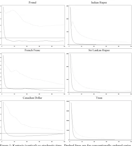
Section 3’s formulas. Figure 1 shows the kurtosis K as a function of the variancetime. Dashed

lines are the kurtosis’ evolution of the conventionally ordered series S_n as a function of

τ

_n. The

continuous lines are the kurtosis’ evolution of S_t as a function of

τ

_t.

To display the kurtosis behavior of the sections sums, we start with the initial (very small)

section t=10−15, and then calculate the sections t+ ∆i t, for i=1,…, 99. We cannot pick the

section t=0 to begin with because of computational limitations. The values of ∆t are arbitrarily

chosen to enable one to see smooth variations of the kurtosis as well as the transient period of kurtosis evolution. We restrict the calculations to 100 steps because this is enough to assuring the asymptotical convergence of the kurtosis. And also because this allows one to keep the number of

terms of the sums in St small if compared to the original number of terms in an empirical time

series. This prevents introducing spurious correlations among the terms in sequence S_t. The values

of ∆t used in every currency are in Table 2. The key features shown in Figure 1 are as follows.

(A) There is kurtosis convergence in the sections sums S_t of the currencies toward a well

defined asymptotic state. This does not hold in the sums S_n of the conventionally ordered

exchange rate time series.

(B) The variance time of kurtosis convergence for the sections sums is short. Unlike in the

conventionally ordered sums, the kurtosis convergence for the sections is similar for all

rates. All the sections kurtosis practically reached the limit at the variance time

τ

_t =10.

(C) The kurtosis convergence approaches zero. Developed countries’ currencies present

slightly negative kurtosis and emerging countries’ currencies have slightly positive kurtosis. Unlike in the conventionally ordered series, the sections sums converge to a distribution resembling the Gaussian.

(D) The sections’ kurtosis evolution presents a universal behavior for the currencies studied,

regardless of the fact that a country is developed or not.

What happens from the perspective of actual time? Assuming the variance time

τ

=10 as

an equilibrium benchmark, we can take the section t corresponding to that time for every currency.

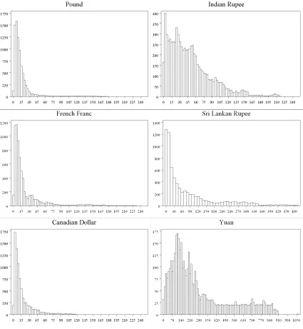
Table 3 lists the values of t for the exchange rate series. We can obtain the collection n_t as

defined in Section 3, and also calculate n_t : the average number of terms of the sums of section t.

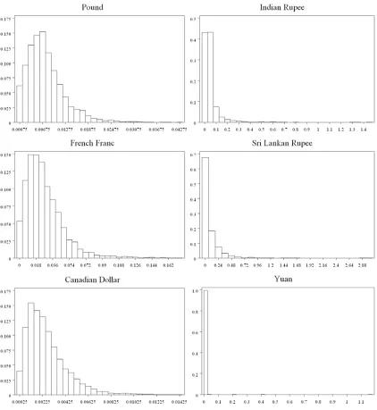
Figure 2 shows histograms of the collections n_t, and Table 4 presents n_t for the exchange rates.

Compared to the histograms of emerging markets’ currencies, the histograms of developed

markets’ currencies tend to cluster in a near-zero value. And the average number of days nt

corresponding to the stationary limit

σ

_t =10 of the sections t of developed countries’ currencies is

smaller than that of emerging markets’ currencies (the values of t are those displayed in Table 3).

These features may be related to the degree of government intervention in the emerging markets’ currencies. A fixed exchange rate regime would mean zero volatility (constant rate) and a return series dominated by zeros. China, for instance, kept an 11-year-old peg of its currency, the yuan, at 8.28 to the dollar. But there were also four big episodes of revaluation in the yuan-dollar returns’ series considered. This caused an interesting effect. Because volatility nears zero most days, one

t

n greater than that of the other currencies. Indian and Sri Lankan rupees present smaller values

but still greater than those of the pound, French franc, and Canadian dollar. The developed

countries’ currencies exhibit very similar n_t .

Figure 3 shows histograms related to the currencies’ local volatility. The yuan’s volatility clusters in zero, unlike those of developed countries’ currencies. This explains the observed

patterns in the histogram of n_t (Figure 2).

5. A suggested gauge of exchange rate control

As an exercise, we put forward a qualitative gauge of foreign exchange intervention using a Gaussian generator. Consider a Gaussian random generator of reduced variables that are

independent and identically distributed (IIDR) [4]. Then consider the sequence zn =m gn n,

1,..., 2

n= N− q (with q = 2 in the empirical example), where gn is generated by a normal

distribution, and m_n is the local volatility. What is special here is that the volatility process is not

modeled, but taken from the data. If m_n is constant, the distribution of z_n =m g_{n n} collapses to a

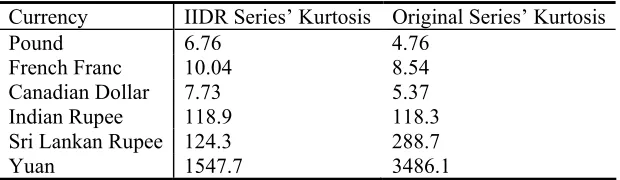
Gaussian. The column in the middle of Table 5 shows the kurtosis of the IIDR applied to the exchange rates. The right hand side column shows the kurtosis of the original series of daily returns. The effect of the local volatilities is unambiguous. Because the generator is Gaussian, the elevated kurtosis should be explained by the volatilities.

Thanks to exchange rate pegs, return dispersion is low at the days a rate is fixed. Thus a number of return observations fall out of the variance interval (by variance interval we mean the symmetric interval around the mean that is two standard deviation wide, and with respect to the original returns series; and this without taking the sections into account). The elevated kurtosis in emerging markets’ exchange rates can then be explained by too many observations outside the variance interval. This rationale is simpler than the more usual ones based on fat tails and dependence. The Levy sections filter the effects on the local volatility so that the return series present a near-Gaussian universal pattern.

Exchange rate time series are commonly believed to be modeled by a Gaussian whenever

government intervention is absent. This is because government intervention introduces patterns in

the series that can be exploited by market participants to improve their forecasts. With free float the market is more likely to be efficient in the sense that the properly anticipated prices fluctuate randomly [19]. Our results show that foreign exchange intervention provokes departures from the Gaussian in that it biases the volatility evolution. So the greater the control is, the greater the kurtosis. This is so because the pegs tend to bring a series’ dispersion closer to zero, thereby rendering many observations out of the distribution’s variance interval. Thus the kurtosis reckoned in the IIDR can be seen as a gauge of peg duration. Normalizing the pound-dollar’s kurtosis to unity, we can get a relative intervention scale (Table 6). Note that this gauge is qualitative in that no quantitative relation between the kurtosis ratios and the peg durations are provided. This might be one interesting topic for future research.

6. Conclusion

returns of selected dollar exchange rates, we calculate the local volatilities of their trading weeks. Doing so, we find a universal behavior in the actual series.

Unlike in the conventionally ordered exchange rate time series, we find kurtosis convergence toward a well defined asymptotic state in their correspondent Levy sections. We also find the time of kurtosis convergence to be short. This is similar for the currencies considered. The kurtosis convergence approaches zero. And in the Levy sections, the convergence occurs toward a distribution resembling the Gaussian.

As an exercise, we employ our approach to show that the extra elevated kurtosis of emerging markets’ exchange rates can be explained by too many observations outside the variance interval. This is so thanks to the duration of exchange rate pegs. Foreign exchange intervention provokes departures from the Gaussian in that it biases the volatility evolution. So the greater the control is, the greater the kurtosis.

We finally suggest a qualitative gauge of peg duration based on the kurtosis reckoned in the Gaussian generator, and leave the search for a quantitative gauge for future research.

Acknowledgements

Annibal Figueiredo, Iram Gleria, and Sergio Da Silva acknowledge financial support from the

Brazilian agencies CNPq and CAPES−Procad.

References

[1] Mantegna R N, Stanley E 1995 Scaling behaviour in the dynamics of an economic index Nature

376 46 – 49.

[2] Mantegna R N, Stanley E 1994 Stochastic processes with ultra-slow convergence to a Gaussian:

the Truncated Levy Flights Physical Review Letters73 2946–2949.

[3] Figueiredo A, Gleria I, Matsushita R, Da Silva S 2004 Levy Flights, autocorrelation and slow

convergence, Physica A337 369−383.

[4] Figueiredo A, Gleria I, Matsushita R, Da Silva S 2006 Nonidentically distributed variables and

nonlinear autocorrelation Physica A363 171−180.

[5] Levy P 1935 Proprietes asymptotiques des sommes de variables aléatoires enchainees, Bull. Soc.

Math. 59 1−32.

[6] Levy P 1934 L’addition de variables aléatoires enchainees et la loi de Gauss Bull. Soc. Math.

FranceC. R. des Seances62 42−43.

[7] Levy P 1934 Proprietes asymptotiques des sommes de variables aleatoires enchainees C. R.

Acad. Sci.199 627−629.

[8] Levy P 1935 La loi forte des grands nombres pour des variables enchainees C. R. Acad. Sci.201

[9] Levy P 1937 Théorie de l’addition de variables aléatoires, Gauthiers-Villars, Paris.

[10] Dubins L E, Schwarz G 1965 On continuous martingales Proc. Nat. Acad. Sci. U.S.A.53, 913–

916.

[11] Dambis K E 1965 On the decomposition of continuous submartingales Theor. Probab. Appl.

10, 401–410.

[12] Klebaner F C 1998 Introduction to stochastic calculus with applications, Imperial College Press, London.

[13] Monroe I 1978 Processes that can be embedded in Brownian motion Ann. Probab.6, 42−56.

[14] Clark P 1973 A subordinated stochastic process model with fixed variance for speculative

prices Econometrica41, 135–156.

[15] Geman H, Madan D, Yor M 2001 Asset prices are Brownian motion: only in business time, in Quantitative analysis in financial markets, Avellaneda M (ed), World Scientific, River Edge, NJ, 103–146.

[16] Tong H 1990 Non-linear time series, Oxford Science Publishers, New York.

[17] Hall P, Heyde C C 1980 Martingale limit theory and its applications, Academic Press, New York.

[18] Pollard D 1984 Convergence of stochastic processes, Springer-Verlag, New York.

[19] Samuelson P A 1965 Proof that properly anticipated prices fluctuate randomly, Industrial

[image:12.595.153.453.142.233.2]

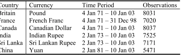
Table 1. Description of data.

Country Currency Time Period Observations

Britain Pound 4 Jan 71 – 10 Jan 03 8031

France French Franc 4 Jan 71 – 31 Dec 98 7020

Canada Canadian Dollar 4 Jan 71 – 10 Jan 03 8037

India Indian Rupee 2 Jan 73 – 10 Jan 03 7525

Sri Lanka Sri Lankan Rupee 2 Jan 73 – 10 Jan 03 7171

China Yuan 2 Jan 81 – 10 Jan 03 5471

Table 2. Values for steps ∆t.

Currency ∆t

Pound 0.00002

French Franc 0.00031

Canadian Dollar 0.0000023

Indian Rupee 0.054

Sri Lankan Rupee 0.02

Yuan 0.00055

Table 3. Value of

t

for the section corresponding to τt =10.

Currency t

Pound 0.00046

French Franc 0.00682

Canadian Dollar 0.0000506

Indian Rupee 0.0584

Sri Lankan Rupee 0.1

Yuan 0.01210

Table 4. Values of n_t for τt =10.

Currency n_t

Pound 15.04

French Franc 23.13

Canadian Dollar 17.26

Indian Rupee 246.20

Sri Lankan Rupee 79.06

[image:13.595.144.454.141.231.2]

Table 5. Kurtosis of the Gaussian IIDR and of the original series.

Currency IIDR Series’ Kurtosis Original Series’ Kurtosis

Pound 6.76 4.76

French Franc 10.04 8.54

Canadian Dollar 7.73 5.37

Indian Rupee 118.9 118.3

Sri Lankan Rupee 124.3 288.7

Yuan 1547.7 3486.1

Table 6. Intervention scale: IIDR series’ kurtosis relative to IIDR pound-dollar return series’ kurtosis.

Currency Intervention Scale

Pound 1.0

French Franc 1.48

Canadian Dollar 1.14

Indian Rupee 17.60

Sri Lankan Rupee 18.39

[image:14.595.84.507.102.570.2]

[image:15.595.84.509.104.565.2]

[image:16.595.84.506.102.561.2]