A Fast Iteration Method for Mixture Regression Problem

http://dx.doi.org/10.4236/jamp.2015.39136

A Fast Iteration Method for Mixture

Regression Problem

Dawei Lang, Wanzhou Ye

College of Sciences, Shanghai University, Shanghai, China Email: [email protected]

Received 7 July 2015; accepted 5 September 2015; published 8 September 2015

Copyright © 2015 by authors and Scientific Research Publishing Inc.

This work is licensed under the Creative Commons Attribution International License (CC BY). http://creativecommons.org/licenses/by/4.0/

Abstract

In this paper, we propose a Fast Iteration Method for solving mixture regression problem, which can be treated as a model-based clustering. Compared to the EM algorithm, the proposed method is faster, more flexible and can solve mixture regression problem with different error

distribu-tions (i.e. Laplace and t distribution). Extensive numeric experiments show that our proposed

method has better performance on randomly simulations and real data.

Keywords

Mixture Regression Problem, Fast Iteration Method, Model-Based Clustering

1. Introduction

In some situations, the data may not be suitable for the linear model, such as nonlinear regression, nonparame-tric regression, generalized linear model. The mixture regression problem discussed in this paper is a situation with mixed data. Specifically, in the observations, some data are from a model, while others are from other models. As in [1], mixture regression problem can be treated as a regression or a clustering problem which can be written as:

, 1, 2, ,

k k

Y =X′β +σ ε k= g

(

)

ik P xi k

π = ∈ Ω (1.1)

where X∈Rp n× is an independent variable matrix, Xj∈Rn, j=1,,p are the observations of the jth va- riable. p, 1, ,

i

x ∈R i= n is the ith observation of the data. Y =

(

y₁, , y_n

)

′∈Rn is response variable vector.

p

k R

β ∈ and σ ∈k R k, =1, 2, ,g are unknown vectors of regression coefficients and unknown positive

of observation x_i belong to population Ω_k (i.e. π_ik =P

(

x_i∈Ω_k

)

. So

1 1

g ik

k=π =

∑

.

The Equation (1.1), a mixture regression model, can also be treated as a model-based clustering [2], which can be solved by an EM Algorithm [3]-[5]. In fact, EM Algorithm is a statistical method for maximizing the li-kelihood function by iterative method. The algorithm can be divided into two steps. The one is E-step which is used for estimating the exception for the parameters. The other one is M-step, which is used for maximize the likelihood function under the parameters predicted in E-step. The iteration will continue until the change of like-lihood function is less than a given value (i.e. 10−6).

In [6], Song used an EM algorithm for solving robust mixture regression model. The details of this algorithm are described as follows:

• Initialize the value of the parameters:

(

2 2

)

1, 1, 1, , g, g, g

θ = β σ π β σ π (1.2)

• E-Step: At the (k + 1)th iteration, calculate:

( ) ( )

(

( ) ( )

)

( ) ( )

(

( ) ( )

)

1 1 1 exp 2 exp 2

k k k k

i i j j i i

ij _{g k k k k}

m m j j m m

m

Y X

Y X

π σ β σ

τ

π σ β σ

− − = ′ − − = ′ − −

∑

∣

∣ (1.3)

( ) ( ) 2 k i ij _k

j j i

Y X σ δ β = ′

− (1.4)

• M-Step: Use the following value:

( ) ( 1) ( 1)

_{( )}

( 1) 1 ( 1)

_{( )}

( 1)

1

1 1 1

1 ,

n n n

k k

k k k k

k

i ij i ij j j ij j j

j j j

ij X X ij X Y

n

π τ β τ δ τ δ

− + + + + + + = = =    ′ ′     = = _{ }  

∑

∑

∑

(1.5)

( ) ( )

_{( )}

( )

(

( )

)

( ) 2 1 1 1 1 2 1 1 2 1

n k k k

ij j j i

j k

i n k

j ij

ij Y X

τ δ β

σ σ τ + + + = + + ′ − = =

∑

(1.6) to maximize:

(

)

2

2

2

1 1 1 1 1 1

1

log log

2

g g g

n n n

ij ij j j i

ij i ij i

j i j i j i i

Y X

τ δ β

τ π τ σ

σ

= = = = = =

′ −

− −

∑∑

∑∑

∑∑

(1.7)

Solving mixture regression problem based on EM algorithm is a complex work with large amount calculation in each iteration. In this paper, we propose a Fast Iteration Method inspired by k-means clustering [7] to solve the mix regression problem. The aim of our method is to fit the data into several linear models. It can also be treated as a model that uses several lines to explain the data (See Figure 1). We will introduce this Fast Iteration Method in the next section.

2. Fast Iteration Method

2.1. Existence of Parameter Matrix

For the situation of the mixture regression problem, the aim of this problem is to find several linear models (i.e. every parameter βk of the model). While, if we known whether an observation is belong to each population, mixture regression model can be treated as a simple linear model. That is: there exist β₁,,βa to minimize the square error. We give a theorem as follows.

Theorem 2.1 The existence of the parameter matrix

β

. In the mixture regression problem, there exists a parameter matrix

β

which can minimize the square error.

Proof τ_ik∈

{ }

1, 0 is given which stand for the ith data which belong to Ω_k or not. If τ is fixed, the model can be written as:

1 0 1

p g

n

i ij jk ik

i j k

y x β τ

= = =

[image:3.595.120.512.87.381.2]

Figure 1. Three lines example for mixture regression problem.

If we know every τ_ij, this model is a linear model. For example, if there are two models Ω₁ and Ω₂ in which includes one variable (p = 1, g = 2). The full model can be described as:

1 2

1 0 1 n

i ij jk ik

i j k

y x β τ

= = =

=

_∑∑∑

1 11 1 01 1 1 12 2 02 2

i i i i i i i

y =x β τ +β τ +x β τ +β τ (2.2)

If the elements τ_ik of matrix τ are given, the problem is the same as a linear regression model. As τ_ik is 0 or 1, so that matrix τ has limited combinations: 2ik.

For the limited combinations, there exists a combination which will lead to the minimum square error.

2.2. Fast Iteration Method for Mixture Regression Problem

EM algorithm is meaningful to the mixture regression problem. However, there are still some other methods to solve this question.

The algorithm below is a fast iteration for mixture regression model, which could solve the regression situa-tion with data in different populasitua-tions. This method is inspired by K-means (the famous clustering algorithm) which calculate the distance between each point to other models and replace the “worst” observation to the suit-able model. After finishing this type of calculation for several times, the algorithm will stop until moving any points to other model won’t make the loss-function better, that is, the change of loss function will below a thre-shold (10−6 or 10−9). In the question of small samples, this stop rules will lead to find a best classifying: moving any observation to any other populations will make things worse. Sometimes set a threshold will avoid the algo-rithm fall into the endless loop.

Our proposed Fast Iteration Method is similar to K-means algorithm, calculate the MSE for each point to every model and change the point which can decrease the MSE most. We summarize our method as follows.

Algorithm:

parts

(

Ω ,Ω , ,Ω_{1 2} _g

)

, every part has about

[ ]

n g observations.

2) Get the subset: X1=

{

x i_i, ∈Ω , 1₁

}

Y =

{

y i_i, ∈Ω , ,₂

}

 Xg=

{

x i_i, ∈Ω ,_g

}

Yg=

{

y i_i, ∈Ω ._g

}

3) Fit g linear models from Ω ,Ω_{1 2} to Ω_g

1 1 2 2 , Ω , Ω , Ω i i i i

i i g g

y x i

y x i

y x i

β ε β ε β ε = + ∈ = + ∈ = + ∈ 

And get β β₁, ₂, ,β_g. 4.) Calculate:

(

,

)

i F X Y

β =

(

) (

2

)

2

.

ik i i wi i i k

judge = y −xβ − y −xβ

5)

{ }

{

}

,

, argmax ik

i k

I K = judge Move observation I to population K, so that we can refresh the Ω ,Ω_{1 2},,Ω_g:

. I W =J

6) Repeat 2 - 5 until stop

For the method of parameter estimating in the algorithm, F X Y

(

,

)

can be changed according to the differ-ent situations. For example, if we want to get the OLS estimation the F X Y

(

,

)

can be:

(

)

( )

1 ,

linear i i i i

F X Y X X X Y

−

′ ′

=

If we need a robust estimation, F X Y

(

,

)

can be a method like median regression. Different methods for pa-rameter estimation make the model much more flexible. OLS estimation can be solved quickly and median re-gression performs better if ε draw from a Laplace or t distribution.

3. Simulation

3.1. Numeric Simulation

In order to validate the rationality of the model, we designed a numeric simulation and generated sample data

(

x yi, i

)

ni=₁ in these three models.

Model 1

1

1

1 , if 1 1 , if 2

X g Y X g ε ε + + =  = _{− + + =}  Model 2 1 1

1 , if 1 1 , if 2

X g Y X g + + =  =  _{− + =}  ε ε Model 3

1 2 1

1 2 1

0 , if 1

0 , if 2

X X g

Y

X X g

+ + + =  =  _{− − + =}  ε ε

For every model considered above, we generated sample using different kinds of distributions: 1) ε~N(0,1); 2)

ε~a Laplace distribution with mean 0 and variance 1; 3)ε~0.95N(0,1) + 0.05N(0,25) Mixture Normal distribution; 4) ε~t3 t-distribution with degree 3.

We used three methods for comparing. Fast Iteration with Linear Model (FI-OLS), Fast Iteration with median regression model (FI-LAE) and EM algorithm are used for solving mixture regression problem for each model.

[image:5.595.87.537.96.403.2]

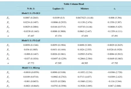
Table 1. Bias (MSE) of point estimates for model 1, n = 100.

Table Column Head

N (0; 1) Laplace (1) Mixture t3

Model 1 1: FI-OLS

10

β 0.0087 (0.2045) −0.0109 (0.5) 0.0637623 (14.40) −0.008 (5.394)

11

β 0.0234 (0.1407) −0.0086 (0.2935) −0.1150 (2.476) 0.1550 (5.387)

20

β 0.0029 (0.2004) 0.0146 (0.5715) −0.0710 (14.46) −0.0606 (5.425)

21

β −0.0338 (0.1463) 0.0088 (0.3008) 0.0863 (2.447) −0.1359 (4.111)

n 47.447 47.374 47.654 47.491

Model 1 1: FI-LAE

10

β 0.0058 (0.1346) 0.0059 (0.1904) 0.0690 (9.369) −0.0029 (0.2625)

11

β 0.036 (0.1005) 0.0431 (0.1444) 0.1024 (2.555) 0.0326 (0.1920)

20

β −0.008 (0.1467) 0.0026 (0.1861) −0.0503 (9.676) −0.0084 (0.2812)

21

β −0.037 (0.1034) −0.0497 (0.1259) −0.2064 (2.584) −0.0449 (0.1863)

n 47.772 47.505 48.505 47.795

Model 1 1: Mixreg

10

β −0.0018 (0.0559) 0.0090 (0.5108) −0.1052 (12.54) −0.0306 (2.720)

11

β 0.0109 (0.0710) −0.0982 (0.2763) 0.5713 (4.657) −0.0309 (2.425)

20

β _{−0.001 (0.0653)} 0.0155 (0.5280) −0.1060 (12.01) −0.116 (3.544)

21

β −0.0021 (0.0645) −0.0792 (0.3598) −0.3928 (3.095) 0.067 (2.068)

model 1, Table 2 for model 2 and Table 3 for model 3)

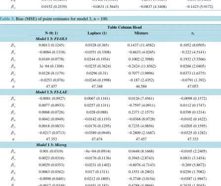
As we can see in the three tables, simulation shows the Fast Iteration for Matrix Regression with LAE per-forms better in Laplace distribution and t-distribution. More specifically, in Table 1, FI-LAE has the smaller MSE in Laplace distribution, Mixture normal distribution and t distribution. EM algorithm gets a better estima-tion in normal distribuestima-tion. In Table 2, FI-OLS performs better in normal distribution which got a smaller MSE than FI-LAE and EM algorithm. In other distribution in model 2, FI-LAE is better than FI-OLS and EM algo-rithm got the biggest MSE. In Table 3, we can also see the FI-LAE got a small MSE in mixture and t distribu-tion, while in the situation of Laplace distribudistribu-tion, FI-LAE is a little bit better than EM algorithm.

As we described our model as a “fast” iteration method, the FI-OLS and FI-LAE are calculated faster than EM algorithm. For 100 observations with 2 populations, EM got about 0.07 s for mixture regression (Rpackage: Mixreg), while FI-OLS used about 0.02 s (i5, 8G memory).

3.2. Real Data Simulation

In the data simulation section, we use the data by Cohen (1984) [8]. A data shows pure fundamental tone was played to a trained musician. 150 observations of tuned and stretch ratio are played by the same musician. In this section, we will see the FI-LAE algorithm will handle the mixture regression data with outliers.

• Situation 1: Original data.

• Situation 2: Data with 5 outliers at (3,5).

• Situation 3: Data with 5 outliers at (1.5,0).

• Situation 4: Data with 5 outliers at (0,5) (Figure 2).

[image:6.595.86.538.101.359.2]

Table 2. Bias (MSE) of point estimates for model 2, n = 100.

Table Column Head

N (0; 1) Laplace (1) Mixture t3

Model 1 2: FI-OLS

10

β 0.067 (0.127) 0.2335 (0.2649) 2.596 (8.789) 0.4682 (3.3621)

11

β 0.0074 (0.1797) 3e−04 (0.288) −0.0584 (3.2318) 0.0242 (4.3117)

20

β −0.0608 (0.1325) −0.2487 (0.2763) −2.5688 (8.5827) −0.4789 (4.7674)

21

β 0.0243 (0.1991) −0.031 (0.3553) 0.0199 (2.698) 0.0501 (6.8493)

n 48.294 48.533 48.304 48.32

Model 1 2: FI-LAE

10

β −0.0813 (0.1561) −0.0017 (0.1509) 1.8594 (5.5725) 0.0027 (0.2078)

11

β −0.0162 (0.2411) −0.0025 (0.273) −0.002 (3.2212) 7e−04 (0.3315)

20

β 0.0942 (0.1627) −0.0047 (0.1545) −1.8665 (5.5066) 0.0011 (0.1907)

21

β 0.0284 (0.2515) −0.0087 (0.2756) 0.0376 (3.4155) 0.0122 (0.3787)

n 47.772 47.505 48.505 47.795

Model 1 2: Mixreg

10

β −0.1892 (0.4177) −0.2054 (1.3923) 1.3117 (8.5285) 0.0722 (5.718)

11

β 8e−04 (0.3108) −0.0452 (1.4686) 0.01 (4.8435) 0.0018 (10.1499)

20

β 0.1731 (0.4249) 0.1488 (1.3561) −1.2019 (7.9067) 0.093 (3.1488)

21

[image:6.595.88.536.334.711.2]

β 0.0152 (0.2539) −0.0631 (1.5643) −0.0837 (4.3408) −0.1423 (5.9172)

Table 3. Bias (MSE) of point estimates for model 3, n = 100.

Table Column Head

N (0; 1) Laplace (1) Mixture t3

Model 1 3: FI-OLS

10

β 0.0013 (0.1245) 0.0328 (0.365) 0.1437 (11.4582) 0.1052 (8.0505)

11

β −0.0084 (0.1318) −0.0351 (0.3308) −0.6633 (4.0265) −0.222 (4.5141)

12

β 0.0169 (0.0778) 0.0244 (0.1954) 0.1002 (2.3988) 0.1932 (3.5566)

20

β 3e−04 (0.1308) −0.0235 (0.3624) −0.2424 (11.8562) 0.0266 (2.0405)

21

β 0.0128 (0.1179) 0.0296 (0.31) 0.7077 (3.9896) 0.0373 (1.6375)

22

β −0.0253 (0.076) −0.0246 (0.1998) −0.187 (2.4352) −0.0791 (1.392)

n 47.457 47.348 46.584 47.053

Model 1 3: FI-LAE

10

β −0.0081 (0.0927) 0.0067 (0.1161) 0.0126 (7.4561) −0.0098 (0.1572)

11

β 0.0077 (0.0933) 0.0257 (0.1311) −0.7597 (4.0911) 0.0112 (0.1747)

12

β 0.0068 (0.0726) 0.028 (0.088) 0.2371 (2.1575) 0.0398 (0.1214)

20

β 0.0042 (0.0949) −0.0142 (0.1193) −0.0368 (8.0728) −0.0102 (0.1622)

21

β 0.0018 (0.0833) −0.0176 (0.1295) 0.7235 (4.0856) −0.0205 (0.1595)

22

β −0.0217 (0.0713) −0.0389 (0.0949) −0.2809 (2.1687) −0.0325 (0.1282)

n 47.353 47.674 47.457 47.333

Model 1 3: Mixreg

10

β 0.001 (0.0319) −8e−04 (0.0914) 0.0448 (8.1668) −0.0165 (2.2405)

11

β 0.0023 (0.0316) −0.0176 (0.1136) 0.3945 (2.8743) 0.0831 (3.1454)

12

β 0.0029 (0.0353) −0.0231 (0.1402) −0.6076 (4.7143) −0.269 (5.8672)

20

β 0.0063 (0.0362) 0.017 (0.1311) 0.1551 (8.2802) 0.0256 (1.7082)

21

β −0.0098 (0.0401) 0.0212 (0.1805) −0.3748 (3.0154) −0.0387 (1.9867)

22

[image:7.595.83.537.83.525.2]

Figure 2. Real data simulation for FI-OLS, FI-LAE and EM algorithm.

In the situation 1, three algorithms got the similar answers. They all perform really well. In other situations, the FI-LAE shows that if there are some outliers in the data, a robust regression will lead to a closer answer, while the EM and FI-OLS affected by the outliers in different degrees.

4. Conclusion

As the discussion above, we can safely draw the conclusion that the fast iteration for solving mixture regression problem is efficiently and effectively. Compared to ordinary EM algorithm, this method can solve the problem quickly and obtain perfect performance. After changing the method of parameter estimation, the Fast Iteration Method can solve mixture regression when ε is in different distributions.

References

[1] McLachlan, G. and Peel, D. (2004) Finite Mixture Models. John Wiley & Sons, Hoboken.

Ameri-can Statistical Association, 97, 611-631. http://dx.doi.org/10.1198/016214502760047131

[3] Ingrassia, S., Minotti, S.C. and Punzoa, A. (2014) Model-Based Clustering via Linear Cluster-Weighted Models. Compu- tational Statistics and Data Analysis, 71, 159-182. http://dx.doi.org/10.1016/j.csda.2013.02.012

[4] Gaffney, S. and Smyth, P. (1999) Trajectory Clustering with Mixture Regression Model. Technical Report, No. 99-15. [5] Fraley, C. and Raftery, A.E. (1998) How Many Clusters? Which Clustering Method? Answers via Model-Based

Clus-ter Analysis. The Computer Journal, 41,578-588. http://dx.doi.org/10.1093/comjnl/41.8.578

[6] Song, W.X., Yao, W.X. and Xing, Y.R. (2014) Robust Mixture Regression Model Fitting by Laplace Distribution.

Computational Statistics and Data Analysis, 71, 128-137. http://dx.doi.org/10.1016/j.csda.2013.06.022

[7] MacQueen, J.B. (1967) Some Methods for Classification and Analysis of Multivariate Observations. University of California Press, Oakland, 281-297.

[8] Cohen, E. (1984) Some Effects of Inharmonic Partials on Interval Perception. Music Perception, 1, 323-349.

http://dx.doi.org/10.2307/40285264

[9] Rolf Turner Mixreg: Functions to Fit Mixtures of Regressions. R Package Version 0.0-5.