The PDBO Algorithm for Discrete Time, Cost and
Quality Trade -off in Software Projects with Task
Quality Estimated by COQUAMO
Abdulelah G. Saif, Safia Abbas, and Zaki
Fayed,
Member, IAENG
Abstract—Software project manager's goal is getting an
optimal allocation of time, cost and quality of each task/activity in the software project such that total time and cost of the project is minimized while project quality is maximized. Accordingly, mathematical and meta-heuristic algorithms have been developed in order to solve such riddle. This research paper introduces a new proposed meta-heuristic, problem data based optimization (PDBO), algorithm to solve the discrete time- cost-quality trade-off problem (DTCQTP) in software projects. PDBO decides the preferred modes of performing tasks where task quality in each mode is estimated using Constructive quality model (COQUAMO) based on task cost in that mode. An example is given at the end to show the trade-off analysis between project's cost, time and quality.
Index Terms— Meta-heuristic algorithms, Time cost quality
trade-off, Quality estimation, Software projects
INTRODUCTION
One main task for project managers is to administrate projects under concern and achieve the required goals within the plan. Improving the resources allocation to guarantee minimum cost, time and high quality is an obligatory task for such administration [8, 14]. Accordingly, many researchers have devoted much effort to solve such riddle, on one hand, some of these researches considered continues mode for the time, cost and quality [13]. On the other hand, multiple modes for each activity depending on discrete models have been considered [10]; in such situations there are alternative approaches for completing each task/activity, each having its own time, cost, and quality considerations. Differences in quality can arise due to bids offered by competing subcontractors to complete specific tasks. Even different bids by the same subcontractor could imply different quality levels. For example, subcontractors might have some flexibility with time and cost that would result in different quality levels for the same task. This can also be true for alternative work plans offered in house. For example, in analysis task there are choices (techniques) such as interview, questionnaire, observation, documentation review, etc related to gather facts about the software been developed.
Manuscript submitted Mar 5, 2015; revised Mar 13, 2015. The authors
gratefully acknowledge the support of Ain Shams University and Yemen government in supporting them.
Abdulelah Ghaleb Farhan Saif is Ph.D student at Ain Shams University, Egypt (phone: 00201154415035; [email protected]). Safia Abbas Mahmoed Abbas is lecturer at Ain Shams University, Egypt (
Zaki Taha Ahmed Fayed is Emeritus Professor at Ain Shams University, Egypt ( [email protected]).
Each of the possible alternatives will achieve different levels of time, cost, and quality associated with this task. Accordingly, mathematical and meta- heuristic techniques are taken into account to solve such problems [1, 2, 3, 5, 8, 15]. In the two cases, continues mode and discrete mode, task quality is measured based on managers’ judgment which is expressed by values such as 90%, 80%, etc or by quality indictors which don't reflect exactly number of defects in a task. Accordingly, in this paper, the task in specific mode, its quality is estimated by COQUAMO based on its cost in that mode and thus a total number of residual defects for all tasks in the chosen modes reflect the quality of the software project quantitatively. To solve the problem in this discrete case, discrete time-cost-quality trade-off problem (DTCQTP), PDBO algorithm is used. The paper also introduces an example that showsthe trade-off analysis between project's time, cost and quality. The rest of this paper is organized as follows: in Section II related work, section III problem definition, section IV COQUAMO, section V software project time, cost and quality, section VI methodology, section VII example and section VIII concludes and discusses the paper.
I. RELATED WORK
of budget threshold in the time-cost curve is taken into consideration.
After that, several works considered discrete models by many authors and many algorithms have been developed to solve them. El-Rayes et al in 2005 initially formulated the first discrete time-cost-quality trade-off model. .Meanwhile Genetic Algorithm (GA) was employed to search for the Pareto optimal solutions, which provided new visions to solve the models [21]. Tareghian et al in 2006 developed three inter related binary integer programming models for DTCQTP such that each optimizes one of the given three entities by assigning desired bounds on the other two and used lingo software for optimization. However, they proposed to use hybrid met-heuristic combining scatter search and electromagnetism ideas to solve large scale DTCQTP in future work due to increasing number of iterations of the algorithm that LINGO optimizer uses [4]. Afshar et al in 2007 developed a new met heuristic, multi-colony ant algorithm, for optimizing time-cost-quality tradeoff to generate optimal/near optimal solutions [8]. Because DTCQTP is NP-Hard, Iranmanesh et al in 2008 proposed a meta-heuristic based on GA to solve such problem [7]. Refaat et al in 2010 developed a practical software system using a multi-objective genetic algorithm
(GA) for optimizing time-cost-quality tradeoff
simultaneously to help planers in decision making [5] and Shankar et al in 2011 analyzed project scheduling problem in terms of time, cost and quality [6]. All of these mentioned works, task quality is measured based on manager's judgment or using quality indicators. Shahsavari et al in 2010developed a mathematical model for discrete time, cost and quality tradeoff problem using a novel hybrid genetic algorithm (NHGA) [2]. Moreover, in 2012 in order to handle project quality uncertainty, NHGA has been applied associated with fuzzy logic by assuming time and cost as crisp variables, while quality as linguistic variable [3]. Roya et al 2013 estimated task quality based on its time and cost using fuzzy logic; however project, personnel, platform and product attributes are not taken into account [14]. The existing literature provides a broad vision for research of the quality trade-off problem however, the time-cost-quality trade-off problems are not well solved because there has not been a universal and generalized applicable method to quantify the quality objective. The existing quantifying methods still need to be modified especially in software projects.
II. TIME, COST and QUALITY TRADE-OFF PROBLEM
DEFINITION
The discrete time, cost trade-off problem (DTCTP) [9-12], is a well known problem, in which activities durations are reduced by using more resources and overcomes the deadline problem. However, more resources lead to cost increasing. Recently, project managers' main consideration is to improve the project quality while reducing both the time needed and the cost leading to discrete time, cost, quality trade-off problem (DTCQTP) [1-8]. Accordingly, many met heuristic algorithms have been devoted to solve such problem such as genetic [2, 3], practical swarm optimization (PSO) [1] and Muliti-colony ant optimization [8] algorithms. DTCQTP has multiple efficient solutions,
but in this work, a single solution is obtained in terms of minimum cost and time with maximum quality.
III. CONSTRUCTIVE QUALITY MODEL (COQUAMO)
Constructive quality model (COQUAMO) is an extension of the existing constructive cost model (COCOMO II) and consists of two sub-models, defects introduction sub-model DI and defects removal sub-model DR, as in fig 1and fig 2 respectively.
The DI sub-model’s inputs include source lines of code and/or function points as the sizing parameter, adjusted for both reuse and breakage, and a set of 21 multiplicative DI-drivers divided into four categories, platform, product, personnel and project. These 21 DI-drivers are a subset of the 22 cost parameters required as input for COCOMO II. Development flexibility FLEX driver has no effect on defect introduction and thus here its values for rating are set to 1.
The decision to use these drivers was taken after the author did an extensive literature search and did some behavioral analyses on factors affecting defect introduction. The outputs of DI sub-model are predicted number of non-trivial defects of requirements, design and code introduced during development life cycle; where non-trivial defects include:
Critical (causes a system crash or unrecoverable data loss or jeopardizes personnel)
High (causes impairment of critical system
functions and no workaround solution exists)
Medium (causes impairment of critical system function, though a workaround solution does exist). Based on expert-judgment, an initial set of values to each of ratings of the DI drivers that have an effect on the number of defects introduced and overall software quality were proposed and we are used them in our implementation.
The aim of the defect removal (DR) model is to estimate the number of defects removed by several defect removal activities namely automated analysis AUTA, people reviews PEER and execution testing and tools EXTT. The DR model is a post-processor to the DI model. Each of these three defect removal profiles removes a fraction of the requirements, design and coding defects introduced from DI model. Each profile has 6 levels of increasing defect removal capability, namely ‘Very Low’, ‘Low’, ‘Nominal’, ‘High’, 'Very High' and ‘Extra High’ with ‘Very Low’ being the least effective and ‘Extra High’ being the most effective in defect removal.
To determine the defect removal fractions (DRF) associated with each of the six levels (i.e. very low, low, nominal, high, very high, extra high) of the three profiles (i.e. automated analysis, people reviews, execution testing and tools) for each of the three types of defect artifacts (i.e. requirements defects, design defects and code defects), the author conducted a 2-round Delphi and we used the values
of DRF resulted from 2-round Delphi in our
The inputs of DR sub-model include software size in thousand source lines of code KSLOC and/or function points, defect removal profiles levels and number of non-trivial defects of requirements, design and code from DI model. For more details about COQUAMO see [17] [19].
Fig. 1. The Defect Introduction DI sub-model.
[image:3.595.48.282.117.684.2]Fig. 2. The Defect Removal DR sub-model.
Fig. 3. Constructive quality model (COQUAMO).
IV. SOFTWARE PROJECT TIME, COST and QUALITY
Time: is time required to develop software. Cost includes hardware and software costs, travel and training costs, effort costs (the most dominant factor in most projects) and effort costs overheads; costs of building, heating, lighting, costs of networking and communications and costs of shared facilities (e.g library, staff restaurant, etc.) [16]. These costs
are classified as direct cost which vary during project development such as travel costs and indirect cost which remain constant during time unit such as lighting costs [2]. Quality has been used in different contexts and has different definitions [17] which mean different things to different people [18], but in this research, quality is defined as number of residual defects in the activity. The defect is defined as a divergent of actual results from desired results [17].
V. METHODOLOGY
The following subsections explain task quality estimation, DTCQTP representation and assumptions and mathematical modeling.
A. Task Quality Estimation
After estimating software size and cost and time for every task/activity in every mode by any estimation method for software which will be developed in house or if bids offered from subcontractors to perform specific tasks such that each bid represent one mode, task quality in every mode is estimated by COQUAMO based on its cost in that mode.
To estimate task quality in every mode by COQUAMO based on its cost in that mode, we used the rules shown in table I and assume project manager knows the range of cost levels such as task cost is very low VL when it is between 0 and 20$ and it is low L when it is between 21$ and 40$ and it is nominal N when it is between 401$ and 60$ and it is high H when it is between 61$ and 80$ and it is very high VH when it is between 81$ and 100$ and it is extra high EH when it is between 101$ and 120$.
Table I is built based on COCOMO II and COQUAMO models which show the influence of cost drivers (DI-drivers) levels and defects removal profiles levels on effort and hence on cost of the tasks and also on defects introduced to and removed from the tasks.
Row labeled R with yellow color in table I represent "if part" while all other rows numbered from 1 through 25 with white color represent "than part" e.g. if task cost level in specific mode is very low VL then this means that column correspond to cost which is labeled VL applies for all drivers and removal profiles i.e. PREC=EX, RESL=EX and so on.
According to task cost level, drivers and removal profiles levels will be chosen and entered into COQUALMO along with software size to estimate task quality.
Requirements include feasibility study and analysis tasks, so we assume that feasibility study represent 1/3 of Requirements and thus its defects =1/3 of requirements defects and analysis represent 2/3 of Requirements and thus its defects =2/3 of requirementsdefects. According to Jones report [20], documentation defects =0.60 per function point fp, requirements defects=1 per fp, design defects =1.25 per fp and code defects=1.75 per fp. So documentation defects =0.60/1=60% of requirements defects or =0.60/1.25=48% of design defects or =.0.60/1.75=34% of code defects.
Defect
Introduction
Sub-Model
(DI)
S/W Size estimate
Software
platform, product, personnel
and
project attributes
Number of non-trivail Req, Des and Code defects introduced.
Defect
Removal
Sub- Model
(DR)
Number of non-trivail Req, Des and Code defects introduced.
Defectremoval
profilelevels Software
sizeestimate
Number of residual defects/KSLOC (or some other unit of size)
Number of residual defects
(Defect desity per units of size)
COQUAMO
Software platform, product, personnel and project attributes
Defect removal profile levels
Software size estimate
Defect
Introductio
n
Sub-Model
TABLE I:IF THEN RULES
R If Task Cost VL L N H VH XH 1 then PREC EX VH N L VL VL 2 then RESL EX VH N L VL VL 3 then TEAM EX VH N L VL VL 4 then PMAT EX VH N L VL VL 5 then FLEX EX VH N L VL VL 6 then RELY VL L N H VH VH 7 then DATA L L N H VH VH 8 then DOCU VL L N H VH VH 9 then CPLX VL L N H VH XH 10 then RUSE L L N H VH XH 11 then TIME N N N H VH XH 12 then STOR N N N H VH XH 13 then PVOL L L N H VH VH 14 then ACAP VH H N L VL VL 15 then AEXP VH H N L VL VL 16 then PCAP VH H N L VL VL 17 then PEXP VH H N L VL VL 18 then LTEX VH H N L VL VL 19 then PCON VH H N L VL VL 20 then TOOL VH H N L VL VL 21 then SCED VH H N L VL VL 22 then SITE EX VH N L VL VL 23 then AUTA VL L N H VH XH 24 then PEER VL L N H VH XH 25 then EXTT VL L N H VH XH VL: Very low, L: Low, N: Nominal, H: High, VH: Very high, and EX: Extra high
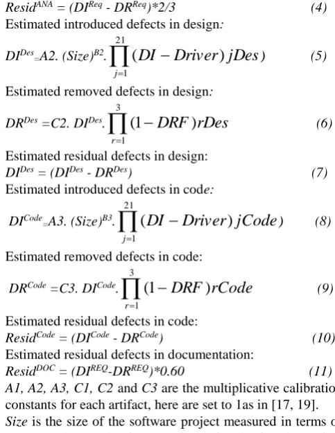
According to example fig 7, the following equations estimate introduced, removed and residual defects in each task/ activity at each mode based on the cost in that mode. Estimated introduced defects in requirements:
DIReq
= A1. (Size)B1.
21
1
Re
)
(
j
q
j
Driver
DI
) (1)Estimated removed defects in requirements:
DRReq = C1. DIReq.
3
1
Re
)
1
(
r
q
r
DRF
(2)Estimated residual defects in Feasibility study:
ResidFS = (DIReq-DRReq)*1/3 (3)
Estimated residual defects in analysis:
ResidANA = (DIReq - DRReq)*2/3 (4)
Estimated introduced defects in design:
DIDes
=A2. (Size)B2.
21
1
)
(
j
jDes
Driver
DI
) (5)Estimated removed defects in design:
DRDes =C2. DIDes.
3
1
)
1
(
r
rDes
DRF
(6)Estimated residual defects in design:
DIDes = (DIDes - DRDes) (7)
Estimated introduced defects in code:
DICode
=A3. (Size)B3.
21
1
)
(
j
jCode
Driver
DI
) (8)Estimated removed defects in code:
DRCode =C3. DICode.
3
1
)
1
(
r
rCode
DRF
(9)Estimated residual defects in code:
ResidCode = (DICode - DRCode) (10)
Estimated residual defects in documentation:
ResidDOC = (DIREQ-DRREQ)*0.60 (11)
A1, A2, A3, C1, C2 and C3 are the multiplicative calibration constants for each artifact, here are set to 1as in [17, 19].
Size is the size of the software project measured in terms of KSLOC (thousands of source lines of code, function points or any other unit of size), here KSLOC is used as software size measure.
B1, B2 and B3 accounts for economies / diseconomies of scale and are initially set to 1 as in [17, 20].
(DI-driver)jReq , (DI-driver)jDes and (DI-driver)jCode are the Defect Introduction Driver for each artifact and the jth
factor.
r = 1 to 3 for each DR profile, namely automated analysis, people reviews, execution testing and tools
DRFrReq, DRFrDes andDRFrCode are Defect Removal Fraction
for defect removal profile r and artifact type (Req, Des and Code).
The flowchart, fig 4, shows how task quality in
each
mode
is
estimated.
Task cost in specific mode
Check task cost level i.e. VL or L, etc.
Determine ID driver's levels and removal profiles levels based on task cost level.
COQUAMO
Residual task defects in the mode Software
[image:4.595.61.293.44.609.2]size
[image:4.595.301.543.51.364.2]B. DTCQTP Representation and Assumptions
PDBO algorithm assumes that the DTCQTP has the representation of activity-on-node network and also assumes that every node (activity) in a network has virtual edges to all its modes as in fig 5. Activities 1 and 5 have virtual edges to all their modes where M1 is the first mode and Mn is last mode of an activity and the other activities have virtual edges to their modes similar to activities 1 and 5. Activities S and F don not have modes and therefore do not have virtual edges to modes because these are dummy activities.
C. Mathematical Modeling
The following notations are used to describe the DTCQTP: Ct: Total cost of project (direct plus indirect), Tt: Total duration of project, Qt: Total quality of project, Ic: Project indirect cost per time unit, Modes(i): Set of available execution modes for activity i, Cik: Direct cost of activity i
when performed the kth execution mode, tik: Duration of activity i when performed the kth execution mode, qik: Quality of activity i when performed the kth execution mode, yik: Binary variable which is 1 when mode k is assigned to activity i and 0 otherwise, Defects_Allowed: Upper bound for Project quality. Tcpm : Critical path duration obtained by critical bath method(CPM), if set of modes K = {k1,k2,….,kn}are assigned to activities;
Mixed integer programming is used for modeling DTCQTP:
Min Ct=
1
0 N
i
Modes(i)
k Cik .yik+ Ic . Tcpm (12)
Min Tt = Tcpm (13)
Subject to:
1
0 N
i
Modes(i)
k qik.yik <=Defects_Allowed (14)
kModes(i) yik=1. (15)yik
{0,1}
i,k (16)Objective functions (1) and (2) minimize the project's total costs and duration respectively. Constrain (3) enforces that the total quality of project does not bypass the desired level (upper bound). In (4) one and only one execution mode is assigned to each activity and equation (5) is sign constrains.
D. Problem Data Based Optimization (PDBO)
Algorithm
PDBO algorithm is a single agent meta-heuristic algorithm that depends on possibility calculated from problem's data. PDBO assumes the problem is represented in the form of a graph G = (V, E), in which the set of nodes
V represents the activities and modes, and the set of E
represents edges that connects between activities and modes. For optimization problems, at each iteration, PDBO selects the first node ni then depending on the best possibility
values, it moves to the next adjacent node nk. After then, in
order to increase the chance of selecting other nodes rather than node nk in the next iteration, PDBO technique updates
the Possibility(ni,nk) to be
Npossibility(ni,nk)=Possibility(ni,nk)+(cost/α) where α>0.
finally, after the best iteration solution found, in order to evaporate the Npossibilities, PDBO considers the parameter
β
[0.1], such that Npossibility(ni,nk)= Npossibility(ni,nk) –β, where β is the evaporation rate (reduction rate) of
Npossibility(ni,nk) for virtual edge between ni and nk.
PDBO manipulates the DTCQTP in the form of graph, in which the activities considered as nodes and the modes considered as virtual nodes connected to the activities through virtual edges fig 5. Possibility is calculated from problem's data (costs of activities). The PDBOalgorithm for DTCQTP is shown in fig 7.
VI. EXAMPLE
[image:5.595.304.546.359.597.2]Example with five task software programming project is considered fig 6, where activity 1 represents feasibility study and 2, 3, 4 and 5 represent requirements analysis, design, and code, documentation activities respectively and S and F are dummy activities. If bids offered from different subcontractors to perform specific activities in this project or this project will be developed in house, the modes take the forms as in table II below where task quality in each mode is estimated by COQUAMO and estimated software size is 25000 SLOC. In some large projects, many bids offered from many subcontractors to perform specific activities or tasks.
Fig. 5. DTCQTPrepresentation
Fig. 6. Project example
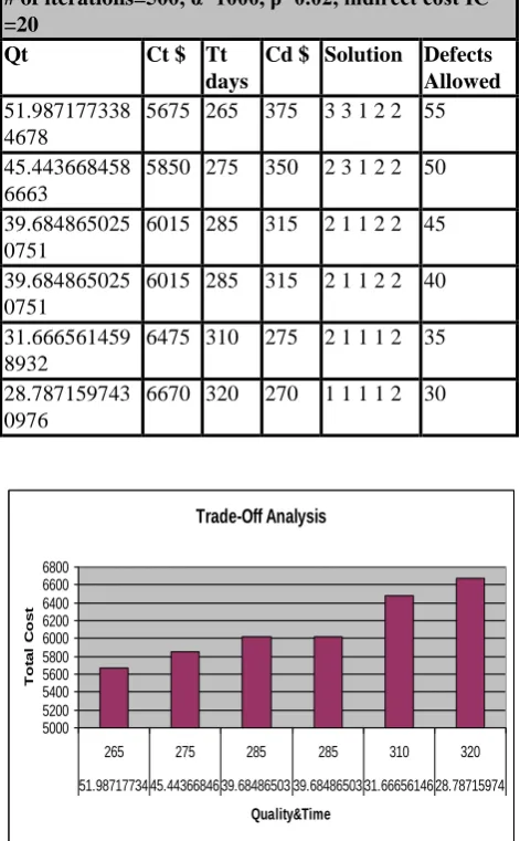
PDBO algorithm is implemented in c# and is tested and evaluated on CPU (Core( i5) 3210 M, 2.50 GHz) and 4GB RAM using Windows 7 as the operating system. Table III shows the results in terms of total quality Qt, cost Ct and time Tt with Direct cost Cd of applying PDBO to this project using different quality
bounds (Defects_Allowed). This project has about 54
solutions. The parameters of PDBO and direct costs are included in the first row of table III. From table III and fig 8, the total cost and time are increased by minimizing quality bounds (minimizing defects) which mean maximizing project quality. Fig 9 shows the processing time PT taken by PDBO algorithm to reach the solutions under different quality bounds.
S
2
1
3
F
4
5
M1
Mn
M1
Mn
S
2
1
3
F
4
TABLE II:EXECUTION MODES OF ACTIVITIES
TABLE III:FINAL OUTPUT OF PROGRAM
Trade-Off Analysis
5000 5200 5400 5600 5800 6000 6200 6400 6600 6800
265 275 285 285 310 320
51.98717734 45.44366846 39.68486503 39.68486503 31.66656146 28.78715974
Quality&Time
To
ta
l
C
os
[image:6.595.57.393.42.729.2]t
Fig. 8. Time-cost-quality trade-off analysis
Processing Time
00:00.0 00:00.0 00:00.0 00:00.0 00:00.0 00:00.0 00:00.0 00:00.0 00:00.0
55 50 45 40 35 30
Qualty bounds(defects_Allowed)
[image:6.595.305.551.53.173.2]PT
Fig. 9. Processingtime(PT)
1. Set parameters α, β and read problem data
2. Calculate Possibility(acti,modk) from problem data ,
i=1,..,Nc, k=1,…,Modes(acti).
3. While (termination condition not met) do 4. For each activity acti
5. Choose a mode modk of activity acti in
TCQTP with Minimum Possibilit. 6. Update possibility of virtual edge between
acti and chosen mode modk by
Possibility(acti,modk)=
Possibility (acti,modk)+ c(acti,modk)/α..
7. End i for
8. Find iteration solution
9. Evaporate a possibilities of virtual edges e(acti,modk)
between all activities and their chosen modes at this iteration by Possibility(acti,modk)=
Possibility (acti,modk) - β.
10. Update a total solution
11. Evaporate possibilities of virtual edges e(acti,modk)
that represent a total solution if no iteration solution exist by Possibility(acti,modk)=
Possibility (acti,modk)- β.
12. End while
[image:6.595.43.281.70.468.2]13. Return a total solution
Fig. 7. PDBO Algorithm for DTCQTP
VII. CONCLUTION AND DISCUSSION
In this paper, task quality in each mode is estimated by COQUAMO and thus a total number of residual defects for all tasks in chosen modes reflect the quality of the software project quantitatively.
In DTCQTP, each project task/activity can be executed in one of several modes. The execution modes of any activity were assumed to be bids offered from different subcontractors to perform specific tasks or different approaches can be used to perform the tasks if the software project will be developed in house.
Solving the problem gave an optimal/nearly optimal solution in terms of time, cost, and quality of the project. By changing the allowable quality bound for the project and re-running the algorithm, other optimal /nearly optimal solutions could be obtained. Having these optimal/nearly optimal solutions and analyzing the environments needs, project managers could make decisions effectively.
To solve the problem, PDBO algorithmwas introduced, which takes much less time to reach the optimal/nearly optimal solution under the allowable quality bound.
Activity number
Modes Cost in $
Time in days
Estimated Defects
1 1 60 100 2.7
2 65 80 5.57940171679557
3 90 70 12.1229105965972
2 1 45 90 5.4
2 55 90 5.4
3 80 65 11.1588034335911
4 100 45 24.2458211931943
3 1 80 70 18.13635349479
2 100 100 29.338849081258
4 1 35 100 2.06480624830767
2 75 75 10.0831098134896
3 95 100 15.665911985617
4 100 80 15.665911985617
5 1 65 75 1.0042923090232
2 50 50 0.486
3 75 60 1.0042923090232
# of iterations=500, α=1000, β=0.02, indirect cost IC =20
Qt Ct $ Tt
days
Cd $ Solution Defects Allowed 51.987177338
4678
5675 265 375 3 3 1 2 2 55
45.443668458 6663
5850 275 350 2 3 1 2 2 50
39.684865025 0751
6015 285 315 2 1 1 2 2 45
39.684865025 0751
6015 285 315 2 1 1 2 2 40
31.666561459 8932
6475 310 275 2 1 1 1 2 35
28.787159743 0976
[image:6.595.45.281.346.727.2]To achieve accurate estimation of task quality, COQUAMO need to be calibrated to origination database. In future work, we enhance COQUAMO accuracy by PDBO algorithm or another meta heuristic algorithm using NASA database.
REFERENCES
[1] Maryam Rahimi and Hossein Iranmanesh, “Multi Objective Particle Swarm Optimization for a Discrete Time, Cost and Quality Trade -off Problem”, World Applied Sciences Journal, vol.4, no.2, pp.270-276, 2008.
[2] N.S. Pour, M. Modarres, M.B. Aryanejad, R.T. Moghadam, “The Discrete Time-Cost-Quality Trade-off Problem Using a Novel Hybrid Genetic Algorithm”, Applied Mathematical Sciences, Vol. 4, no. 42, pp. 2081 – 2094, 2010.
[3] N.S. Pour, M. Modarres and R.T. Moghaddam, “Time-Cost-Quality Trade-off in Project Scheduling with Linguistic Variables”, World Applied Sciences Journal 18 (3): 404-413, 2012.
[4] [4] H.R. Tarighian and S.H. Taheri, “on the discrete time, cost and quality trade-off problem”, Applied Mathematics and Computation 181 (2006), 1305–1312.
[5] R.H, A. El Razek, A.M. Diab, S.M. Hafez, R.F. Aziz, “Time-Cost-Quality Trade-off Software by using Simplified Genetic Algorithm for Typical repetitive Construction Projects”, World Academy of Science, Engineering and Technology, 37, 2010.
[6] N.R Shankar, M.M.K.. Raju, G. Srikanth, P.H. Bindu, “Time, Cost and Quality Trade-off Analysis in Construction of Projects”, Contemporary Engineering Sciences, Vol. 4, no. 6, pp.289 – 299, 2011.
[7] H. Iranmanesh, M.R. Skandari, M. Allahverdiloo, “Finding Pareto Optimal Front for the Multi-Mode Time, Cost Quality Trade-off in Project Scheduling”, World Academy of Science, Engineering and Technology 40 2008.
[8] A. Afshar, A. Kaveh, O.R. Shoghli, “Multi-objective optimization of time-cost-quality using multi-colony ant algorithm”, Asian Journal of Civil Engineering (building and housing), vol. 8, NO. 2 (2007), Pages 113-124.
[9] E. Demeulemeester, B. De Reyck, B. Foubert, W. Herroelen ,M. Vanhoucke, “New computational results on the discrete time/cost trade-off problem in project networks” , Journal of the Operational Research Society (1998) 49, 1153-1163
[10] Ahmed Baykal Hafizoglu, “Discrete time/cost tradeoff problem in project scheduling,”, a thesis submitted to the graduate school of natural and applied sciences of Middle East technical university, June 2007.
[11] M.H. Rasmy, H.M.E. Abdelsalam, R.R. Hussein, “Multi-Objective Time-Cost Trade-Off Analysis in Critical Chain Project Networks Using Pareto Simulated Annealing, ”, Faculty of Computers & Information-Cairo University, March 2008.
[12] Amin Zeinalzadeh, “An Application of Mathematical Model to Time-cost Trade off Problem (Case Study) ”, Australian Journal of Basic and Applied Sciences, pp. 208-214, 2011.
[13] Do Ba Khang and Yin Mon Myint, “Time, cost and quality trade-off in project management: a case study”, International Journal of Project Management, Vol. 17, No. 4, pp. 249-256, 1999.
[14] R.M. Ahari and S.T. A. Niaki, “Fuzzy Optimization in Cost, Time and Quality Trade-off in Software Projects with Quality Obtained by Fuzzy Rule Base”, International Journal of Modeling and Optimization, Vol. 3, No. 2, April 2013.
[15] Babu and Suresh, “Project management with time, cost and quality considerations”, European Journal of Operational research, pp. 320-327, 1996.
[16] Ian Sommerville, “software engineering”, ninth edition, Addison-Wesley, 2011.
[17] Sunita Chulani, “results of Delphi for the defects introduction model (sub-model of the cost/quality model extension to COCOMO II) ”, Center for software engineering, 1997.
[18] David Chappell, “the three aspects of software quality: functional, structural, and process”, available at http://www.davidchappell.com/writing/white_papers/The_Three_Asp ects_of_Software_Quality_v1.0-Chappell.pdf (cited 9.11.2014). [19] Sunita Chulani and Barry Boehm, “Modeling Software Defect
Introduction and Removal: COQUALMO (Constructive Quality Model) ”, USC - Center for Software Engineering, Los Angeles, CA 90089-0781, 1999.
[20] Capers Jones, “software defect origin and removal methods”, Draft 5.0 , December 28, 2012.