Mass assembly and morphological transformations since z∼ 3 from CANDELS

(1)

Advance Access publication 2016 July 30

Mass assembly and morphological transformations since

z

∼

3 from CANDELS

M. Huertas-Company,

1,2‹

M. Bernardi,

2

P. G. P´erez-Gonz´alez,

3

M. L. N. Ashby,

4

G. Barro,

5

C. Conselice,

6

E. Daddi,

7

A. Dekel,

8

P. Dimauro,

1

S. M. Faber,

9

N. A. Grogin,

10

J. S. Kartaltepe,

11

D. D. Kocevski,

12

A. M. Koekemoer,

10

D. C. Koo,

9

S. Mei

1,13

and F. Shankar

14

Affiliations are listed at the end of the paper

Accepted 2016 July 22. Received 2016 July 22; in original form 2016 May 2

A B S T R A C T

We quantify the evolution of the stellar mass functions (SMFs) of star-forming and

quies-cent galaxies as a function of morphology fromz∼3 to the present. Our sample consists

of ∼50 000 galaxies in the CANDELS fields (∼880 arcmin2_{), which we divide into four}

main morphological types, i.e. pure bulge-dominated systems, pure spiral disc-dominated,

intermediate two-component bulge+disc systems and irregular disturbed galaxies. Atz∼2,

80 per cent of the stellar mass density of star-forming galaxies is in irregular systems. However,

byz∼0.5, irregular objects only dominate at stellar masses below 109_M_{. A majority of}

the star-forming irregulars present atz∼2 undergo a gradual transformation from disturbed

to normal spiral disc morphologies by z∼ 1 without significant interruption to their star

formation. Rejuvenation after a quenching event does not seem to be common except perhaps for the most massive objects, because the fraction of bulge-dominated star-forming galaxies

withM∗/M>1010.7 reaches 40 per cent atz < 1. Quenching implies the presence of a

bulge: the abundance of massive red discs is negligible at all redshifts over 2 dex in stellar

mass. However, the dominant quenching mechanism evolves. Atz >2, the SMF of quiescent

galaxies aboveM∗is dominated by compact spheroids. Quenching at this early epoch destroys

the disc and produces a compact remnant unless the star-forming progenitors at even higher

redshifts are significantly more dense. At 1< z <2, the majority of newly quenched galaxies

are discs with a significant central bulge. This suggests that mass quenching at this epoch

starts from the inner parts and preserves the disc. Atz <1, the high-mass end of the passive

SMF is globally in place and the evolution mostly happens at stellar masses below 1010_M_.

These low-mass galaxies are compact, bulge-dominated systems, which were environmentally quenched: destruction of the disc through ram-pressure stripping is the likely process.

Key words: galaxies: abundances – galaxies: evolution – galaxies: high-redshift – galaxies: structure.

1 I N T R O D U C T I O N

Lying at the centres of dark matter potential wells, galaxies are the building blocks of our Universe. How they assemble their mass and acquire their morphology are two central open questions today. The answer requires a complete understanding of the complex baryonic physics which dominate at these scales. At first order, however, a galaxy is a system that transforms gas into stars. The life of a galaxy is therefore a balance between processes that trigger star formation

_E-mail:_{[email protected]}

by accelerating gas cooling and others which tend to prevent star formation by expelling or heating gas (e.g. Lilly et al.2013). Stellar mass functions (SMFs) are a key first-order observable which allows one to statistically trace back the formation of stars in the universe. Comparison with predicted SMFs constrains the mechanisms which trigger, enhance or inhibit star formation.

Deep NIR surveys over large areas undertaken in the last years probe the evolution of the SMFs fromz∼4 (e.g. P´erez-Gonz´alez et al.2008; Ilbert et al.2013; Muzzin et al.2013). They have shown that some form of feedback, to avoid the overformation of stars both at the high-mass and low-mass ends, is necessary. Another key result is that the abundance of passive galaxies steadily increases

at University of Nottingham on January 4, 2017

http://mnras.oxfordjournals.org/

(2)

times, there are more passive than star-forming galaxies with this mass, so mass quenching becomes less relevant. Therefore, at late times, most of the quenching activity happens below∼1010.7_M

, and this tends to flatten the low-mass end of the passive galaxy SMF (e.g. Moutard et al.2016). Since most of these galaxies are satellites, this quenching is generally referred to asenvironmental quenching. Even though this empirical description of quenching has been extremely successful in explaining the global trends, the actual physical mechanisms behind quenching are still largely un-constrained.

SMFs alone do not provide information on how the formation of stars affects galaxy structure. It is however well established that star formation activity is strongly correlated with morphol-ogy. Galaxies which live on the main sequence of star formation tend to have a disc-like morphology with low S´ersic indices, while passive galaxies tend to have early-type morphologies and S´ersic indices larger than 2 (e.g. Wuyts et al.2011). Whether this is a cause or a consequence is not yet known (Lilly & Carollo2016). Several studies claim that the observed relation between structure and star formation is in fact a consequence of very dissipative quenching processes. A large amount of gas would be driven into the central parts of the galaxies producing a central burst of star formation and therefore a bulge with high central stellar mass density (e.g. Barro et al.2013,2015). However, recent evidence suggests that the dom-inant quenching mechanism at intermediate stellar masses might be simply a shutting off of the gas supply through strangulation (e.g. Peng, Maiolino & Cochrane2015) without significant morphologi-cal transformations even at very high redshifts (e.g. Feldmann et al.

2016). The observed correlation between central stellar mass den-sity and star formation rate could be mostly explained by the fading of the disc after the strangulation event (e.g. Carollo et al.2014). This would also explain the relative large abundance of fast-rotating passive galaxies in the local universe (see Cappellari2016for a re-view).

Properly quantifying how the joint distribution of morphology and mass evolves might shed new light on which are the main quenching processes. It also provides a new element of comparison with recent numerical and empirical simulations which now predict morphologies and structure (e.g. Vogelsberger et al.2014). How-ever, there is currently no benchmark measurement of this type. Large surveys such as SDSS (z≤0.25; Bernardi et al.2013) and more recently GAMA (z≤0.06; Moffett et al.2016) have enabled a good quantification of the morphological dependence of the SMF at low redshift (the larger volume of the SDSS means it is able to probe rarer higher masses than GAMA). Pushing to higher redshift requires better angular resolution over large areas. As a result, there are very few complete studies of the morphological dependence of the SMF at high redshift. Bundy, Ellis & Conselice (2005) made a

ferent morphologies in the early universe. This is the main purpose of the present work.

In Huertas-Company et al. (2015), we used new deep-learning techniques to estimate the morphologies of all galaxies withH<

24.5 in the five CANDELS fields with unprecedented accuracy.1 We now use these morphologies, together with robust stellar mass estimates from extensive multi-band imaging, to study the evolu-tion of the SMFs of quiescent and star-forming galaxies of different morphologies fromz∼3, for the first time. We then discuss the im-plications for the dominant quenching processes and morphological transformations. The data on the mass functions are made public so that they can be directly compared with the predictions of different models.

The paper is organized as follows. In Section 2, we describe the data set used as well as the main physical parameters we mea-sure (morphologies, structural parameters, stellar masses, etc.). In Section 3, we describe the methodology used to derive the SMFs. Section 4 discusses their evolution. Finally in Section 5, we discuss the implications for the star formation histories (SFHs) of the differ-ent morphologies and the evolution of the quenching mechanisms at different cosmic epochs.

Throughout the paper, we assume a flat cosmology withM= 0.3,=0.7 andH0=70 km s−1Mpc−1and we use magnitudes in the AB system. All stellar masses were scaled to a Chabrier (2003) initial mass function (IMF).

2 DATA S E T

2.1 Parent sample

Galaxies in the five CANDELS fields (UDS, COSMOS, EGS, GOODS-S, GOODS-N) are selected in theF160Wby applying a magnitude cutF160W<24.5 mag (AB). The total area is∼880 arcmin2_{. We use the CANDELS public photometric catalogues for} UDS (Galametz et al.2013) and GOODS-S (Guo et al.2013) and soon-to-be-published CANDELS catalogues for COSMOS, EGS (Stefanon et al., in preparation) and GOODS-N (Barro et al., in preparation). The magnitude cut is required to ensure that the avail-ability of morphologies (Huertas-Company et al.2015) a key quan-tity for the analysis presented in this work. The stellar mass com-pleteness resulting from this magnitude cut is extensively discussed in Section 2.4 given its importance to derive reliable SMFs.

1_{The catalogue is available at} _{http://rainbowx.fis.ucm.es/Rainbow_}

navigator_public/.

(3)

2.2 Structural properties

We use the publicly available 2D single S´ersic fits from van der Wel et al. (2012) to estimate basic structural parameters (radii, S´ersic indices, axial ratios). The fist were done usingGALFIT(Peng et al.

2002) on the three NIR images (F105W, F125W, F160W). The expected uncertainty on the main parameters is less than 20 per cent for the magnitude cut applied in this work as widely discussed in van der Wel et al. (2012,2014).

2.3 Morphological classification

We use the deep-learning morphology catalogue described in Huertas-Company et al. (2015). In brief, the ConvNets-based al-gorithm is trained with visual morphologies available in GOODS-S and then applied to the remaining four fields. Following the CAN-DELS classification scheme, we assign five numbers to each galaxy:

fsph,fdisc,firr,fPS,fUnc. These measure the frequency with which hy-pothetical classifiers would have flagged the galaxy as having a spheroid, a disc, presenting an irregularity, being compact (or a point source) and being unclassifiable/unclear. For a given image, ConvNets are able to predict the variousftypevalues with negligible bias on average, scatter of∼10 per cent–15 per cent, and fewer than 1 per cent misclassifications (Huertas-Company et al.2015).

In what follows, we primarily use theHband (F160W) since our sample is dominated by galaxies atz >1, where NIR filters probe the optical rest frame. Forz <1 galaxies, we also explored the

I-band filters (814W, 850LP) but because the classes we define below are quite broad, the classifications do not change significantly (also see Kartaltepe et al.2015). In addition, as we show below, at low redshifts our classifications match those in the SDSS rather well: morphologicalk-corrections do not have a big impact on our results. In this work, we distinguish four main morphological types de-fined as follows:

(i)spheroids [SPH]: fsph>2/3 andfdisc<2/3 andfirr<0.1 (ii)late-type discs [DISC]: fsph<2/3 andfdisc>2/3 andfirr< 0.1

(iii)early-type discs [DISCSPH]: fsph>2/3 andfdisc>2/3 and

firr<0.1

(iv)irregulars [IRR]: fsph<2/3 andfirr>0.1.

The thresholds above are somewhat arbitrary but have been cali-brated through visual inspection first to make sure that they indeed result in distinct morphological classes (see also Kartaltepe et al.

2014).

In Appendix A, we show some randomly selected postage stamps of the different morphological classes in the COSMOS/CANDELS field sorted by stellar mass and redshift. Slight changes to the thresh-olds used to define these classes do not affect our main results. The SPH class contains bulge-dominated galaxies with little or no disc: it should be close to the classical elliptical classification used in the local universe. The DISC class is made of galaxies in which the disc component dominates over the bulge (typically Sb-c galaxies). Between both classes lies the DISCSPH class in which there is no clear dominant component: it should include typical S0 galaxies and early-type spirals (Sa). We also distinguish galaxies with clear asymmetry in their light profiles. This category should capture the variety of irregular systems usually observed in the high-redshift universe (e..g clumpy, chain, tadpole, etc.). This irregular class might contain a wide variety of galaxies with different physical properties since the classification is based on the irregularity of the light profile. Notice thatIRRis defined with no condition onfdisc;

therefore, this class can include many late-type discs at low redshifts (i.e. Sds).

We have verified that the different classes have distinct structural properties. Spheroids are more compact, rounder (b/a∼0.8) and have larger Sérsic indices (n∼4–5) than all other morphologies at all stellar masses and at all redshifts. On the other extreme, discs are larger, more elongated (b/a∼0.5) and have Sérsic indices close to 1, as expected. Disc+spheroids systems lie somewhat in between: they have Sérsic indices∼2, but are less compact than the spheroids and have similar axial ratios to discs (in agreement with the visual classification; also see Huertas-Company et al.2015). Although a detailed analysis of the structural properties of the different mor-phologies will be presented elsewhere, Appendix B shows that the different morphologies also have different stellar mass bulge-to-total ratios (B/Ts).

2.4 Stellar masses and completeness

Spectral Energy Distribution (SED) fitting is used to estimate pho-tometric redshifts and stellar masses used in this work. The detailed methodology is described in Wuyts et al. (2011,2012) and Barro et al. (2013,2014). Therefore, only the main points are discussed here. Photometric redshifts are the result of combining different codes to improve the individual performance. The technique is fully described in Dahlen et al. (2013). Based on the best avail-able redshifts (spectroscopic or photometric), we then estimate stellar mass-to-light ratios from the PEGASE01 models (Fioc & Rocca-Volmerange1999). For these, we assume solar metallicity, exponentially declining SFHs, a Calzetti et al. (2000) extinction law and a Salpeter (1955) IMF. TheM∗/Lvalues are then converted to a Chabrier IMF by applying a constant 0.22 dex shift. The stellar mass is estimated by multiplying theM∗/Lvalue by the S´ersic-basedL(fromGALFIT2D fits – see Section 2.2). See also Bernardi et al. (2013, Bernardi et al.2016) for extensive discussion of the systematics associated with all these choices.

The stellar mass completeness of the sample is estimated fol-lowing the methodology of Pozzetti et al. (2010) and Ilbert et al. (2013) separately for star-forming and quiescent galaxies. We first compute the lowest stellar mass (Mlim∗ ) which could be observed for each galaxy of magnitudeHgiven the applied magnitude cut (H<24.5): log(Mlim∗ )=log(M∗)+0.4(H−24.5). We then esti-mate the completeness as the 90th percentile of the distribution of

Mlim, i.e. the stellar mass for which 90 per cent of the galaxies have lower limiting stellar masses. By adopting this threshold, we make sure that at most 10 per cent of the low-mass galaxies are lost in each redshift bin. Fig.1shows the distribution of galaxies in our sample in the mass–redshift plane and the adopted stellar mass com-pleteness as a function of redshift for passive and all galaxies. The sample is roughly complete for galaxies above 1010 _{solar masses} atz∼3 and goes down to 109_at_z_∼_{0.5 (see also Table}₁_{). As a} sanity check, we use an alternative estimate of the stellar mass com-pleteness by taking advantage of the fact that the CANDELS data are significantly deeper than theH-band selected sample used here (H<24.5). We therefore compute in bins of redshift the stellar mass at which 90 per cent of the galaxies in the full CANDELS catalogue are also included in our bright selection. The resulting stellar mass completeness is overplotted in Fig. 1. It agrees reasonably well with the one estimated independently using the methodology by Pozzetti et al. (2010). The largest differences are observed at the high-mass end. It can be a consequence of low statistics in these stellar mass bins. In the following, we will adopt therefore the first

(4)

[image:4.595.90.501.55.253.2]

Figure 1. Stellar mass as a function of redshift for all galaxies (left-hand panel) and quiescent galaxies (right-hand panel) for ourH<24.5 selected sample. Blue points show the minimum stellar mass which can be observed for a given galaxy computed as explained in the main text. The red line shows the 90th percentile of the distribution ofMlimwhich is the adopted mass completeness in this work (see the text for details). The orange line shows the mass completeness

estimated using the full-depth CANDELS catalogue (see the text for details).

estimate, keeping in mind however that at high redshift we might underestimate the completeness.

2.5 Quiescent/star-forming separation

Rest-frame magnitudes (U,Vand J) are computed based on the best-fitting redshifts and stellar templates (see Section 2.4) and are then used to separate the passive and star-forming populations as widely used in the previous literature (Whitaker et al.2012). This colour–colour separation has the advantage of properly distinguish-ing galaxies reddened by dust from real passive galaxies with old stellar populations.

3 E S T I M AT I O N O F M O R P H O L O G I C A L S M F s

We use theVmaxestimator (Schmidt1968) to derive the SMFs in this work. It has the advantage of being very simple but can easily diverge when the incompleteness becomes too important. For this reason, we restrict our analysis to stellar masses above the thresholds derived in Section 2.4 and quoted in Table1. Recent works have shown that above the completeness limits, very consistent results are obtained with maximum-likelihood methods (e.g. Ilbert et al.

2013). For simplicity, we restrict our analysis to one single estimator throughout this work.

3.1 Uncertainties

We consider three sources of errors which contribute to the uncer-tainties on the SMFs. Namely Poisson errors (σP), cosmic variance (σCV) and errors associated with the estimation of stellar masses and photometric redshifts (σT). Poisson errors reflect exclusively statistical uncertainties due to the limited number of galaxies in each bin. They are proportional to the square root of the number of objects. Cosmic variance errors are related to the fact that we observe a small area in the sky so our measurements can be affected by statistical fluctuations in the number of galaxies due to the un-derlying large-scale density fluctuations. Cosmic variance can be computed from the galaxy bias and the dark matter cosmic variance

assuming a cold dark matter (CDM) model. We use the tool of Moster et al. (2011) to estimate the fractional error in density given the size of the CANDELS fields and also their spatial distribution. Finally, uncertainties in stellar mass and redshifts do have an impact on the density of galaxies. Stellar masses are obtained through SED fitting assuming a photometric redshift (spectroscopic redshifts are available for a minority of sources). There are therefore systematic (e.g. template errors, IMF assumptions, SFHs) and statistical errors associated with this methodology.

To estimate this uncertainty, we take advantage of the various measurements of stellar masses and redshifts existing in CAN-DELS. For example the 3D-HST team has computed an indepen-dent set of photometric redshifts and derived stellar masses using theFASTandEAZYcodes (Skelton et al.2014). They used Bruzual & Charlot (2003, hereafterBC03) models and a Chabrier IMF. A comparison of the two should provide an estimate of the errors in-duced in the SMFs due to errors in redshifts and stellar masses. We therefore generated a set of 50 catalogues by randomly combining stellar masses and photometric redshifts from the CANDELS and 3D-HST catalogues and recomputed the SMFs for each of them. We then measured the scatter in the final 50 SMFs in bins of redshift and stellar mass. This scatter combines the statistical error associated with estimatingM_∗from fitting noisy photometry to a given set of templates, with the systematic error associated with the fact that the templates used have built-in assumptions about the SFH (bursty or not? dusty or not?, etc.). We note however that this approach cer-tainly underestimates the errors. There is in fact a large overlap in assumptions made, notably the exponentially declining tau models and Calzetti reddening law. Additionally, although the photometric extractions by the 3D-HST and CANDELS teams were done in-dependently, the actual data on which the photometry is based are nearly identical. This is clearly not ideal. Nevertheless, we lump these together and add in quadrature to the other two terms. Hence, to each bin we assign an uncertainty

σ =σ2 P+σ

2 CV+σ

2 T.

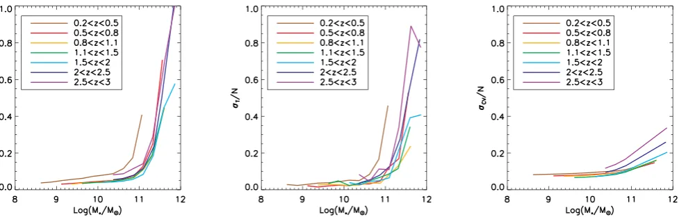
Fig.2shows the different fractional errors on the number density of galaxies as a function of stellar mass and redshift for the total

(5)

[image:5.595.57.545.82.570.2]

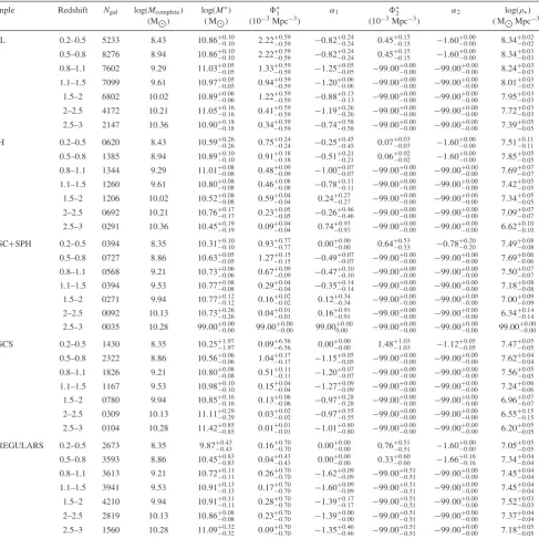
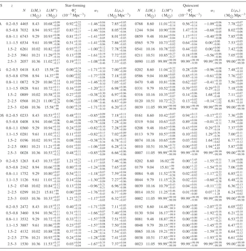
Table 1. Best-fitting parameters with single and double Schechter functions to the SMFs of the four morphological types defined in this work. The parameters of the double Schechter are set to−99 whenever a single Schechter was used. Values of−99 are also used when the fit did not converge.

Sample Redshift Ngal log(Mcomplete) log(M∗) ∗1 α1 ∗2 α2 log(ρ∗)

(M) ( M) (10−3_Mpc−3₎ ₍₁₀−3_Mpc−3₎ _{( M}

Mpc−3₎

ALL 0.2–0.5 5233 8.43 10.86₋+₀0._.10₁₀ 2.22+₋0₀._.59₅₉ −0.82+₋0₀_..24₂₄ 0.45₋+0₀._.₁₅15 −1.60₋+0₀._.00₀₀ 8.34+₋0₀._.02₀₂ 0.5–0.8 8276 8.94 10.86+₋0₀._.10₁₀ 2.22+₋0₀._.59₅₉ −0.82+₋0₀_..24₂₄ 0.45₋+0₀._.₁₅15 −1.60₋+0₀._.00₀₀ 8.34+₋0₀._.03₀₃ 0.8–1.1 7602 9.29 11.03+₋0₀._.₀₅05 1.33₋+0₀._.59₅₉ −1.25+₋0₀._.₀₅05 −99.00₋+₀0._.00₀₀ −99.00₋+₀0._.00₀₀ 8.24+₋0₀._.03₀₃ 1.1–1.5 7099 9.61 10.97+₋₀0_..05₀₅ 0.94₋+0₀_..59₅₉ −1.20₋+00..0606 −99.00+

0.00

−0.00 −99.00+ 0.00

−0.00 8.01+ 0.03 −0.03

1.5–2 6802 10.02 10.89+₋0₀._.₀₆06 1.22₋+0₀._.59₅₉ −0.88+₋0₀._.₁₃13 −99.00₋+₀0._.00₀₀ −99.00₋+₀0._.00₀₀ 7.95+₋0₀._.03₀₃ 2–2.5 4172 10.21 11.05+₋0₀._.₁₆16 0.41₋+0₀._.59₅₉ −1.19+₋0₀._.₂₆26 −99.00₋+₀0._.00₀₀ −99.00₋+₀0._.00₀₀ 7.72+₋0₀._.03₀₃ 2.5–3 2147 10.36 10.90+₋0₀._.₁₈18 0.34₋+0₀._.59₅₉ −0.74+₋0₀._.₅₈58 −99.00₋+₀0._.00₀₀ −99.00₋+₀0._.00₀₀ 7.39+₋0₀._.05₀₅ SPH 0.2–0.5 0620 8.43 10.59₋+₀0._.26₂₆ 0.75+₋0₀._.24₂₄ −0.25+₋0₀_..45₄₅ 0.07₋+0₀._.₀₃03 −1.60₋+0₀._.00₀₀ 7.51+₋0₀._.11₁₁ 0.5–0.8 1385 8.94 10.89+₋0₀._.10₁₀ 0.91+₋0₀._.18₁₈ −0.51+₋0₀_..21₂₁ 0.06₋+0₀._.₀₂02 −1.60₋+0₀._.00₀₀ 7.85+₋0₀._.05₀₅ 0.8–1.1 1344 9.29 11.01+₋0₀._.₀₈08 0.48₋+0₀._.09₀₉ −1.00+₋0₀._.₀₇07 −99.00₋+₀0._.00₀₀ −99.00₋+₀0._.00₀₀ 7.69+₋0₀._.07₀₇ 1.1–1.5 1260 9.61 10.80+₋0₀._.₀₈08 0.46₋+0₀._.08₀₈ −0.78+₋0₀._.₁₁11 −99.00₋+₀0._.00₀₀ −99.00₋+₀0._.00₀₀ 7.42+₋0₀._.05₀₅ 1.5–2 1206 10.02 10.52+₋0₀._.₀₈08 0.59₋+0₀._.04₀₄ 0.24+₋0₀._.₂₇27 −99.00₋+₀0._.00₀₀ −99.00₋+₀0._.00₀₀ 7.34+₋0₀._.05₀₅ 2–2.5 0692 10.21 10.76+₋0₀._.₁₇17 0.23₋+0₀._.05₀₅ −0.26+₋0₀._.₄₆46 −99.00₋+₀0._.00₀₀ −99.00₋+₀0._.00₀₀ 7.09+₋0₀._.07₀₇ 2.5–3 0291 10.36 10.45+₋0₀._.₁₉19 0.09₋+0₀._.04₀₄ 0.74+₋0₀._.₉₃93 −99.00₋+₀0._.00₀₀ −99.00₋+₀0._.00₀₀ 6.62+₋0₀._.10₁₀ DISC+SPH 0.2–0.5 0394 8.35 10.31+₋0₀_..₁₀10 0.93₋+0₀._.77₇₇ 0.00+₋₀0_..00₀₀ 0.64₋+₀0._.53₅₃ −0.78+₋0₀._.20₂₀ 7.49+₋0₀._.08₀₈ 0.5–0.8 0727 8.86 10.63+₋0₀._.₀₅05 1.27₋+0₀._.15₁₅ −0.49+₋00..0707 −99.00−+00..0000 −99.00−+00..0000 7.69+−00..0606

0.8–1.1 0568 9.21 10.73+₋00..0606 0.67−+00..0909 −0.47+−00..1010 −99.00−+00..0000 −99.00−+00..0000 7.50+−00..0707

1.1–1.5 0394 9.53 10.77+₋0₀._.₀₈08 0.29₋+0₀._.04₀₄ −0.35+₋0₀._.₁₄14 −99.00₋+₀0._.00₀₀ −99.00₋+₀0._.00₀₀ 7.18+₋0₀._.08₀₈ 1.5–2 0271 9.94 10.77+₋0₀._.₁₂12 0.16₋+0₀._.02₀₂ 0.12+₋0₀._.₃₄34 −99.00₋+₀0._.00₀₀ −99.00₋+₀0._.00₀₀ 7.00+₋0₀._.09₀₉ 2–2.5 0092 10.13 10.73+₋0₀._.₂₆26 0.04₋+0₀._.01₀₁ 0.16+₋0₀._.₉₁91 −99.00₋+₀0._.00₀₀ −99.00₋+₀0._.00₀₀ 6.34+₋0₀._.14₁₄ 2.5–3 0035 10.28 99.00+₋0₀._.₀₀00 99.00₋+0₀._.00₀₀ 99.00+₀_.₀₀0.00 −99.00+₋0₀_..₀₀00 −99.00+₋₀0_..00₀₀ 99.00+₋0₀._.00₀₀ DISCS 0.2–0.5 1430 8.35 10.25+₋1₁._.97₉₇ 0.09+₋6₆._.56₅₆ 0.00+₋0₀_..00₀₀ 1.48₋+1₁._.₀₃03 −1.12₋+0₀._.05₀₅ 7.47+₋0₀._.05₀₅

0.5–0.8 2322 8.86 10.56+₋0₀._.₀₆06 1.04₋+0₀._.17₁₇ −1.15+₋0₀._.₀₅05 −99.00₋+₀0._.00₀₀ −99.00₋+₀0._.00₀₀ 7.62+₋0₀._.04₀₄ 0.8–1.1 1826 9.21 10.80+₋0₀._.₀₈08 0.51₋+0₀._.11₁₁ −1.20+₋0₀._.₀₇07 −99.00₋+₀0._.00₀₀ −99.00₋+₀0._.00₀₀ 7.56+₋0₀._.05₀₅ 1.1–1.5 1167 9.53 10.98+₋0₀._.₁₀10 0.15₋+0₀._.04₀₄ −1.27+₋0₀._.₀₉09 −99.00₋+₀0._.00₀₀ −99.00₋+₀0._.00₀₀ 7.24+₋0₀._.06₀₆ 1.5–2 0780 9.94 10.85+₋0₀._.₁₆16 0.13₋+0₀._.06₀₆ −0.97+₋0₀._.₂₈28 −99.00₋+₀0._.00₀₀ −99.00₋+₀0._.00₀₀ 6.96+₋0₀._.07₀₇ 2–2.5 0309 10.13 11.11+₋0₀._.₂₉29 0.03₋+0₀._.02₀₂ −0.97+₋0₀._.₅₅55 −99.00₋+₀0._.00₀₀ −99.00₋+₀0._.00₀₀ 6.55+₋0₀._.15₁₅ 2.5–3 0104 10.28 11.42+₋0₀._.₈₅85 0.01₋+0₀._.01₀₁ −1.01+₋0₀._.₈₀80 −99.00₋+₀0._.00₀₀ −99.00₋+₀0._.00₀₀ 6.20+₋0₀._.05₀₅ IRREGULARS 0.2–0.5 2673 8.35 9.87+₋00..4343 0.16+

0.70

−0.70 0.00+ 0.00

−0.00 0.76+ 0.51

−0.51 −1.60+ 0.00

−0.00 7.05+ 0.05 −0.05

0.5–0.8 3593 8.86 10.45+₋0₀._.₈₃83 0.04₋+0₀._.43₄₃ 0.00+₋0₀._.₀₀00 0.33₋+₀0._.60₆₀ −1.66₋+₀0._.16₁₆ 7.34+₋0₀._.04₀₄ 0.8–1.1 3613 9.21 10.72+₋0₀._.₁₁11 0.26₋+0₀._.70₇₀ −1.62+₋0₀._.₀₉09 −99.00₋+₀0._.51₅₁ −99.00₋+₀0._.00₀₀ 7.45+₋0₀._.04₀₄ 1.1–1.5 3941 9.53 10.91+₋00..1313 0.17+

0.70

−0.70 −1.60+ 0.09

−0.09 −99.00+ 0.51

−0.51 −99.00+ 0.00

−0.00 7.45+ 0.04 −0.04

1.5–2 4210 9.94 10.91+₋0₀._.₁₁11 0.28₋+0₀._.70₇₀ −1.39+₋0₀._.₁₇17 −99.00₋+₀0._.51₅₁ −99.00₋+₀0._.00₀₀ 7.52+₋0₀._.03₀₃ 2–2.5 2819 10.13 10.86+₋0₀._.₀₈08 0.23₋+0₀._.70₇₀ −1.39+₋0₀._.₀₀00 −99.00₋+₀0._.51₅₁ −99.00₋+₀0._.00₀₀ 7.37+₋0₀._.04₀₄ 2.5–3 1560 10.28 11.09+₋0₀._.₃₂32 0.09₋+0₀._.70₇₀ −1.35+₋0₀._.₄₆46 −99.00₋+₀0._.51₅₁ −99.00₋+₀0._.00₀₀ 7.18+₋0₀._.05₀₅

sample. Cosmic variance dominates the error budget for stellar masses below∼1011_{. It is in fact always greater than 10 per cent} while Poisson and template fitting errors are generally below

∼5 per cent. At larger stellar masses, the small number statistics generate an increase in the Poisson and template errors, which can exceed 50 per cent at the very highest masses. In the morphology divided samples, the number of objects is obviously reduced and therefore the statistical errors dominate over comic variance effects at all stellar masses. Similar trends are observed when the objects are separated into star-forming and quiescent samples.

3.2 Schechter function fits

The non-parametricVmax estimator is fitted with a Schechter or double Schechter model, depending on the sample. Given that our sample is not large, especially when it is divided into different morphological types, we preferentially use a single Schechter fit forz >0.8. Only in the lower redshift bins, where the SMFs reach lower stellar masses and an upturn is observed, do we adopt a double Schechter as done in previous works (Pozzetti et al.2010; Ilbert et al.2013; Muzzin et al.2013). In all cases, we only fit data points above the completeness limit to avoid biases related to the

(6)

[image:6.595.56.545.54.210.2]

Figure 2. Fractional errors on the number densities of galaxies as a function of stellar mass and redshift for the total sample used in this work. The left-, middle and right-hand columns show Poisson errors, template fitting-related errors and the effects of cosmic variance.

fact that the 1/Vmax estimator tends to underestimate the number densities beyond the completeness limits.

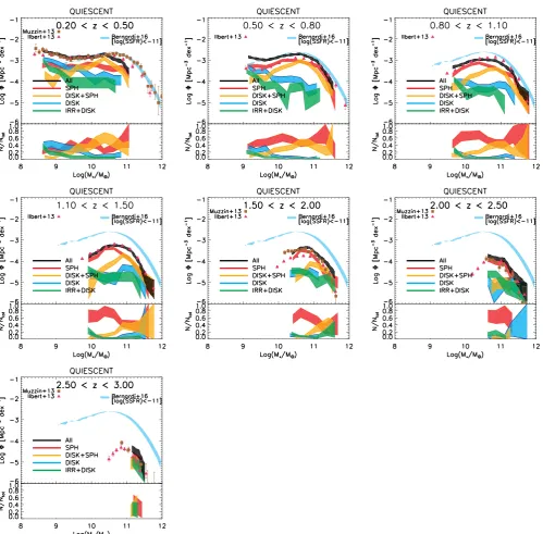
4 E VO L U T I O N O F T H E M O R P H O L O G I C A L S M F s

In this section, we discuss the evolution of the SMFs for different morphologies.

4.1 Full sample evolution

Fig.3shows the SMFs for each of the four morphological types defined previously; the different panels show results for seven red-shift bins. Fig.4shows the same information in a different format: each panel shows the evolution of the SMF for a fixed morpho-logical type. The redshift bin sizes were determined by a trade-off between number of objects and lookback time as seen in Tables1

and2. The functions are only plotted above the mass completeness limit derived in Section 2.4. Best-fitting parameters are shown in Table1.

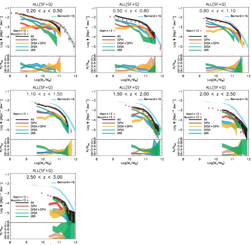
The global mass functions, i.e. not subdivided by morphology (black region in Fig. 3), are also shown and compared with re-cent measurements in the UltraVista survey by Ilbert et al. (2013) and Muzzin et al. (2013). There is good agreement despite the sig-nificantly smaller volume probed by the CANDELS fields. This suggests that our completeness limits are well estimated. Volume effects are mostly visible in the lowest redshift bin, where the CAN-DELS SMFs show a lack of very massive galaxies.

Before we consider CANDELS in more detail, it is worth re-marking on the cyan curve (same in each panel), which shows the SMF in the SDSS from Bernardi et al. (2016). The large volume of the SDSS means Poisson errors are negligible, so the shaded region encompasses the systematic differences between different

M∗/Lestimates. At lowz, the UltraVista measurements are in good agreement with the SDSS; moreover, they lie below it at higher red-shifts, as one might expect. In contrast, fig. 5 of Ilbert et al. (2013) shows that theirz∼0.5 SMF liesabovethez∼0.1 SDSS SMF, which does not make physical sense. This is because their fig. 5 used the SDSS estimate of Moustakas et al. (2013). Bernardi et al. (2016) discuss why their estimate is to be preferred; note that their work was not motivated by this problem, so the fact that evolution makes better physical sense when their SMF is used as the low-redshift benchmark provides additional support for their analysis. Very briefly, the main reason is that Moustakas et al. (2013) used

SDSS model magnitudes, which underestimate the total luminosity of bright galaxies (Bernardi et al.2010,2013; D’Souza, Vegetti & Kauffmann2015; see especially figs 2 and 3 in Bernardi et al.2016

and related discussion). This accounts for about half the difference from Bernardi et al.; the remainder is due toM_∗/L. Section 4.3 of Bernardi et al. (2016) discusses this in more detail (see, e.g., their figs 14–16). We refer the reader to Bernardi et al. (2016) for a more complete discussion.

If the evolution is driven by star formation (no mergers), then Fig.4shows that the stellar mass of galaxies belowM∗increases by more than 1 dex in the redshift range 0.5< z <3. More massive galaxies increase their stellar mass by less than 0.5 dex. Therefore, we confirm previous reports of a mass-dependent evolution for the global population. In addition, Table1shows that log(M∗/M)∼ 10.85±0.1 is approximately independent of redshift.

The key new ingredient of the present work is the evolution at fixed morphology. Morphological evolution and the mass depen-dence of the dominant morphology are both clearly observed. At 0.2 < z < 0.5, the population of ∼M∗ galaxies (10< log(M∗/M)<11) is essentially uniformly distributed between discs with low bulge fractions, spheroids with large B/Ts and inter-mediate objects with two components meaning that here is no clear dominant morphology at this mass scale. Above log(M_∗/M)= 11), objects with a clear bulge component tend to dominate the population. Below 1010_M

, the population is basically dominated by objects with small bulges or without. Irregular objects only start dominating the population at log(M∗/M)<9. This morphologi-cal distribution remains globally unchanged fromz∼1.

Our low-mass SMFs match the local SMFs recently derived in the GAMA survey (Moffet et al.2016) quite well, as shown in Fig.4. We overestimate the abundance of irregulars at log(M_∗/M)>10 compared to them. This is probably a consequence of our definition of irregulars based on the asymmetry of the light profile. It has how-ever little impact on the other morphologies since their abundance is still very low at the high-mass end. The agreement with their work confirms the robustness of our automated classifications.

Abovez∼1, irregular objects start dominating even at higher masses. Atz >2, the morphological mix changes radically: there are basically only two types of galaxies at these redshifts – irreg-ulars account for 70 per cent of the objects and bulge-dominated galaxies (spheroids) for the remaining 30 per cent (based on the extrapolations of the Schechter fits). This has a number of interest-ing implications. First, at these early epochs, the majority of discs are irregular (probably a signature of unstable discs as probed by

(7)

[image:7.595.49.548.54.541.2]

Figure 3. SMFs for four morphological types in different redshift bins as labelled. Red, blue, orange and green shaded regions in the top panels show the number densities of spheroids, discs, disc+spheroids and irregular/clumpy systems, respectively. The bottom panels show the fractions of each morphological type with the same colour code. The black regions show the global SMFs. The pink triangles and brown squares are the measurements by Ilbert et al. (2013) and Muzzin et al. (2013), respectively, in the UltraVista survey. The Muzzin et al. (2013) points are only plotted when their redshift bins are the same as the ones used in this work. We also show for reference in all panels the SMF for all SDSS galaxies (cyan shaded region) from Bernardi et al. (2016).

recent IFU surveys; e.g. Wisnioski et al.2015). Note that this is not a morphologicalk-correction effect, since we are probing the op-tical rest-frame band at this epoch. Secondly, symmetric discs and bulge+disc systems only begin to appear betweenz∼2 andz∼1; objects classified as DISC+SPH account for fewer than 5 per cent of the objects atz >2. This is also observed in the top-right panel of Fig.4. Discs and disc+spheroid mass functions experience the most dramatic evolution. One might worry that the apparent disap-pearance ofz≥2 discs is due to surface brightness dimming. This is unlikely though for several reasons. Extensive simulations (e.g.

van der Wel et al.2014; Kartaltepe et al.2015) have shown that discs should be detectable at the depth of the CANDELS survey for the magnitude selection used in this work. Also, these are fairly massive galaxies so there is not much room for the presence of a massive disc. In fact, preliminary results of Fig.B1show a clear correlation between the morphological classification and the stellar mass bulge-to-total ratio which would have been erased if surface brightness dimming was an issue.

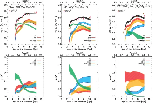
These global trends are captured in the top-left panel of Fig.5which summarizes the evolution of the stellar mass density

(8)

[image:8.595.313.507.50.489.2]

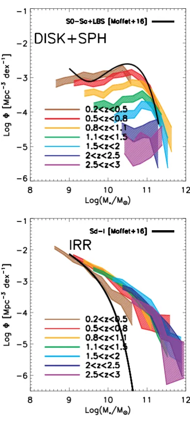
Figure 4. Evolution of the SMFs at fixed morphology. Same as Fig.3but binned by morphological type. Each colour shows a different redshift bin. We also overplot the local SMFs from Bernardi et al. (2016) for the total sample and the ones divided by morphology from Moffet et al. (2016) (best-fitting Schechter functions).

(9)

[image:9.595.49.547.100.609.2]

Table 2. Best-fitting parameters for a single Schechter function to the star-forming and quiescent SMFs of the four morphological types defined in this work. A=all, S=spheroids, D=discs, DS=discs+spheroids and I=irregulars. Quiescent galaxies atz >2.5 are not fitted because there are too few values above completeness. Quiescent irregulars are also very few. Although the fit works, the mass function is not always well described by a Schechter function. To emphasize this, we have set the error onM∗to 99.9.

S z Star-forming Quiescent

N L(Mc) L(M∗) ∗₁ α1 L(ρ∗) N L(Mc) L(M∗) ∗1 α1 L(ρ∗)

( M) ( M) (10−3_Mpc−3₎ _{( M}

Mpc−3₎ _{( M}

) ( M) (10−3_Mpc−3₎ _{( M}

Mpc−3₎

A 0.2–0.5 4465 8.43 10.68₋+0₀._.09₀₉ 0.92₋+0₀_..22₂₂ −1.46₋+₀0._.04₀₄ 7.85+₋0₀_..₀₅05 0768 8.60 11.01₋+₀0._.14₁₄ 0.56+₋0₀_..₁₄14 −1.09+₋0₀_..₀₆06 7.78+₋0₀._.07₀₇ 0.5–0.8 7032 8.94 10.92₋+0₀_..07₀₇ 0.83+₋0₀_..₁₇17 −1.46+₋0₀_..₀₄04 8.05+₋0₀._.04₀₄ 1244 9.04 10.90+₋0₀_..₀₄04 1.47+₋0₀._.16₁₆ −0.68+₋0₀._.05₀₅ 8.02+₋0₀._.06₀₆ 0.8–1.1 6743 9.29 10.93₋+0₀_..06₀₆ 0.81+₋0₀_..₁₇17 −1.41+₋0₀_..₀₅05 8.01+₋0₀._.03₀₃ 0859 9.48 10.84+₋0₀_..₀₄04 1.17+₋0₀._.11₁₁ −0.40+₋0₀._.08₀₈ 7.85+₋0₀._.06₀₆ 1.1–1.5 6534 9.61 10.98₋+₀0._.06₀₆ 0.51₋+0₀_..10₁₀ −1.41₋+₀0._.06₀₆ 7.86+₋0₀_..₀₃03 0565 9.79 10.73₋+0₀._.02₀₂ 0.64₋+0₀_..04₀₄ 0.00₋+0₀_..00₀₀ 7.53+₋0₀._.05₀₅

1.5–2 6261 10.02 10.82+₋0₀._.05₀₅ 0.93₋+0₀_..15₁₅ −1.00₋+00..1212 7.78+ 0.04

−0.04 0541 10.16 10.78+ 0.03 −0.03 0.44+

0.03

−0.03 0.00+ 0.00

−0.00 7.42+ 0.06 −0.06

2–2.5 3961 10.21 11.29+₋0₀_..₁₆16 0.13+₋0₀._.08₀₈ −1.61+₋0₀._.19₁₉ 7.72+₋0₀._.03₀₃ 0211 10.51 10.85+₋0₀._.27₂₇ 0.18+₋0₀._.08₀₈ −0.56+₋0₀._.86₈₆ 7.05+₋0₀._.08₀₈ 2.5–3 2057 10.36 11.02₋+0₀_..17₁₇ 0.19+₋0₀_..₁₁11 −1.08₋+0₀_..46₄₆ 7.33+₋₀0._.₀₅05 0090 11.05 99.99₋+99₉₉_..99₉₉ 99.99+₋₉99_.₉₉.99 99.99+₋99₉₉_..₉₉99 99.00+₋99₉₉._.99₉₉ S 0.2–0.5 0418 8.43 15.58+₋99₉₉ 0.00+₋0₀._.24₂₄ −1.71+₋0₀._.10₁₀ 7.00+₋0₀._.09₀₉ 0202 8.60 11.04+₋0₀._.22₂₂ 0.28+₋0₀._.09₀₉ −0.96+₋0₀._.08₀₈ 7.48+₋0₀._.10₁₀

0.5–0.8 0798 8.94 14.37+₋99₉₉ 0.00+₋0₀._.02₀₂ −1.77+₋0₀._.08₀₈ 7.18+₋0₀._.05₀₅ 0586 9.04 10.88+₋0₀._.05₀₅ 0.85+₋0₀._.10₁₀ −0.61+₋0₀._.06₀₆ 7.76+₋0₀._.07₀₇ 0.8–1.1 0872 9.29 10.86₋+0₀_..14₁₄ 0.10+₋0₀_..₀₄04 −1.46+₋0₀_..₁₀10 7.05+₋0₀._.07₀₇ 0470 9.48 10.81+₋0₀_..₀₆06 0.62+₋0₀._.07₀₇ −0.41+₋0₀._.10₁₀ 7.56+₋0₀._.09₀₉ 1.1–1.5 0928 9.61 10.72₋+₀0._.11₁₁ 0.16₋+0₀_..05₀₅ −1.20₋+₀0._.13₁₃ 6.98+₋0₀_..₀₆06 0331 9.79 10.52₋+0₀._.08₀₈ 0.39₋+0₀_..03₀₃ 0.29₋+0₀_..22₂₂ 7.18+₋0₀._.08₀₈ 1.5–2 0889 10.02 10.58₋+0₀_..10₁₀ 0.27+₋0₀_..₀₅05 −0.38₋+0₀_..30₃₀ 6.97+₋₀0._.₀₆06 0316 10.16 10.35₋+0₀_..07₀₇ 0.14+₋0₀_..₀₆06 1.68+₋0₀_..₄₈48 7.11+₋0₀._.07₀₇ 2–2.5 0568 10.21 11.00+₋0₀_..₂₉29 0.06+₋0₀._.05₀₅ −1.08+₋0₀._.46₄₆ 6.83+₋0₀._.09₀₉ 0120 10.51 10.72+₋0₀._.23₂₃ 0.13+₋0₀._.02₀₂ −0.14+₋1₁._.02₀₂ 6.81+₋0₀._.10₁₀ 2.5–3 0248 10.36 15.58+₋99₉₉ 0.00+₋0₀._.24₂₄ −1.71+₋0₀._.10₁₀ 6.20+₋0₀._.15₁₅ 0039 11.05 99.99+₋99₉₉._.99₉₉ 99.99+₋99₉_.₉₉.99 99.99+₋99₉₉._.99₉₉ 99.00+₋99₉₉._.99₉₉ DS 0.2–0.5 0233 8.43 10.53+₋00..1212 0.48+

0.11

−0.11 −0.85+ 0.09 −0.09 7.18+

0.11

−0.11 0161 8.60 10.42+ 0.07 −0.07 0.94+

0.13

−0.13 −0.17+ 0.13 −0.13 7.36+

0.09 −0.09

0.5–0.8 0408 8.94 10.66₋+0₀_..06₀₆ 0.46+₋0₀_..₀₈08 −0.78+₋0₀_..₀₈08 7.28+₋0₀._.09₀₉ 0319 9.04 10.63+₋0₀_..₀₅05 0.89+₋0₀._.08₀₈ −0.01+₋0₀._.11₁₁ 7.58+₋0₀._.08₀₈ 0.8–1.1 0360 9.29 10.94₋+₀0._.10₁₀ 0.24₋+0₀_..05₀₅ −0.82₋+₀0._.10₁₀ 7.28+₋0₀_..₀₉09 0208 9.48 10.67₋+0₀._.06₀₆ 0.43₋+0₀_..04₀₄ 0.29₋+0₀_..18₁₈ 7.37+₋0₀._.09₀₉ 1.1–1.5 0281 9.61 11.02₋+00..1212 0.11−+00..0303 −0.82−+00..1313 7.02+−00..0909 0113 9.79 10.57−+00..0808 0.10−+00..0202 1.29−+00..3636 7.00+−00..1111

1.5–2 0196 10.02 10.91₋+0₀_..16₁₆ 0.08+₋0₀_..₀₂02 −0.38₋+0₀_..34₃₄ 6.78+₋₀0._.₁₂12 0074 10.16 10.65₋+0₀_..09₀₉ 0.03+₋0₀_..₀₂02 1.64+₋0₀_..₆₂62 6.77+₋0₀._.12₁₂ 2–2.5 0081 10.21 11.21₋+0₀_..48₄₈ 0.01+₋0₀_..₀₁01 −1.06₋+0₀_..69₆₉ 6.28+₋₀0._.₁₄14 0010 10.51 10.56₋+0₀_..72₇₂ 0.00+₋0₀_..₀₂02 1.94+₋4₄_..₈₅85 5.87+₋0₀._.00₀₀ 2.5–3 0028 10.36 10.53₋+0₀_..12₁₂ 0.48+₋0₀_..₁₁11 −0.85₋+0₀_..09₀₉ 6.66+₋₀0._.₀₆06 0007 11.05 99.99₋+99₉₉_..99₉₉ 99.99+₋₉99_.₉₉.99 99.99+₋99₉₉_..₉₉99 99.00+₋99₉₉._.99₉₉ D 0.2–0.5 1263 8.43 10.33+₋0₀._.07₀₇ 1.21₋+0₀_..₂₃23 −1.17+₋0₀_..05₀₅ 7.46+₋₀0_..06₀₆ 0202 8.60 16.02₋+99₉₉ 0.00+₋3₃._.₄₅45 −1.55+₋0₀_..₁₁11 7.18+₋0₀._.08₀₈

0.5–0.8 2162 8.94 10.66+₋0₀._.08₀₈ 0.80₋+₀0_..18₁₈ −1.24+₋0₀_..06₀₆ 7.65+₋0₀_..05₀₅ 0179 9.04 15.81₋+₉₉99 0.00+₋1₁._.22₂₂ −1.54+₋0₀._.14₁₄ 7.06+₋0₀._.09₀₉ 0.8–1.1 1752 9.29 10.80₋+0₀_..07₀₇ 0.54+₋0₀_..₁₁11 −1.18+₋0₀_..₀₇07 7.59+₋0₀._.04₀₄ 0084 9.48 11.52+₋0₀_..₅₈58 0.02+₋0₀._.02₀₂ −1.17+₋0₀._.22₂₂ 6.85+₋0₀._.11₁₁ 1.1–1.5 1126 9.61 11.01₋+0₀_..10₁₀ 0.14+₋0₀_..₀₄04 −1.30+₋0₀_..₀₉09 7.27+₋0₀._.06₀₆ 0044 9.79 11.15+₋0₀_..₂₆26 0.02+₋0₀._.01₀₁ −0.60+₋0₀._.38₃₈ 6.48+₋0₀._.16₁₆ 1.5–2 0748 10.02 10.84+₋0₀_..₁₂12 0.13+₋0₀._.04₀₄ −0.96+₋0₀._.21₂₁ 6.96+₋0₀._.08₀₈ 0039 10.16 10.79+₋0₀._.43₄₃ 0.04+₋0₀._.01₀₁ −0.11+₋1₁._.01₀₁ 6.36+₋0₀._.13₁₃ 2–2.5 0299 10.21 15.81+₋99₉₉ 0.00+₋0₀._.05₀₅ −1.76+₋0₀._.43₄₃ 6.77+₋0₀._.09₀₉ 0014 10.51 11.25+₋0₀._.46₄₆ 0.01+₋0₀._.00₀₀ 0.07+₋1₁._.28₂₈ 6.24+₋0₀._.02₀₂ 2.5–3 0103 10.36 10.33₋+0₀_..07₀₇ 1.21+₋0₀_..₂₃23 −1.17₋+0₀_..05₀₅ 6.32+₋₀0._.₀₇07 0002 11.05 99.99₋+99₉₉_..99₉₉ 99.99+₋₉99_.₉₉.99 99.99+₋99₉₉_..₉₉99 99.00+₋99₉₉._.99₉₉ I 0.2–0.5 2472 8.43 10.15₋+0₀._.15₁₅ 0.40₋+0₀_..19₁₉ −1.71₋+₀0._.09₀₉ 7.11+₋0₀_..₀₅05 0192 8.60 14.48₋+₉₉99._.9₉ 0.00+₋0₀_..₀₀00 −2.07+₋0₀_..₁₉19 6.05+₋0₀._.03₀₃

0.5–0.8 3460 8.94 10.56₋+0₀_..11₁₁ 0.31+₋0₀_..₁₁11 −1.66+₋0₀_..₀₇07 7.40+₋0₀._.04₀₄ 0130 9.04 16.17+₋99₉₉_..₉9 0.00+₋0₀._.00₀₀ −1.92+₋0₀._.16₁₆ 6.21+₋0₀._.18₁₈ 0.8–1.1 3532 9.29 10.72₋+0₀_..10₁₀ 0.33+₋0₀_..₁₁11 −1.57+₋0₀_..₀₈08 7.51+₋0₀._.03₀₃ 0081 9.48 18.87+₋99₉₉_..₉9 0.00+₋0₀._.00₀₀ −1.57+₋0₀._.21₂₁ 6.53+₋0₀._.10₁₀ 1.1–1.5 3887 9.61 10.86₋+0₀_..09₀₉ 0.23+₋0₀_..₀₇07 −1.57+₋0₀_..₀₈08 7.50+₋0₀._.04₀₄ 0048 9.79 20.15+₋99₉₉_..₉9 0.00+₋0₀._.00₀₀ −1.45+₋0₀._.19₁₉ 6.47+₋0₀._.11₁₁ 1.5–2 4132 10.02 10.88+₋0₀_..₀₈08 0.37+₋0₀._.10₁₀ −1.28+₋0₀._.14₁₄ 7.54+₋0₀._.03₀₃ 0065 10.16 19.21+₋99₉₉._.9₉ 0.00+₋0₀._.00₀₀ −1.59+₋0₀._.19₁₉ 6.64+₋0₀._.12₁₂ 2–2.5 2776 10.21 10.93+₋0₀_..₀₆06 0.24+₋0₀._.04₀₄ −1.28+₋0₀._.00₀₀ 7.41+₋0₀._.05₀₅ 0038 10.51 17.85+₋99₉₉._.9₉ 0.00+₋0₀._.00₀₀ −1.93+₋0₀._.39₃₉ 6.61+₋0₀._.04₀₄ 2.5–3 1530 10.36 11.53₋+0₀_..37₃₇ 0.03+₋0₀_..₀₄04 −1.67₋+0₀_..35₃₅ 7.37+₋₀0._.₀₄04 0023 11.05 99.99₋+99₉₉_..99₉₉ 99.99+₋₉99_.₉₉.99 99.99+₋99₉₉_..₉₉99 99.00+₋99₉₉._.99₉₉

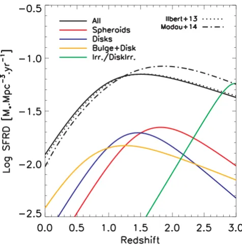
(integrated over all galaxies with log(M_∗/M)≥8). Since this lower limit lies below the completeness limit, the result relies on extrapolating the best Schechter fits to low masses. We first observe the previously reported double-speed growth of the mass density on the full sample (black line) in good agreement with previous measurements. Fromz∼4 to 1, the total mass density increases by a factor of∼6. Fromz∼1 onwards, the growth flattens:ρ_∗atz= 0 is larger by only a factor of∼2. As we discuss in the following sections, this is a consequence of both the decrease in the specific

star formation rate belowz∼1 (e.g. Schreiber et al.2016) and of quenching at large stellar masses.

Regarding the morphological evolution above 108_{solar masses} (resulting from the extrapolation of the best Schechter fits), the key observed trends observed in Fig.5are as follows.

(i) At z > 2, more than 70 per cent of the stellar mass den-sity is in irregular galaxies (see also Conselice et al. 2005). The stellar mass density in irregulars decreases over time from

(10)

[image:10.595.44.547.59.396.2]

Figure 5. Evolution of the stellar mass density for galaxies with log(M_∗/M)>108_{. The left-hand panels show the full sample. The middle and right-hand}

panels show star-forming and quiescent galaxies, respectively. The different colours correspond to different morphologies as labelled. Bottom line are fractions. The pink triangles and brown squares are measurements from Ilbert et al. (2013) and Muzzin et al. (2013).

log(ρ_∗/MMpc−3₎_∼₇_._{7 at}_z_∼_{1.5 to}_∼_{7.1 at}_z_∼_{0.3. This is} clear evidence of morphological transformations as we will discuss in the following sections.

(ii) Atz >2, 30 per cent of the stellar mass density is in compact spheroids with large B/T. This suggests that bulge growth at this epoch destroys discs.

(iii) The emergence ofregular discs(S0a-Sbc) happens between

z∼2 andz∼1. In this period, the stellar density in both pure discs and bulge+disc systems increases by a factor of∼30.

(iv) Belowz∼1, the stellar mass density is equally distributed among discs, spheroids and mixed systems.

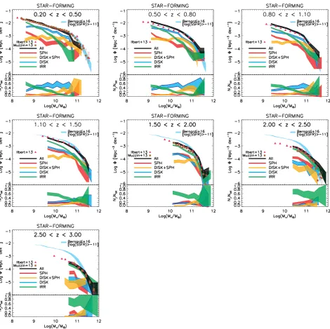
4.2 Evolution of the star-forming population

Fig. 6shows the evolution of the SMFs of star-forming galaxies as a function of morphological type. To guide the eye, the cyan region (same in all panels) shows thez∼0.1 SDSS determination as a reference. This curve was obtained by following the analysis of Bernardi et al. (2016), but selecting the subset of objects for which the log of the specific star formation rate determined by the MPA-JHU (e.g. Kauffmann et al.2003) group is greater than−11 dex.

Table2summarizes the best-fitting Schechter function parame-ters for our CANDELS analysis. In agreement with previous work, the SMF of all star-forming galaxies increases steeply at the low-mass end, and evolves very little at the high-low-mass end. This is

a consequence of quenching: when star-forming galaxies exceed a critical mass, they quench and so are removed from the star-forming sample (e.g. Peng et al.2010; Ilbert et al.2013).

Our new results show that the morphological mix of star-forming galaxies also experiences a pronounced evolution. At 0.2< z < 0.5, the typical morphology of a star-forming galaxy differs sig-nificantly from that in the full sample. Purely bulge-dominated systems (spheroids) account for≤5 per cent of the objects at all stellar masses. Star-forming galaxies at low redshifts are therefore dominated by regular systems with no pronounced asymmetries and with low bulge fractions (i.e. discs) over two decades in stellar mass (9<log(M∗/M)<11). Irregular discs start to dominate only at very low masses (log(M_∗/M)≤9). Bulge+disc systems are also a minority, but account for∼40 per cent of the population at stellar masses greater than log(M_∗/M)∼10.7. The presence of the bulge component is therefore tightly linked to the star for-mation activity of the galaxy as widely documented in the recent literature (e.g. Wuyts et al.2012). As observed for the full sample, this morphological mix seems to have remained rather stable since

z∼1.

At higher redshifts, the relative abundance of irregulars and nor-mal discs is inverted: disturbed systems become the dominant mor-phological class of star-forming galaxies. The relative abundance steadily increases fromz∼1 toz∼2. Atz >2, irregular systems are almost 100 per cent of the star-forming population. While we confirm a population of star-forming spheroids atz >2 (e.g. van