Design and implementation of a loss optimization control for electric vehicle in wheel permanent magnet synchronous motor direct drive system

Design and Implementation of a Loss Optimization Control

for Electric Vehicle In-Wheel Permanent-Magnet

Synchronous Motor Direct Drive System

Qingbo Guo

a

, ChengMing Zhang

a*

, Liyi Li

a

, David Gerada

b

, Jiangpeng Zhang

a

,

Mingyi Wang

a1

a_{Department of Electrical Engineering Harbin Institute of Technology, No. 2 of Yikuang Street, Harbin, 150001. China} b_{PEMC Group, Faculty of Engineering, University of Nottingham, Nottingham, NG72RD. United Kingdom}

Abstract

As a main driving force of electric vehicles (EVs), the losses of in-wheel permanent-magnet synchronous motor (PMSM) direct drive system can seriously affect the energy consumption of EVs. This paper proposes a loss minimization control strategy for in-wheel PMSM direct drive system of EVs which optimizes the losses of both the PMSM and of the inverter. The proposed method adjusts the copper losses and iron losses by identifying the optimal flux-weakening current, which results in the PMSM achieving lower losses in the whole operational range. Moreover as there are strongly nonlinear characteristics for the power devices, this paper creates a nonlinear loss model for three-phase half-bridge inverters to obtain accurate inverter losses under space vector pulse width modulation (SVPWM). Based on the inverter loss model and double Fourier integral analysis theory, the PWM frequency is optimized by the control strategy in order to maximize the inverter efficiency without affecting the operational stability of the drive. The proposed loss minimization control strategy can quickly find the optimum flux-weakening current and PWM frequency, and as a result significantly broaden the high efficiency area of the PMSM direct drive system. The effects of the aforementioned strategy are verified by both theoretical analysis and experimental results.

HIGHLIGHTS

(1) The nonlinear characteristics of the power device are modeled.

(2) The harmonic components of a PWM switched inverter output are solved analytically by double Fourier integral analysis theory.

(3) The proposed control strategy can optimize both the motor losses and inverter losses of a PMSM system. (4) The motor efficiency has been increased by 0.5%, the inverter efficiency has been increased by 6.6%, and the

system efficiency has been increased by 4.6% in a SPMSM system with SiC-MOSFETs. (5) The proposed loss optimization control strategy has been validated by the experimental tests.

Keywords: SiC-MOSFETs; loss optimization control; nonlinear loss model; analytical harmonic model of inverter output; double Fourier integral analysis; PMSM direct drive system.

1

1. Introduction

With the worldwide shortage of energy and increasingly stringent emission requirements, the

improvement of energy efficiency and development of new clean energy have become of increasing

importance to society. With the advantage of high energy efficiency and low emissions, electric

vehicles (EVs) [1,2] and hybrid electric vehicle (HEVs) [3,4] are considered an attractive proposition

to the traditional internal combustion engine vehicles. HEVs are more commonly used for long

distance or heavy load transportation while EVs have a stronger application case for transportation

within cities. As EVs are a battery-powered, limited energy system, the consumption characteristics of

the energy management system are of fundamental importance and an order of magnitude higher in

terms of priority compared to HEVs. As regards the system layout, compared to the traditional motor

drive system with automated mechanical transmission (AMT) [5], the in-wheel motor direct drive

system has the advantages of high dynamic performance and low transmission loss which is more

suitable for EVs, as shown in Fig.1.

(a) (b)

Fig.1.PMSM drive system in EVs; (a) PMSM with AMT; (b) PMSM direct drive system.

To improve the endurance mileage of EVs in one charge, it is important to minimize the energy

consumption. As the main power output mechanism of EVs, any efficiency gains on the traction drive

directly translate to a markedly improved endurance mileage[6].There are several types of electric

motor used within the power system of EVs, such as the direct-current (DC) motor, induction motor

(IM), permanent magnet synchronous motor (PMSM) and switched reluctance motor (SRM). The

PMSM due to its high efficiency, high power factor, and high power density is often the machine of

choice. The operational efficiency of the PMSM drive depends on the motor’s electromagnetic design

and the applied control strategy [7-9]. The electromagnetic design optimization consists of tailoring the

constituent geometries, materials and losses with the aim of improving the efficiency at rated

operation[10-13]. On the other hand control strategies take into consideration the efficiency within the

overall operational range of the drive [14-16]. There are many vector control strategies for PMSM

power system of EVs, such as theid=0 control, unity power factor (UPF) control, maximum torque per

ampere (MTPA) control, maximum speed per voltage (MSPV) control and loss model control (LMC).

Theid=0 control maintains the electromagnetic torque and q-axis current in a proportional relationship

within the linear machine operation mode by keeping the d-axis current to zero [17,18]. The id=0

control is widely used in surface-mounted PMSMs (SPMSMs) due to the lack of saliency. However,

id=0 control cannot maximize the electromagnetic torque in interior PMSMs (IPMSMs), and therefore,

MTPA control is presented to make the most of the inherent saliency and thus available reluctance

torque[19,20]. The MTPA control strategy achieves the minimum copper loss since the least armature

current is used to obtain the desired torque output, however it only optimizes for reducing the copper

losses and will thus not maximize the efficiency of the PMSM which is constituted of various other

loss terms [21-23]. Similarly the MSPV control which minimizes the winding terminal voltage and

decreases the reactive power to zero and thus reduces the energy loss between power transmissions

[24,25], however in doing so it does not focus on the loss of PMSM and can be thus comparatively

inefficient on the machine side[26-30]. The losses of a PMSM can be divided into four parts:

mechanical losses, copper losses, iron losses and stray losses. The copper losses and iron losses are so

-called controllable losses which can be influenced directly by the control strategies. The MTPA

control and MSPV only focus on part of the controllable losses while the LMC takes into consideration

both the copper losses and iron losses and can thus optimize for maximizing the efficiency over the

whole operational range of the PMSM [31,32].

The literature on LMC focuses attention on the motor loss reduction, however the inverter losses also

play an important part in the overall energy consumption characteristics of EVs. Current research on

reducing inverter losses focuses on the modulation mode of the three-phase inverter [33-36], and

ignores the coupling relations between the power converters and the motors which affect the stability of

PMSM system. Other research simply applies SiC power devices to improve the inverter efficiency.

Although SiC power devices with low switching losses decrease the inverter loss and increase the

inverter efficiency of the PMSM system, the resulting low efficiency when the vehicle slows down can

be an issue in EV applications [37-39]. From the foregoing discussion clearly in optimizing the EV

PMSM drive system it is required to take into account the constituent controllable losses of both the

machine and the inverter, while carefully considering the stability and dynamic performance

requirements.

This paper systematically analyzes the losses of a PMSM drive system in EVs and proposes a novel

loss optimization control strategy for PMSM direct drive system which achieves a higher efficiency

compared to traditional vector control over the whole vehicle operational range. Based on the loss

model of the PMSM, the loss optimization control can optimize the copper losses and iron losses

together. In order to characterize the inverter losses accurately, this paper creates a nonlinear loss

model of a three-phase half-bridge inverter in the space vector pulse width modulation (SVPWM). This

research analyses the harmonic component of pulse width modulation (PWM) output voltage in

SVPWM by double Fourier integral analysis, and creates the harmonic model of the PMSM in EVs.

Based on the system loss model, the PWM frequency is carefully adjusted to the direct drive system by

the proposed control method, which decreases the loss of the inverter while ensuring small current

harmonic content. The loss optimization control strategy can reduce the energy consumption without

affecting the stability of the PMSM direct drive system for EVs and is validated both theoretically and

experimentally.

The remainder of this paper is organized as follows. In Section 2, the model for describing the PMSM

direct drive system which considers both the PMSM losses and inverter losses is analysed. In Section

3, based on the model of PMSM direct drive system, the loss minimization control strategy is

developed. In Section 4, the experimental setup is illustrated and the proposed control strategy is

validated by experimental results. Conclusions are then drawn in the final section.

2. Model of PMSM direct drive system

The typical topology of a PMSM drive system is shown in Fig.2. In order to increase the

presents a novel loss model of PMSM considers both the motor and inverter losses. Moreover it

creates a nonlinear loss model of the three-phase half-bridge inverter which analyses the conduction

and switch losses of power devices accurately.

a

U

b

U

c

U

3

V

1

V V₅

4

V V6 V2

PMS M

Fig.2.Typical topology of three-phase PMSM power system.

2.1. Loss model of PMSM

To minimize the PM motor losses , it is important to build a precise loss model . The controllable

loss of PMSM can be divided into two parts, namely the stator copper losses and stator iron losses. The

stator copper loss is caused by the motor current in the armature windings while the stator iron loss is

generated by the flux linkages in the stator and rotor. The mathematical loss models of a PMSM in the

d-axis and q-axis are shown in Fig.3(a) and (b) respecitvely.

(a) (b)

Fig.3.Decoupled mathematics model of PMSM: (a) Dynamic mathematical model in d-axis; (b) Dynamic mathematical model in q-axis.

From Fig.3, the voltage equations of PMSM can be described as :

1

1

0 0

d d d d od

s

q q q q oq

U L di dt i U

R

U L di dt i U

         

  

         

          (1)

0 0 0

0 0

od md od p r mq od

oq m q oq p r md oq p r f

U L di dt n L i

U L di dt n L i n



 



           

  

           

            (2)

whereL1dand L1q are the stator leakage inductances in the d-axis and q-axis, Lmd and Lmq are the

stator self inductances in the d-axis and q-axis respectively,Rsis the stator armature resistance,Rc is

the stator iron loss resistance,npis the pole pair number,ωris the rotational speed, ψfis the magnet

flux linkage,ud,qandid,qare the stator terminal voltage and the armature current respectively,icdandicq

are the iron loss currents , while iod and ioq are the magnetic currents in the d-axis and q-axis

respectively.









od d cd

oq q cq

cd od c md od p r q oq c

cq oq c mq oq p r f d od c

i i i

i i i

i u R L di dt n L i R

i u R L di dt n L i R

       _{ }   _{  }   _{    }    (3)

Based on the voltage and current equations, the stator copper loss can be obtained as :

















2 2 2 2

1.5 ( )

1.5

Cu s d q

od md od p r q oq c

s

oq mq oq p r f d od c

P R i i

i L di dt n L i R

R

i L di dt n L i R

      _{ }     _{ }   _    _    (4)

where the coefficient 1.5 in (4) is a result of the Clark and Park transformations, in which the flux value

remains invariable

The stator iron loss of PMSM can be also described as :









2 2

2

2

1.5 ( )

1.5

1.5

Fe c cd cq

md od p r q oq c

mq oq p r f d od c

P R i i

L di dt n L i R

L di dt n L i R

          _   _ (5)

From equation (4) and equation (5), the fundamental loss can then be derived as :

























_ 2 2 2 2 1.5 1.5 1.5 1.5

loss motor Cu Fe

s od md od p r q oq c

s oq mq oq p r f d od c

md od p r q oq c

mq oq p r f d od c

P P P

R i L di dt n L i R

R i L di dt n L i R

L di dt n L i R

L di dt n L i R

              _    _      _   _ (6)

The major energy loss occurs at steady state conditions, hence (6) can be simplified as :





















_ _ _ 2 2 2 2 1.5 1.5 1.5

loss motor Cu f Fe f

s od p r q oq c oq p r f d od c

p r q oq c p r f d od c

P P P

R i n L i R i n L i R

n L i R n L i R

            _   _     _  _ (7)

From equation (7) the motor loss is only a function of the rotational speed, d-axis current and q-axis

current.

2.2. Loss model of three-phase half-bridge inverter

This section proposes a novel model of the power device which considers the nonlinear characteristics

of both the switching and conduction losses and uses these to analytically predict the nonlinear losses

2.2.1 Inverter Conduction Losses

As shown in Fig.4, there is a high degree of nonlinearity in both the switching and conduction

characteristics of power devices such as MOSFETs and IGBTs. The classical linear model of

conduction characteristics is expressed as :

0

cesat t ds ce

u U R i (8)

whereucesatis the saturation voltage of the power device,Ut0is the equivalent conduction voltage at

rated currentIn,iceis the current through power device, andRceis the equivalent conduction resistance

at the rated currentIn. The main drawback of the aforesaid linear model is that it can only calculate

losses accurately close to the rated current. As the stator current in the PMSM EV drive changes

continuously in a sinusoidal manner a more representative model is required.

U

t0

R

ce

u

ce

I

n

i

ce _Linear

model Nonlinear

model Condcution characteristics

Fig.4.Conduction characteristics of the power devices

From Fig.4. the nonlinear model for the power device conduction characteristics is more

representatively described for the whole operational range by a second order polynomial of the form :

2

cesat c c ce c ce

u  a b i c i (9)

whereac,bcandccare fitting coefficients.

The average conduction losses of the power device in a current period can then be expressed as :

_ ₀

current T

loss conduction ce ce ce current

P 



d u i dt T (10)

whereTcurrentis the current period, anddceis the duty ratio of PWM signal.

2.2.2 Inverter Switching Losses

As with the conduction effects, the switching losses are also highly nonlinear. These can be divided

into two constituent parts namely (i)switch-on loss and (ii)switch-off loss. The nonlinear models for the

switching loss characteristics of the power device can also be described by second order polynomials :



2



_

2 /

on dc on on ce on ce dc test

E  U  a b  i c i U (11)



2



_

2 /

off dc off off ce off ce dc test

E  U  a b  i c i U (12)

where 2Udc is the DC voltage, Udc_test is the DC voltage when the chip manual tested switching

As the switching losses are a function of current, for the sinusoidal EV drive under consideration the

losses in a current period can be expressed as :





_

0 current T

loss switch on off current

P 



E E dt T (13)

2.2.3 Loss model under SVPWM

Based on the described conduction and switching loss models of the power device, the loss model of a

three-phase inverter can be obtained for different modulation modes. As shown in Fig.5, there are only

eight possible switch combinations for a three-phase inverter.

60(110)

U

1 1

( , )

6 2

0(100)

U





120(010)

U

000(000)

U

240(001)

U

300(101)

U

2 ( , 0 )

3

1 1

( , )

6 2



2 ( , 0 )

3



180(011)

U

111(111)

U

1 1

( , )

6 2

  1 1

( , )

6  2

I

II

I

III

IV

V

VI

6

U

1

U

4

U

2

U

3

U

5

U

0

U

7

U

Fig.5.Eight switch states for three-phase inverter.

The state of a phase leg is defined as “1” when the phase leg is open, and as “0” when closed. The U0

(000) state and U7 (111) state correspond to a short circuit on the output, while the other six states can

be considered to form stationary vectors in the d-q complex plane. Each stationary vector corresponds

to a particular fundamental angular position. The SVPWM applies these eight stationary vectors to

form an arbitrary target output vector U0at any point in time by the summation of a number of these

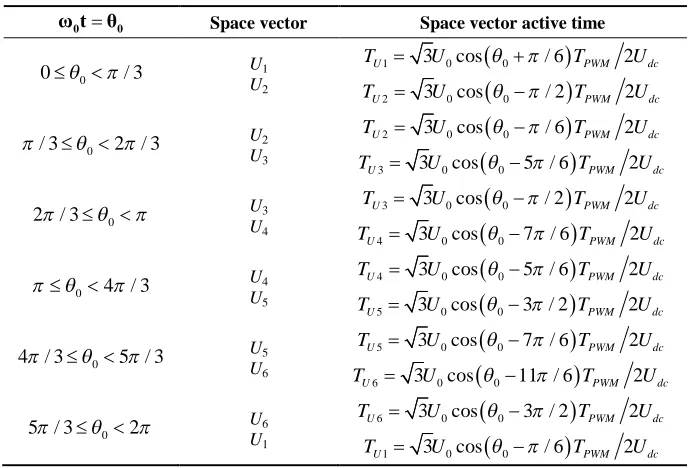
space vectors within one switching period (TPWM). The space vectors and active times for different

target output vectors is shown in Table 1.

Based on Table 1, the duty ratio of a PWM signal on the power device can be calculated by the space

vector active time in SVPWM., hence the conduction loss of an IGBT in the three-phase half-bridge

inverter can be expressed as :







 



 

2

_ ₀

2 ₂

0 0 0

0

2 2

0 0 0 0 0

0

sin sin sin

9

24 16 6 6 cos 3 4 cos 2

8

current

current T

loss conduction ce c c ce c ce ce current T

ce c c current c current current current

c c c c c c

P d a b i c i i dt T

d a b I t c I t I t dt T

a c I b I b I m c I m b I m

I

  

 

    

 

 _     _  

    







 

2

0 0

48

4 3 a m_c cos 16 3b I m_c cos 3 3 c I m_c cos

 

    

 

 

 

  

 

 

where I0 is the amplitude of the motor’s sinusoidal phase current, ωcurrent is the current’s angular

frequency,φis the power factor angle andmis the modulation ratio for SVPWM, defined as :

0

3 2 _dc

m U U (15)

[image:8.595.125.471.194.428.2]

whereU0is the line-to-line voltage amplitude.

Table 1.Space vector and active time in the SVPWM.



0 0

ω t θ Space vector Space vector active time

0

0 / 3 U1

U2





1 3 0cos 0 / 6 2

U PWM dc

T  U   T U





2 3 0cos 0 / 2 2

U PWM dc

T  U   T U

0

/ 3 2 / 3

    U2

U3





2 3 0cos 0 / 6 2

U PWM dc

T  U   T U





3 3 0cos 0 5 / 6 2

U PWM dc

T  U    T U

0

2 / 3   U3

U4





3 3 0cos 0 / 2 2

U PWM dc

T  U   T U





4 3 0cos 0 7 / 6 2

U PWM dc

T  U    T U

0 4 / 3

    U4

U5





4 3 0cos 0 5 / 6 2

U PWM dc

T  U    T U





5 3 0cos 0 3 / 2 2

U PWM dc

T  U    T U

0

4 / 3  5 / 3 U5

U6





5 3 0cos 0 7 / 6 2

U PWM dc

T  U    T U





6 3 0cos 0 11 / 6 2

U PWM dc

T  U    T U

0

5 / 3  2 U6

U1





6 3 0cos 0 3 / 2 2

U PWM dc

T  U    T U





1 3 0cos 0 / 6 2

U PWM dc

T  U   T U

The conduction loss of the freewheeling diode (FWD), switching loss of IGBT, and recovery loss of

FWD can be calculated in the similar way to conduction loss of IGBT. Therefore, the nonlinear loss

model of the power converter under SVPWM can be expressed as :







 















 

_

_

 

















_ 2

0 0 0

2 0 0 0 0 2 0 2 0 6

24 16 6 6

9 8 cos 3 4 cos 2

48

4 3 cos 16 3 cos

6

3 3 cos

2 4

loss power IGBT FWD

c f c f c f c f

c f c f

c f c f

c f

sw dc on off rec on off

P P P

a a c c I b b I b b I m

c c I m b b I m

I

a a m b b I m

c c I m

f U c c c I b b

                                          

    



 brec



I0 



aon aoff arec



2 Udc test_

                        _{ }    (16)

wherePFWD is the loss of freewheeling diode. af,bfandcfare the fitting coefficients for conduction

characteristics of FWD. arec, brec, and crec are the fitting coefficients for recovery characteristics of

FWD. andfswis the PWM frequency.

3. Loss optimization control strategy

From the previous sections discussing the loss models of the motor and PE converter, it can be seen

that the loss of the direct drive system in consideration is a fairly complex function, as described by





















 





 

















_ _ _ 2

0 0 0

2 0 0 0 0 2 0 0

24 16 6 6

9 8 cos 3 4 cos 2

48

4 3 cos 16 3 cos

6

3 3 cos

2

loss system loss motor loss power

c f c f c f c f

c f c f

c f c f

c f sw dc on off rec

P P P

a a c c I b b I b b I m

c c I m b b I m

I

a a m b b I m

c c I m

f U c c c I

                                             





























2 0 _ 2 2 2 2 4 2 1.5 1.5 1.5

on off rec on off rec dc test s od p r q oq c oq p r f d od c

p r q oq c p r f d od c

b b b I a a a U

R i n L i R i n L i R

n L i R n L i R

                                  _{ }        _   _     _  _ (17)

whereI0can be obtained as :













2 2 0 2 2 d q

md od p r q oq c od

mq oq p r f d od c oq I i i

L di dt n L i R i

L di dt n L i R i

               _   _  (18)

The power factorcan be calculated from :





 

arctan u ud q arctan i id q

   (19)

Due to the complexity of the loss model it is impossible to obtain the optimal working point by means

of direct analysis. In light of the aforesaid this paper proposes a quick and simple loss minimization

control strategy which divides the system losses into two parts, namely (i)the losses affected by PMSM

operation condition and (ii) the losses affected by the inverter state :

_ _ _

loss system loss PMSM loss inverter

P



P



P

(20)

The loss affected by the PMSM operation condition can be written as :





















 





 

























2

0 0 0

2 0 0 _ 0 0 2 0 2 2

24 16 6 6

9 8 cos 3 4 cos 2

8

4 3 cos 16 3 cos

3 3 cos

1.5 1.5

c f c f c f c f

c f c f

loss PMSM

c f c f

c f

s od p r q oq c oq p r f d od c

a a c c I b b I b b I m

c c I m b b I m

P I

a a m b b I m

c c I m

R i n L i R i n L i R

n                                                _   _







2





2

1.5

prL iq oq Rc np r f L id od  Rc

(21)

while the loss affected by the inverter state can be expressed as :





2









_ 12 0 4 0 2 _

loss inverter sw dc on off rec on off rec on off rec dc test

P  f U _ c c c I  b b b I  a a a _ U (22)

The proposed control method can improve the system efficiency by optimizing these two parts of

system loss in an analytical manner. In addition, the coupling relation between motor and inverter is

also considered by the loss minimization control strategy.

From equation (21) Ploss_PMSM consists of inverter conduction losses together with the PMSM losses.

Compared with motor loss, the inverter conduction loss is much smaller in magnitude and hence can be

ignored for efficiency optimization purposes. Equation (21) also shows that the controllable part of loss

affected by PMSM state is a function of d-axis magnetic current iod, angular speed ωr and q-axis

magnetic currentioq:





_ , ,

loss PMSM od r oq

P  f i  i (23)

The electromagnetic torque equation of PMSM can be described as





1.5

e p f oq md mq od oq

T  n _ i  L L i i _ (24)

From equation (24), the q-axis magnetic currentioqcan be expressed as a function of electromagnetic

torqueTeand the d-axis magnetic currentiod.





1.5

oq e p f md mq od

i T n _  L L i _ (25)

Substituting equation (25) into equation (23), the controllable part of loss affected by PMSM operation

condition can befurther simplified as :













_ , , 1.5 , ,

loss PMSM od r e p f md mq od od r e

P  f i  T n _  L L i _  f i  T (26)

Equation (26) shows that the controllable part of loss affected by PMSM operation condition can be

expressed as a function of the rotational speed ωr, the d-axis magnetic current iod and the

electromagnetic torqueTe. Therefore for a given toque demand at a given speed, there exists an optimal

flux-weakening d-axis magnetic current which can yield the maximum efficiency. The optimal d-axis

magnetic currentiod*can be obtained from equation (26) as :





*

,

_ 0

r e

od od const T const loss PMSM od

i i

P i   



   (27)

From equation (27) the loss optimization control strategy can optimize the stator copper loss and stator

iron loss together, and decrease the motor loss in the whole operation range of EVs. However, the

optimal currentiod

*

is limited by two aspects. The first aspect is that the optimal current in the d-axis

must be less than the maximum flux-wakening current which will cause irreversible magnet

demagnetization :

*

_ _

od d permenent magnet

i i (28)

whereid_permanet_magnentis the maximum flux-wakening current of permanent magnet in the PMSM.

The second aspect is that the optimal d-axis current is limited by the maximum inverter current :

2 2 2

_ max

d q s

i  i I (29)

whereIs_maxis the maximum current of inverter.

For the case of surface-mount PM machines (SPMSMs), the non-salient rotor structure makes the stator

self-inductance in the d-axis equal to that in the q-axis. Therefore, the optimal operation point of the









2 2 2 2 2 2

od p r s f s c p r s s c s c

i  n  L R R n  L R R R R (30)

whereLsis the stator inductance of SPMSM,

s md mq

L L L (31)

3.2. Optimization on the loss affected by inverter state

From the previously discussed equation (27) it was shown that there is an optimal current which

minimizes both the copper and iron losses. By applying the aforesaid optimal current to the PMSM

drive system, the loss affected by the inverter state is then only a function of the PWM frequency :













2 0

_ 0 _

0

4

12

2

( , , )

on off rec

loss inverter sw dc on off rec dc test

on off rec sw dc

c c c I

P f U b b b I U

a a a

f f U I



   

 

 

    

 

   

 



(32)

Hence the inverter losses can be decreased by reducing the switching frequency of the PWM signal.

However as the motor is fed by a PWM inverter there are several harmonic currents in the stator

windings, the magnitude of which will increase with lowering the switching frequency. For the

application in hand, being a direct-drive system, the motors are directly connected to the load, therefore

the large harmonic stator current affects the overall drive stability. It is thus critical to obtain the

harmonic content with different PWM switching frequencies.

Determination of the harmonic frequency components of a PWM switched inverter output is quite

complex and is often done by using a fast Fourier transform (FFT) analysis of a simulated time-varying

switched waveform. This approach reduces the mathematical effort, but it still requires considerable

computing capacity and leaves uncertainty as to whether a subtle simulation round-off or error may

have affected the results obtained. In contrast, an analytical solution using double Fourier integral

analysis can exactly identify the harmonic components of a PWM waveform, and is thus used within

the loss optimization control strategy In double Fourier integral analysis theory, the PWM output

voltage of the inverter can be obtained by two time variables, x(t) and y(t), where x(t) is the carrier

signal and y(t) is the fundamental (sinusoid) signal.

( ) c c

x t t (33)

where ωc is the carrier angular frequency and θc is the arbitrary phase offset angle for the carrier

waveform.

0 0

( )

y t t (34)

where ω0 is the fundamental angular frequency and θ0 is the arbitrary phase offset angle for the

fundamental waveform.

The output voltage of the inverter leg can be described as :

2 ( ) ( )

( ) ( ( ), ( ))

0 ( ) ( )

d c n

U y t x t a t f x t y t

y t x t

 

 _{ }



where 2Udcis the DC voltage as shown in Fig.2. The output voltage of the inverter leg is defined with

respect to the negative DC bus rather than to the midpoint of the DC bus, in order to simplify the

mathematics of the Fourier solution.

With double Fourier integral analysis theory [40,41], the time-varying function f(x(t),y(t)) can be

expressed as a summation of the harmonic components :



























 





 



00 0 0 0 0 0 0

1

0 0

1

0 0

1 _{0 0}

( 0)

( , ) 2 cos sin

cos sin

cos sin

n n

n

m c c m c c

m

mn c c

m n _{mn c c}

n

f x y A A n t B n t

A m t B m t

A m t n t

B m t n t



 



 

  

  _    _ _    _

 _    _ _    _

          

   

  

         

  

 





 

(36)

whereA00is the DC offset;A0nandB0nare the fundamental component and base-band harmonics;Am0

andBm0are the carrier harmonics;AmnandBmnare side-band harmonics.

Based on the double Fourier integral analysis, the fundamental component and harmonics of the inverter leg output can then be calculated as





(1 cos )

2 2

(1 cos ) 2

2 exp ( ) 2

M y

mn mn dc

M y

A jB U j mx ny dxdy



 

   

 

_{ }

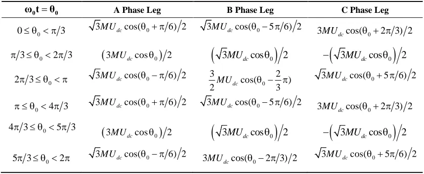
  (37)

[image:12.595.190.425.170.254.2] [image:12.595.83.512.401.577.2]

From Table 1, the phase leg reference voltage for SVPWM can be obtained as described in Table 2.

Table 2.Phase reference voltage for SVPWM. 

0 0

ω t θ A Phase Leg B Phase Leg C Phase Leg

0

0    3 3MUdccos(  0 6) 2 3MUdccos(  0 5 6) 2

0

3MU_dccos(  2 3) 2

0

3 2 3

    



3MU_dccos₀



2



3MU_dccos₀



2 



3MU_dccos₀



2

0

2    3 3MUdccos(  0 6) 2

0

3 2

cos( )

2MUdc   3

0

3MU_dccos(  5 6) 2

0 4 3

     3MUdccos(  0 6) 2 3MUdccos(  0 5 6) 2

0

3MU_dccos(  2 3) 2

0

4    3 5 3

_

_

0

3MU_dccos 2



3MU_dccos₀



2 



3MU_dccos₀



2

0

5    3 2 3MUdccos(  0 6) 2

0

3MU_dccos(  2 3) 2 3MUdccos(  0 5 6) 2

Table 2 shows that the phase reference signal for SVPWM is not a continuous function, but is made up

of six segments, each spanning 60° for a complete fundamental cycle :





2 2

1 1

6 _{( ) ( )}

2 ( ) ( )

1

2 exp ( ) 2

y i x i mn mn _{y i x i} dc

i

A jB U j mx ny dxdy



 

 

  (38)

The outer and inner integral limits of equation (38) are defined in Table 3. From equation (35), the

































00 0 0 0 0

1 0 0 1 0 0 1 ( 0)

( ) 2 cos sin

cos sin

cos sin

az n n

n

m c c m c c

m

mn c c mn c c

m n n

u t A A n t B n t

A m t B m t

A m t n t B m t n t

[image:13.595.99.506.350.512.2]

           _    _  _    _ _    _  _      _ _      _





 

(39)

Table 3.Outer and inner integral limits for SVPWM.

i y1(i) y2(i) x1(i) x2(i)

1 2 / 3    [1 3Mcos(y / 6) 2] 2  [1 3Mcos(y / 6) 2] 2

2 / 3 2 / 3  (1 3Mcosy 2) 2  (1 3Mcosy 2) 2

3 0 / 3   [1 3Mcos(y / 6) 2] 2  [1 3Mcos(y / 6) 2] 2

4 / 3 0   [1 3Mcos(y / 6) 2] 2  [1 3Mcos(y / 6) 2] 2

5  2 / 3 / 3   (1 3Mcosy 2) 2  (1 3Mcosy 2) 2

6   2 / 3   [1 3Mcos(y / 6) 2] 2  [1 3Mcos(y / 6) 2] 2

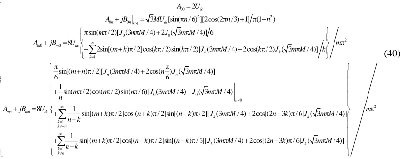
The harmonic coefficients can be expressed as :

00

2 2

0 0 1

0 0

2

0 0

1

2

3 [sin( / 6) ][2cos(2 / 3) 1] (1 ) sin( / 2)[ (3 / 4) 2 ( 3 / 4)] 6

8

2sin[( ) / 2]cos( / 2)sin( / 2)[ (3 / 4) 2cos( / 2) ( 3 / 4)]

dc

n nn dc

m m dc

k k

k

mn mn

A U

A jB MU n n n

m J m M J m M

A jB U m

m k k k J m M k J m M k

A jB                                      



0 0 0 1

sin[( ) / 2][ (3 / 4) 2cos( ) ( 3 / 4)]

6 6

1

sin( / 2)cos( / 2)sin( / 6)[ (3 / 4) ( 3 / 4)]

8 1

sin[( ) / 2]cos[( ) / 2]sin[( ) / 2][ (3 / 4) 2cos[(2 3 ) / 6] ( 3 / 4)]

n n n dc k k k k n

m n J m M n J m M

m n n J m M J m M

n U

m k n k n k J m M n k J m M

n k      _{   }  _         _{           } 



2 1 1

sin[( ) / 2]cos[( ) / 2]sin[( ) / 6][ (3k / 4) 2cos[(2 3 ) / 6] ( 3k / 4)]

k k n

m

m k n k n k J m M n k J m M

n k             _{ }  _{ }                            _{           }         



(40)

where the constant termA00is caused by the output voltage definition with respect to the negative DC

bus as previously discussed. The harmonic voltage in equation (39) is also calculated with respect to

the negative DC bus, hence the harmonic voltage with respect to the neutral point can be obtained as





3

nm nm nm nm nm

an az az bz cz

u





u





u





u





u



(41)

where

nm az

u ,

nm bz

u and

nm bz

u are the harmonic voltages with respect to the negative DC bus in then-th

fundamental signal and them-th carrier signal. In addition,

nm an

u is the harmonic voltage with respect

to the load neutral point in thenth fundamental signal and them-th carrier signal.

Based on equation (41), the stator harmonic current can be obtained as





nm nm

s an s mn s

I u R  j L (42)

From equation (42), the loss minimization control can acquire the optimal PWM frequencyfPWM*by the

01

*

max

1 2

0 ( 0)

mn mn

PWM PWM

A A A

m n n

n m

f f

i i i THD

  

  

  _

 

 _  _

 

 

 

 



(43)

whereTHDmaxis the maximum motor current THDpermissible for each EV operational condition in

order to keep the system stable.

Hence by adjusting the flux-weakening currentiodto the optimumiod*and the PWM frequencyfPWMto

the optimal frequencyfPWM

*

, the proposed PMSM control strategy can achieve lower overall losses in

the whole EV operation range compared to traditional control strategies, while ensuring drive stability.

The structure diagram of the loss minimization control system is shown in Fig.6.

a

i

c

i

PWM



dq

* d

i * q

i

* d u

* q u

*

α

u *

β

u

d i

q i

e

 sα

i

sβ

i

+ +

-PI u*abc

abc 

PMSM

b i

PI Loss

Optimization Controller

d dt

Throttle

Resolver *

PWM f

e

 ref

T

Dynamometer for EV/HEV Speed

Torque

Fig.6.Proposed PMSM direct drive system. 4. Experiment Study

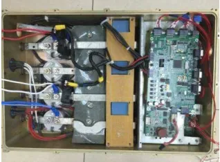
In order to verify the effectiveness of the proposed control strategy with respect to conventional control,

an experimental platform is designed and implemented as shown in Fig.7. A flowchart describing the

steps within the experimental method is shown in Fig.8.

A U

B U

C U

3

V

1

V V₅

4

V V6 V2

(c)

Fig.7.Experimental platform of PMSM system. (a) SiC- MOSFETs based converter; (b) Physical prototype experimental platform; (c) The structure schematic diagram of the experimental platform.

Motor current and speed sample

Based on equation (27), calculate optimal d-axis currentid*

*

_ _

od d permenent magnet i i

Calculate modulation ratio of

PMSM system

Find the optimal PWM frequency by

look-up table method

Find the current control coefficients

by look-up table method

Control the motor current to the command value *2 *2 2

_ max

d q s i i I

*

_ _

od d permenent magnet i i

* * 2 *2 *2

_ max

* * 2 *2 *2

_ max

d d s d q

q q s d q

i i I i i

i i I i i

   

 

  



No

Yes

Yes No

Fig.8.Flowchart of the proposed method in the experimental PMSM.

The proposed control strategy calculates the optimal d-axis currentid

*

by equation (27), and limits the

optimal d-axis currentid*by equation (28) and (29). The optimal PWM frequency is then calculated

off-line by equation (43). The control method applies the optimal PWM frequency and current control

coefficients by means of a hysteresis look-up table. In order to maintain the stability of the

experimental system, the command d-axis current is gradually reduced to the optimal d-axis current.

The three-phase half-bridge inverter utilized is based on the SiC-MOSFET modules (CAS300M12BM2)

which can obtain lower switching losses compared to Si-IGBTs. The inverter is controlled by the

minimization control strategy on the PMSM direct drive system. The motor used within the

[image:16.595.91.505.133.276.2]

experimental setup is a 30kW outer rotor surface PMSM, the parameters of which are listed in Table 4.

Table 4.Model parameters of PMSM.

Parameter Value

Rate power 30kW

Rate speed 360rpm

Poles 22

Slots 24

Phase resistance 0.06Ω

Phase inductance 3.18mH

Flux linkage 0.623Wb

DC link range 360-420V

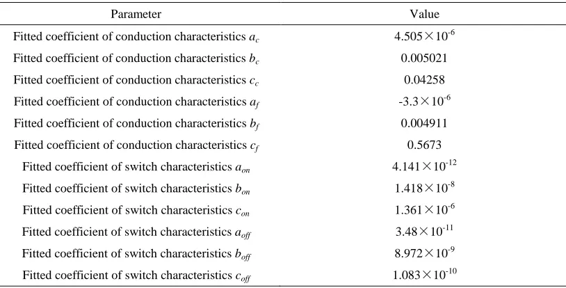
Based on experimentation, the module switch-on voltage is chosen as 15V, while the switch-off

voltage is designed as -5V. The fitting coefficients of CAS 300M12BM2 are listed in Table 5.

Table 5.Fitting coefficients of SiC-MOSFET modules.

Parameter Value

Fitted coefficient of conduction characteristicsac 4.505×10

-6

Fitted coefficient of conduction characteristicsbc 0.005021 Fitted coefficient of conduction characteristicscc 0.04258 Fitted coefficient of conduction characteristicsaf -3.3×10-6 Fitted coefficient of conduction characteristicsbf 0.004911 Fitted coefficient of conduction characteristicscf 0.5673

Fitted coefficient of switch characteristicsaon 4.141×10-12 Fitted coefficient of switch characteristicsbon 1.418×10-8 Fitted coefficient of switch characteristicscon 1.361×10-6 Fitted coefficient of switch characteristicsaoff 3.48×10-11 Fitted coefficient of switch characteristicsboff 8.972×10

-9

Fitted coefficient of switch characteristicscoff 1.083×10-10

A 120kW, 3000rpm eddy current dynamometer serves as the mechanical load. The speed-increasing

gear box is used to increase the maximum rotational speed of the PMSM to the rated speed of the eddy

current dynamometer. As a surface PM machine is used within the experimental setup, the inductance

in the d-axis is equal to that in the q-axis, hence the MTPA control strategy usesid=0. The experimental

results of the selected PMSM direct drive system under MTPA control are shown in Table 6 and Table

7. Table 6 shows the experimental results of SiC-MOSFET based PMSM drive system corresponding

to different powers at rated speed, while Table 7 shows the experimental results corresponding to

[image:16.595.96.503.368.575.2]

[image:17.595.86.501.89.265.2]

Table 6.Experimental results at rated speed under MTPA control.

Output torque (N·m)

Motor current (A)

Mechanical power (kW)

Motor input power

(kW)

System input power

(kW)

Motor efficiency

Inverter efficiency

System efficiency

725 93.1 27.33 29.66 30.13 92.05% 98.55% 90.72%

600 76.3 22.62 24.57 24.81 92.08% 99.02% 91.17%

500 63.1 18.85 20.52 20.79 91.87% 98.69% 90.67%

400 50.5 15.08 16.52 16.85 91.28% 98.02% 89.47%

300 38.3 11.31 12.57 12.91 89.95% 97.37% 87.58%

200 26.3 7.54 8.68 9.11 86.89% 95.25% 82.76%

[image:17.595.85.501.319.493.2]

100 14.7 3.77 4.84 5.37 77.90% 90.09% 70.18%

Table 7.Experimental results at rated torque under MTPA control.

Speed of PMSM

(rpm)

Motor current (A)

Mechanical power (kW)

Motor input power

(kW)

System input power

(kW)

Motor efficiency

Inverter efficiency

System efficiency

360 93.1 27.33 29.66 30.13 92.05% 98.55% 90.72%

300 92.9 22.77 24.77 25.77 91.92% 98.43% 90.47%

250 92.7 18.98 20.73 21.34 91.55% 97.13% 88.92%

200 92.3 15.18 16.73 17.67 90.76% 94.69% 85.94%

150 91.9 11.39 12.78 13.86 89.15% 92.16% 82.16%

100 91.4 7.59 8.86 10.12 85.65% 87.60% 75.02%

50 90.8 3.80 5.00 6.47 75.93% 77.30% 58.69%

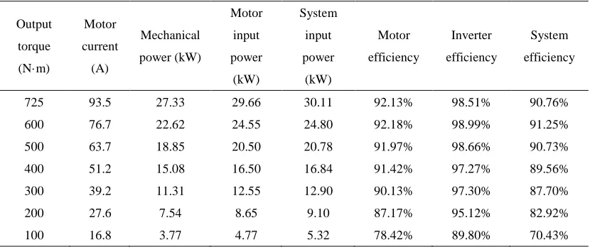
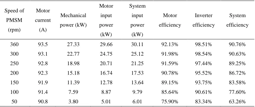
The loss optimization control strategy carefully optimizes the stator current and PWM frequency at

each working point and can achieve higher system efficiency across the whole operation range. Table 8

and Table 9 show the experimental results for the loss optimization control strategy.

Table 8.Experimental results at rated speed for the proposed loss optimization control.

Output torque (N·m)

Motor current (A)

Mechanical power (kW)

Motor input power

(kW)

System input power

(kW)

Motor efficiency

Inverter efficiency

System efficiency

725 93.5 27.33 29.66 30.11 92.13% 98.51% 90.76%

600 76.7 22.62 24.55 24.80 92.18% 98.99% 91.25%

500 63.7 18.85 20.50 20.78 91.97% 98.66% 90.73%

400 51.2 15.08 16.50 16.84 91.42% 97.27% 89.56%

300 39.2 11.31 12.55 12.90 90.13% 97.30% 87.70%

200 27.6 7.54 8.65 9.10 87.17% 95.12% 82.92%

[image:17.595.86.501.586.760.2]

[image:18.595.87.501.90.265.2]

Table 9.Experimental results at rated torque for the proposed loss optimization control.

Speed of PMSM

(rpm)

Motor current (A)

Mechanical power (kW)

Motor input power

(kW)

System input power

(kW)

Motor efficiency

Inverter efficiency

System efficiency

360 93.5 27.33 29.66 30.11 92.13% 98.51% 90.76%

300 93.1 22.77 24.75 25.12 91.98% 98.54% 90.63%

250 92.8 18.98 20.71 21.25 91.59% 97.44% 89.25%

200 92.3 15.18 16.74 17.53 90.78% 95.52% 86.72%

150 91.9 11.39 12.78 13.64 89.15% 93.75% 83.58%

100 91.4 7.59 8.87 9.79 85.64% 90.61% 77.60%

50 90.8 3.80 5.01 6.01 75.90% 83.34% 63.26%

The experimental results from Table 6 to Table 9 verify that the proposed control strategy can increase

the system efficiency for all considered cases. Fig.9. compares the motor current for both the

implemented control strategies, showing that the difference increases as the motor torque is reduced.

[image:18.595.106.485.338.494.2]

(a) (b)

Fig.9 Motor current with two control strategies in the rated speed. (a) Motor current; (b) Difference of motor current.

[image:18.595.105.485.553.712.2]

(a) (b)

Fig.10 Motor efficiency with two control strategies in the rated speed. (a) Motor efficiency; (b) Difference of motor efficiency.

100 200 300 400 500 600 700 800 10

20 30 40 50 60 70 80 90 100

Torque/(N·m)

M

o

to

r

c

u

rr

e

n

t/

A

MTPA control Loss optimization control

100 200 300 400 500 600 700 800 0.5

1 1.5 2

Torque/(N·m)

M

o

to

r

c

u

rr

e

n

t/

A

100 200 300 400 500 600 700 800 0.76

0.78 0.8 0.82 0.84 0.86 0.88 0.9 0.92 0.94

Torque/(N·m)

M

o

to

r

e

ff

ic

ie

n

cy

MTPA control Loss optimization control

100 200 300 400 500 600 700 800 0.5

1 1.5 2 2.5 3 3.5 4 4.5 5 5.5x 10

-3

Torque/(N·m)

E

ff

ic

ie

n

c

y

As shown in Fig.10 which compares the motor efficiency at rated speed (360rpm) under different

control, the proposed control strategy yields a better motor efficiency improvement entitlement

especially when the difference between the iron losses and copper losses is higher (i.e. when the torque

is lower), with the maximum improvement of 0.52% achieved at rated speed for the case of 100Nm.

By the combined optimization of the motor and the SiC-MOSFET converter, the loss optimization

control strategy can enhance the system efficiency by up to 0.25% at rated speed as shown in Fig.11.

(a) (b)

Fig.11 System efficiency with two control strategies in the rated speed. (a) System efficiency; (b) Difference of system efficiency.

(a) (b)

Fig.12 (a)Difference of motor current between MTPA control and proposed control in the rated torque (b) Proportion of optimal d-axis current with motor current in the proposed control method

Fig.12 (a) compares the motor current corresponding to the different control methods for different

speeds. It is noted that the developed control uses a higher current at high speeds (i.e. higher copper

losses), but this is because of an increasing amount of d-axis current, as shown in Fig.12(b) which has

the effect of opposing the magnet flux thereby reducing the iron losses, and minimizing the overall

machine losses

The difference of inverter efficiency with the two control strategies at the rated torque (720 Nm) is

hsown in Fig.13.

100 200 300 400 500 600 700 800 0.7

0.75 0.8 0.85 0.9 0.95

Torque/(N·m)

M

o

to

r

e

ff

ic

ie

n

cy

MTPA control Loss optimization control

100 200 300 400 500 600 700 800 0

0.5 1 1.5 2 2.5x 10

-3

Toeque/(N·m)

E

ff

ic

ie

n

c

y

Difference of two control strategies

50 100 150 200 250 300 350 400 90.5

91 91.5 92 92.5 93 93.5

Speed/rpm

M

o

to

r

c

u

rr

e

n

t/

A

MTPA control optimizatioin control

50 100 150 200 250 300 350 400 0

1 2 3 4 5 6 7 8 9

Speed/rpm

P

ro

p

o

rt

io

n

o

f

o

p

ti

m

a

l

d

-a

x

is

cu

rr

e

n

t/

(a) (b)

Fig.13. Inverter efficiency with two control strategies at rated torque. (a) Inverter efficiency; (b) Difference of inverter efficiency.

The loss optimization control can decrease the inverter losses almost the entire speed range of EVs. By

using SiC-MOSFETs as the power devices, the switching losses of the inverter are reduced and an

inverter efficiency of 98.51% efficiency is obtained at the high speed end. It is noted that the efficiency

of the inverter is reduced when the motor slows down. However by optimizing the stator current and

PWM switching frequency, the proposed loss minimization control strategy can improve the inverter

efficiency by about 6% at low speeds. Of note, fig.13 also shows that the inverter efficiency at 350rpm

is lower by the proposed loss optimization control. This is caused by the increased stator current in the

d-axis. The control strategy is based on the operation condition of PMSM drive system and at the

aforementioned point although the converter efficiency will be slightly worse, this is outweighed by the

gains in the overall system efficiency which is shown in Fig.14.

(a) (b)

Fig.14. System efficiency with two control strategies in the rated torque. (a) System efficiency; (b) Difference of system efficiency.

From Fig.14 compared with traditional MTPA control, the loss minimiztion control strategy can reduce

the system loss at each working point of EVs. Although the system efficiency of PMSM direct drive

system reaches 90.76% at the rated operation point by traditional MTPA control, the loss optimization

control method improves the system efficiency by 4.6% at low speeds, and thus broadens the high

efficiency drive operation area which is very important to EVs.

50 100 150 200 250 300 350 400 0.75

0.8 0.85 0.9 0.95 1

Speed/rpm

In

v

e

rt

e

r

e

ff

ic

ie

n

c

y MTPA control

Loss optimization control

50 100 150 200 250 300 350 400 -0.01

0 0.01 0.02 0.03 0.04 0.05 0.06 0.07

Speed/rpm

E

ff

ic

ie

n

c

y

Difference of two control strategies

50 100 150 200 250 300 350 400 0.55

0.6 0.65 0.7 0.75 0.8 0.85 0.9 0.95

Speed/rpm

E

ff

ic

ie

n

c

y MTPA control

loss optimization control

50 100 150 200 250 300 350 400 0

0.005 0.01 0.015 0.02 0.025 0.03 0.035 0.04 0.045 0.05

Speed/rpm

E

ff

ci

e

n

c

y

As the switching losses in Si-IGBTs are higher than the switching losses in SiC-MOSFETs, it follows

that the proposed optimization control method should yield higher efficiency improvement when

implemented on a traditional Si-IGBT-based converter. To this end the same motor is tested using a

Si-IGBT (FF300R06KE3_BE2) based power converter shown in Fig.15, with the experimental results

at rated torque under MTPA and under the developed control method listed in Table 10 and Table 11

[image:21.595.228.387.185.302.2]

respectively.

[image:21.595.111.485.367.542.2]

Fig.15 Si-IGBT based power converter for PMSM direct drive system.

Table 10.Experimental results of Si-IGBT based PMSM system at rated torque in the MTPA control.

Speed of PMSM

(rpm)

Mechanical power (kW)

Motor input power

(kW)

System input power

(kW)

Motor efficiency

Inverter efficiency

System efficiency

360 27.33 29.9 30.93 92.05% 95.98% 88.34%

300 22.77 24.77 26.04 91.92% 95.11% 87.42%

250 18.98 20.73 22.39 91.55% 92.57% 84.74%

200 15.18 16.73 18.38 90.76% 91.02% 82.60%

150 11.39 12.78 14.62 89.15% 87.43% 77.94%

100 7.59 8.86 10.76 86.65% 82.36% 70.54%

50 3.80 5.00 7.29 75.93% 68.62% 52.10%

Table 11.Experimental results of Si-IGBT based PMSM system at rated torque in the proposed loss optimization control.

Speed of PMSM

(rpm)

Mechanical power (kW)

Motor input power

(kW)

System input power

(kW)

Motor efficiency

Inverter efficiency

System efficiency

360 27.33 29.66 30.91 92.13% 95.97% 88.42%

300 22.77 24.75 25.89 91.98% 95.59% 87.94%

250 18.98 20.71 22.04 91.59% 93.97% 86.11%

200 15.18 16.74 17.89 90.78% 93.57% 84.85%

150 11.39 12.78 13.97 89.15% 91.48% 81.53%

100 7.59 8.87 9.97 85.64% 88.97% 76.13%

[image:21.595.110.485.585.761.2]