Endogenous Regional Development in Romania A Knowledge Production Function Model

(1)

Munich Personal RePEc Archive

Endogenous Regional Development in

Romania. A Knowledge Production

Function Model

Goschin, Zizi

Bucharest University of Economic Studies

2015

Online at

https://mpra.ub.uni-muenchen.de/88828/

(2)

Endogenous Regional Development in Romania.

A Knowledge Production Function Model

Zizi Goschin

The Bucharest University of Economic Studies, Romania Institute of National Economy, Romanian Academy

E-mail: [email protected]

Abstract

Results from research - development and innovation sector, embodied in capital, are an undisputed factor of economic growth, included in most macroeconomic models. Drawing on the New Growth Theory that states the importance of R&D in all economic and social domains, as well as its key role in endogenous development, this paper is aiming to assess the nature and the impact of technological progress on the development of Romanian regions in recent years. We try to capture R&D’s influence on regional economic growth by means of a knowledge production function model that employs county level data for the period 2001 to 2011. Our main finding is the positive and significant, although relatively small, contribution of technical progress (as captured by R&D expenditures) to regional GDP growth in Romania. This calls for improved regional research and development strategy, able to stimulate balanced territorial distribution of R&D and innovation activities, as well as a closer link with the business sector, in order to take advantage of the economic growth potential of regional R&D activity.

Keywords: endogenous growth, R&D, Cobb-Douglas production function, region, Romania

JEL Classification: O32, O18

1. Introduction

Research and development (R&D) activities are nowadays largely acknowledged as a

main driver of economic growth and are routinely included in the macroeconomic models.

Modern research in macroeconomic growth started from the neo-classical models, which

considered that long-run growth was based on external sources and consequently viewed

population, capital accumulation and technological change as exogenous factors of economic

growth (e.g. Swan, 1956; Solow, 1957; Barro, 1997). In opposition to the neoclassical

(3)

theoretical and empirical evidence in favour of human capital and innovation as factors of

growth originating inside the economic system.

The delimitation between exogenous and endogenous factors of growth is relevant at

regional and local levels as well. Endogenous growth originates inside the regional economy,

being created by domestic private or public enterprise, while exogenous growth has external

sources, outside the region. One of the main endogenous resources for regional economic

growth is technical progress emerging from R&D activities. Recent European empirical

research, such as Drivera (2008) and Buesa (2010) confirmed that regional innovation is

crucial for economic growth. In Romania, studies relying on Cobb-Douglas production

functions, such as Zaman and Goschin (2007a), Sandu and Modoran (2008) and Zaman and

Goschin (2010), revealed the positive impact of R&D expenditures on economic growth at national level, while Silaghi and Medeşfălean (2014) found an unexpected negative

coefficient on patents (as proxy for innovation), possibly due to inefficiency in patenting

activity. At regional level, Goschin (2014), using a panel data model, reported significant

positive impact of R&D expenditures on the regional economic growth process in Romania

over 1995-2010. In the same register, Nae (2013), employing Enterprise Survey data,

revealed significant influence of endogenous factors like innovation on regional economic

growth in Romania, while R&D is found to have only indirect impact, through its effects on

patenting activity.

Drawing on the New Growth Theory that suggests the need to increase the role of R&D

in all economic and social domains, as the direct source of technological progress and an

important resource of economic growth, we aim to assess the nature and the impact of

technological change in the development of Romanian regions. The issue is of interest for both central and local public authorities, as they should design economic policies in support

of endogenous regional development. Therefore, we intend to test the theory of endogenous

economic growth fuelled by innovation in Romania, using data at county level (NUTS3). To

this aim we are going to employ the knowledge production function model in order to capture

potential R&D influence on regional economic growth.

The remainder of this paper proceeds as follows. Next section briefly explains how

exogenous and endogenous technical progress might be modelled using Cobb-Douglas

production function framework. Section 3 describes the model to be employed for our county

level analysis, alongside variables and data. Section 4 discusses the results and section 5

concludes.

2. The knowledge production function model

The production functions were first introduced by Cobb and Douglas (1928), who used

(4)

Solow (1957) further defined the aggregate production function including exogenous

technical progress captured by the variable time,as follows:

 

t t t t

A

K

L

Y



, (1)

where Y denotes the output, while At is a function of time which allows for neutral technical progress and K and L represent capital and labour, respectively. Differentiating the previous relation with respect to time and dividing it by Y results:

L L K K A A Y

Y   



 



 (2)

where α and β represent the share of capital and labour in the output and

A

A _{is the technical}

progress determined as a residual.

Further developments of Solow’s model allowed for more complex analyses of the

effects of technical progress by including into the equation factors such as human capital, technological improvements embodied in capital, multiple sectors and so on. As a direct consequence of increasing the number of explanatory variables in the economic growth models, the share of technical progress in economic growth declined from 87.5% in Solow (1957) to about a third in more recent empirical research (Jorgenson, 1990; Denison, 1985; Matthews et al., 1982).

A new hypothesis, stating the endogenous nature of technical change, emerged in the papers of the advocates of the New Growth Theory: Lucas (1988), Romer (1990), Grossman and Helpman (1991), Aghion and Howitt (1992). In their view, growth is endogenously generated by innovations triggered by investments in research and development activity and others types of knowledge, such as human capital. Consequently, R&D was introduced in the standard Cobb-Douglas production function (e.g. Griliches, 1980; Mansfield, 1980; Scherer, 1982; Griliches and Lichtenberg, 1984) resulting the following knowledge production function model:

t t t t

t

AD

K

L

e

Y



 1 2 

(3)

where Ytis output, Dtis the stock of knowledge, Ltis the labour input, Ktis capital input, A is a constant and λ is a trend variable which catches other influences. An important result of applying the knowledge production function model is the opportunity to single out the output

elasticity depending on knowledge (parameter β), which might be considered, in a broader

view, a measure of social efficiency of scientific knowledge.

(5)

R&D expenditures relative to turnover at microeconomic level, or relative to GDP at macroeconomic level). Based on data availability and accuracy, R&D expenditures are the most common choice.

The New Growth Theory analyses technological change in the context of economic processes (as knowledge creation is part of the current economic activity), indicating that knowledge and technology are the key factors of increasing returns and therefore the main driving forces of economic growth. The stock of knowledge generated by R&D activity is increasing marginal productivity, thus offsetting the diminishing returns of the other inputs.

Exponents of New Growth Theory also entered the human capital as a new factor of production and explained its potential for increasing returns to all factors of production (Romer, 1986; Lucas, 1988). For instance, the endogenous economic growth model of Romer (1990) is focused on four production factors: capital, labour, human capital and technology, all depending on the technological level of production. Technology is represented by a stock of manufacturing industrial models (designs) of goods, which are accumulated in time, as result of research efforts. Aghion and Howitt (1998) explained growth on the long-run in relation to constant technological progress embodied in new goods, markets and processes.

The New Growth Theory is helping to understand the ongoing change from resource– based economy to a knowledge-based economy, which has major implications for economic theory and practice.

3. Model, variables and data

We start from the New Growth Theory approach on technical progress as endogenously generated by research and development activities. Considering the advantages of Cobb-Douglas model, that made it a common choice in empirical economic growth research, we are going to employ it in order to assess the relevance of technical progress as a factor of endogenous regional development in Romania.

In our model GDP is used as the most appropriate measure of the economic development of the Romanian counties (NUTS 3 level), capital K and labour L enter the model as the traditional production factors, and R&D expenditures are added as a proxy for the endogenous growth potential of the counties (Table 1). Foreign direct investments had been used as a proxy for the production factor capital. Even if FDI data do not reflect entirely the production factor capital, they represent currently the best available information at county level.

(6)

[image:6.595.97.501.154.255.2]

is no need for strong assumptions on research and development activity, such as a fixed rate of depreciation and the linear and certain accumulation of knowledge.

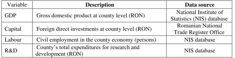
Table 1. Variables for the knowledge production function model

Variable Description Data source

GDP Gross domestic product at county level (RON) National Institute of Statistics (NIS) database

Capital Foreign direct investments at county level (RON) Romanian National Trade Register Office Labour Civil employment in the county economy (persons) NIS database

R&D County’s total expenditures for research and

development (RON) NIS database

We are further going to apply the model of aggregate production functions of

Cobb-Douglas type, including R&D expenditures, in the form of the standard knowledge

production function model:

  

i i i

i AK L R

GDP

(4)

where GDP is the output (Y), α and β stand for the elasticity of output with respect to

capital K and labor L, respectively (α, β> 0), A is a constant, and R represent the R&D

expenditures. R&D is the variable of interest, as it captures the endogenous technological

change that might impact regional economic development.

In order to estimate the model, we are going to use logarithms of the variables, as

follows:

i i i

i

i A K L R

GDPln ln ln ln 

ln

(5)

We are going to estimate the parameters of the production function, annually, for the

period 2001-2011, using county level (NUTS 3) data from the National Institute of Statistics

and from the Romanian National Trade Register Office. Time and space datasets have been

built for GDP, foreign direct investments, employed population, total research and

development expenditures, for the period 2001 to 2011 and the 42 counties of Romania.

Lacking county data on capital, we used foreign direct investments as proxy.

(7)

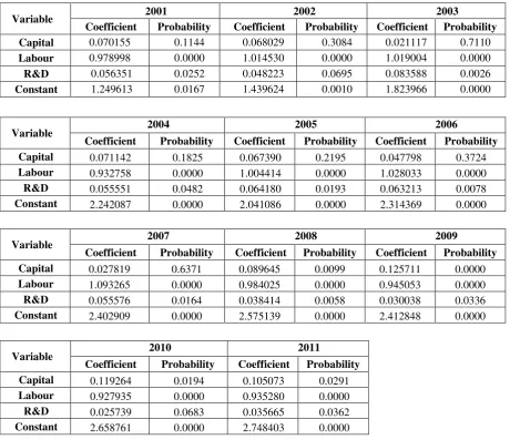
Results of annual parameter estimation of knowledge Cobb-Douglas production function

(Table 2) clearly indicate that endogenous technical progress has had a positive and

statistically significant contribution to regional economic growth in Romania, in every year

[image:7.595.72.533.213.610.2]

of the period under consideration.

Table 2. Annual parameter estimates for knowledge Cobb-Douglas production

function, 2001 to 2011

Variable 2001 2002 2003

Coefficient Probability Coefficient Probability Coefficient Probability Capital 0.070155 0.1144 0.068029 0.3084 0.021117 0.7110

Labour 0.978998 0.0000 1.014530 0.0000 1.019004 0.0000

R&D 0.056351 0.0252 0.048223 0.0695 0.083588 0.0026

Constant 1.249613 0.0167 1.439624 0.0010 1.823966 0.0000

Variable 2004 2005 2006

Labour _0.932758 _0.0000 _1.004414 _0.0000 _1.028033 _0.0000 R&D _0.055551 _0.0482 _0.064180 _0.0193 _0.063213 _0.0078 Constant 2.242087 0.0000 2.041086 0.0000 2.314369 0.0000

Variable 2007 2008 2009

Labour _1.093265 _0.0000 _0.984025 _0.0000 _0.945053 _0.0000 R&D 0.055576 0.0164 0.038414 0.0058 0.030038 0.0336

Constant 2.402909 0.0000 2.575139 0.0000 2.412848 0.0000

Variable 2010 2011

Coefficient Probability Coefficient Probability Capital _0.119264 _0.0194 _0.105073 _0.0291 Labour _0.927935 _0.0000 _0.935280 _0.0000 R&D 0.025739 0.0683 0.035665 0.0362

Constant 2.658761 0.0000 2.748403 0.0000

The results in Table 2 show that labour had the expected positive influence on the county

output and was statistically significant for all years, but the capital (proxied by FDIs) had

been insignificant between 2001 and 2007 and became statistically significant since 2008. It

is likely that FDI (that we only used in absence of other statistical data on capital at the

county level) may not be a suitable option for capturing the production factor capital.

Our results on low but positive impact of R&D on the economic growth in Romania are

(8)

Of special economic interest is the analysis of the parameters of the production function,

as well as the economic policy conclusions arising therefrom. Thus, the estimated parameters

allow measuring the contribution of each input (K, L and R) in creating the output Y with the

following relations:

- capital’s contribution to growth:

  

 

 ,

- labour’s contribution:

  

 

 ,

- R&D’s contribution:

  

 

 .

Based on the previous formulae, we used the estimated parameters to calculate the average contribution of each production factor to regional GDP, over the period 2001 to

2011, obtaining the following results:

- the production factor labour contributed on average by 90% to GDP creation;

- R&D expenditures explain on average 4.5% of regional GDP;

- the capital (using FDIs as proxy) had a contribution of only 5.5%, which suggests that

FDIs have relatively small effects on regional economic growth in Romania.

The standard statistical tests carried out have validated the model, which has a high

explanatory power (approx. 90%). The high heterogeneity of territorial distribution of the

variables used in the model, especially in the case of FDIs, raised estimation problems. To fix

the problem, we used White Heteroskedasticity-Consistent Standard Errors & covariance while estimating the annual models (Annexes).

In conclusion, the main result from the annual estimations of the knowledge production

function model is the positive and significant, but relatively small, contribution of technical

progress (as captured by R&D expenditures) to regional GDP growth in Romania. This

should be a concern and alert decision makers at national and local level on economic and

social policy mix needed to increase the contribution of technological progress, especially

considering the current international trend towards knowledge society. R&D driven

technological progress - the main factor of modern economic growth - as demonstrated by the

experience of developed countries - should act more strongly in the future regional

development of the Romanian economy.

5. Conclusion

Economic theory states the possibility to increase the competitiveness of regional

economies and to fuel economic growth by capitalizing on local technological potential

which might impact upon businesses.

As the origin of innovations and technological change, research and development is a

(9)

found positive and significant, although relatively small, contribution of R&D expenditures

to regional GDP growth. This calls for improved regional research and development strategy,

able to stimulate balanced territorial distribution of R&D and innovation activities, as well as

a closer link with the business sector, in order to take advantage of the economic growth

potential of regional R&D.

Post-crisis regional programs for development should target diversification of local

economies by boosting private investment in R&D, adequate specialization and performance

of local research, development and innovation systems, stimulation of innovative activities

and technology transfer from universities and research centers to production sector, according

to the business needs of local communities, assistance for the development of innovative

SMEs, financial support for companies so that they can acquire advanced technologies and improve their production activity.

References

Aghion, P. and P. Howitt (1992) “A Model of Growth through Creative Destruction”, Econometrica, pp. 323-351.

Aghion, P. and P. Howitt (1998) Endogenous Growth Theory, Cambridge: MIT Press.

Arrow, K. (1962) “The economic implications of learning by doing”, Review of Economic Studies, vol. 29, pp. 155-73.

Buesa, M. (2010) “The determinants of regional innovation in Europe: A combined factorial and regression knowledge production function approach”, Research Policy 0048-7333, Vol.39, Iss.6, p.722

Cameron, G. and J. Muellbauer (1990) “Knowledge, Increasing Returns, and the UK Production Function”, in Mayes, D. ed. Sources of Productivity Growth in the 1980s, Cambridge: Cambridge University Press.

Cobb, C.W. and P.H. Douglas (1928) “A Theory of Production”, American Economic Review, Vol. 18, pp.139-165.

Drivera, C., Oughtonb, C. (2008) “Dynamic models of regional innovation: Explorations with British time-series data”, Cambridge Journal of Regions, Economy and Society, Vol.1, Iss.2, p.205.

Goschin, Z. (2014) “R&D as an Engine of Regional Economic Growth in Romania”, Romanian Journal of Regional Science, vol. 81, pp. 24-37.

(10)

Griliches, Z. (1980) “Returns to R&D Expenditures in the Private Sector”, in Kendrick, K.W. and Vaccara, B. eds. New Developments in Productivity Measurement, Chicago: University Press.

Griliches, Z. and F., Lichtenberg (1984) “R&D and Productivity Growth at the Industry Level: Is There Still a Relationship?”, in Griliches, Z. ed. R&D, Patents and Productivity, Chicago:University of Chicago Press.

Griliches, Z. and J. Mairesse (1998) Production functions: The search for identification in Econometrics and economic theory in the 20th century: the Ragnar Frisch Centennial Symposium, Cambridge University Press, pp. 169-203.

Grossman, T. and E. Helpman (1991) Innovation and Growth in the Global Economy, MIT Press.

Hicks, J.R. (1932) The Theory of Wages, Second Edition 1963, St Martin’s Press, New York.

Kaldor, N. and J. Mirrlees (1962) A New Model of Economic Growth, Review of Economic Studies, pp. 174-245.

Kiefer D.M. (1964) “Winds of Change in Industrial Chemical Research”, Chemical and Engineering News, vol. 42, pp. 88-109.

Lichtenberg, F., R. (1995) The Output Contributions of Computer Equipment and Personal: A Firm-Level Analysis. Economics of Innovation and New Technology 3, pp. 201–217.

Lucas, R. (1988) “On the Mechanics of Economic Development”, in Journal of Monetary Economics, Vol. 22 1, pp.3-42.

Mairesse, J. (1978) “New estimates of embodied and disembodied technical progress”,

Annales de l’INSEE, 30-31, pp.681-720.

Mansfield, E. (1971) “Social and Private Rates of Return from Industrial Innovations”, Quarterly Journal of Economics, vol.91.

Nae, G.G., Sima, C., Economic Growth at Regional Level and Innovation: Is There Any Link?, Annals of the University of Petroşani, Economics, 131, 2013, 149-156, http://www.upet.ro/annals/economics/pdf/2013/part1/Grigore-Sima.pdf

National Institute of Statistics 2013, Database TEMPO - time series, https://statistici.insse.ro/shop/

Romanian National Trade Register Office, Companies by FDI. Statistical Synthesis of the

National Trade Register’s Data, www.onrc.ro/

(11)

Romer, P., M. (1990) “Endogenous Technological Change”, Journal of Political Economy vol. 98, pp. S71-S102.

Solow, R. (1957) “Technical Change and the Aggregate Production Function”, Review of Economics and Statistics, vol. 39, pp. 312-20.

Silaghi M, Medeşfălean R. (2014) “Some insights about determinants of economic growth in Romania. An empirical exercise”, Theoretical and Applied Economics, No. 6, pp. 23-36

Stiglitz, J. (1992) Endogenous Growth and Cycles, Stanford University Working Paper.

Swan, T. (1956) “Economic Growth and Capital Accumulation”, Economic Record, vol. 32, pp. 343-61

Zaman, G., Goschin, Z. (2007a) “Analysis of Macroeconomic Production Functions for Romania. Part one- the time-series approach”, Economic Computation and Economic Cybernetics Studies and Research, no. 1-2, vol.41, pp. 31-46.

Zaman, G., Goschin, Z. (2007b) “Analysis of Macroeconomic Production Functions for Romania. Part two- the cross-section approach”, Economic Computation and Economic Cybernetics Studies and Research, no 3-4, vol.42, pp. 23-32.

(12)

Annexes

Estimations from Cobb-Douglas production function including R&D, annually,

2001-2011

2001

Dependent Variable: LOG(GDP_1) Included observations: 42

White Heteroskedasticity-Consistent Standard Errors & Covariance

Variable Coefficient Std. Error t-Statistic Prob.

LOG(ISD_1) 0.070155 0.043418 1.615806 0.1144

LOG(PO_1) 0.978998 0.105023 9.321703 0.0000

LOG(RD_1) 0.056351 0.024188 2.329733 0.0252

C 1.249613 0.499265 2.502905 0.0167

R-squared 0.896303 Mean dependent var 7.700897

Adjusted R-squared 0.888116 S.D. dependent var 0.585227 S.E. of regression 0.195753 Akaike info criterion -0.333537 Sum squared resid 1.456127 Schwarz criterion -0.168044

Log likelihood 11.00427 F-statistic 109.4840

Durbin-Watson stat 1.823299 Prob(F-statistic) 0.000000

2002

LOG(ISD_2) 0.068029 0.065889 1.032480 0.3084

LOG(PO_2) 1.014530 0.123799 8.194967 0.0000

LOG(RD_2) 0.048223 0.025819 1.867722 0.0695

C 1.439624 0.404581 3.558305 0.0010

2003

(13)

LOG(ISD_3) 0.021117 0.056574 0.373261 0.7110

LOG(PO_3) 1.019004 0.121554 8.383132 0.0000

LOG(RD_3) 0.083588 0.025963 3.219476 0.0026

C 1.823966 0.369009 4.942876 0.0000

2004

LOG(ISD_4) 0.071142 0.052391 1.357897 0.1825

LOG(PO_4) 0.932758 0.088584 10.52968 0.0000

LOG(RD_4) 0.055551 0.027212 2.041412 0.0482

C 2.242087 0.327385 6.848469 0.0000

2005

LOG(ISD_5) 0.067390 0.053983 1.248365 0.2195

LOG(PO_5) 1.004414 0.095893 10.47434 0.0000

LOG(RD_5) 0.064180 0.026275 2.442665 0.0193

C 2.041086 0.339542 6.011286 0.0000

(14)

Log likelihood 14.85479 F-statistic 162.9033 Durbin-Watson stat 1.836456 Prob(F-statistic) 0.000000

2006

LOG(ISD_6) 0.047798 0.052955 0.902621 0.3724

LOG(PO_6) 1.028033 0.103005 9.980379 0.0000

LOG(RD_6) 0.063213 0.022483 2.811533 0.0078

C 2.314369 0.317979 7.278366 0.0000

2007

LOG(ISD_7) 0.027819 0.058503 0.475520 0.6371

LOG(PO_7) 1.093265 0.109485 9.985532 0.0000

LOG(RD_7) 0.055576 0.022138 2.510424 0.0164

C 2.402909 0.346065 6.943527 0.0000

2008

(15)

LOG(PO_8) 0.984025 0.073496 13.38889 0.0000

LOG(RD_8) 0.038414 0.013142 2.923048 0.0058

C 2.575139 0.337103 7.639030 0.0000

2009

LOG(ISD_9) 0.125711 0.024451 5.141311 0.0000

LOG(PO_9) 0.945053 0.072679 13.00319 0.0000

LOG(RD_9) 0.030038 0.013624 2.204771 0.0336

C 2.412848 0.314898 7.662311 0.0000

2010

LOG(ISD_10) 0.119264 0.048840 2.441908 0.0194

LOG(PO_10) 0.927935 0.091306 10.16288 0.0000

LOG(RD_10) 0.025739 0.013719 1.876198 0.0683

C 2.658761 0.410253 6.480785 0.0000

(16)

2011

LOG(ISD_11) 0.105073 0.046332 2.267846 0.0291

LOG(PO_11) 0.935280 0.096466 9.695392 0.0000

LOG(RD_11) 0.035665 0.016428 2.170961 0.0362

C 2.748403 0.482757 5.693135 0.0000