Munich Personal RePEc Archive
A New Factor to Explain Implied
Volatility Smirk
fajardo, José
FGV/EBAPE
31 May 2016
Online at
https://mpra.ub.uni-muenchen.de/71809/
A New Factor to Explain Implied Volatility Smirk
∗Jos´e Fajardo†
May 31, 2016
Abstract
In this paper we find empirical evidence of a new smirk factor, obtained from the
jump structure of the risk neutral distribution of the underlying L´evy process. As an
application we show how to price a barrier style contract.
Keywords: Skewness; L´evy processes; Implied volatility smirk.
JEL Classification: C52; G10
1
Introduction
Since Black and Scholes (1973), many attempts to capture the real behavior of the implied
volatility have been realized. The most well known facts are the volatility smile and smirk, it
shows that depending on moneyness and maturity we can observe a determined behavior. As
for example the fact that out-of-the money put options in equity markets are more expensive
than the corresponding out-of-the money call options, this fact has been extensively address
by many authors, among them we have the work of Foresi and Wu (2005) whom establish the
∗I would like to thank Bruno Dupire, Liuren Wu, Roger Lee and Ernst Eberlein for very useful comments.
I also thank the comments of seminar participants at Stevanovich center University of Chicago. PIMSV– Universitat Bern. IMUB-Universitat de Barcelona. Universit¨at Freiburg. CRM-Universitat Autonoma de Barcelona. V LubraFin. 7th Bachelier Finance Society Meeting and 10th World Congress of The Econometric Society for comments. The usual disclaimer applies.
†Brazilian School of Public and Business Administration. Getulio Vargas Foundation. Praia de Botafogo
above fact for a large data set of option prices for equity indexes in twelve countries. Also,
Carr and Wu (2003) analyze the pattern of implied volatility smirk across maturities using
S&P500 index options. Their findings implies an asymmetric risk neutral distribution for the
index.
On the other hand, the relationship between the implied volatility symmetry and the
mar-ket symmetry, also known as put-call symmetry has been recently established by Fajardo and
Mordecki (2006) and Carr and Lee (2009) for L´evy process and local and stochastic volatility
models, respectively. Also, Fajardo and Mordecki (2014) have shown the relationship among
the skewness premium and the market symmetry parameter. More recently, Fajardo (2015)
has shown how to price some barrier contracts using symmetry properties.
In this paper focusing on pure jump L´evy process with exponential dampening controlling
the skewness we propose a new smirk factor to explain the implied volatility smirk. We test
our specification using S&P500 options data, obtaining a very good fit. Although, there is in
the literature more general data-generating process. including stochastic volatility models, by
focusing on a particular class we can learn a bit more insights about how this particular
pro-cess generates the skew. More exactly, the market symmetry parameter is deeply connected
with the risk neutral excess of kurtosis, which allow us to relate the risk neutral skewness
and kurtosis with the implied volatility skew. In that sense, T´edongap, Feunou, and Fontaine
(2009) also tries to relate skewness and excess kurtosis of the risk neutral distribution with
the skewness of the implied volatility, but instead of suggesting another factor they use a
quadratic model, similar to the one used by Foresi and Wu (2005) but with non constant
parameters.
Also, we show how to price digital call options using our specification. This allow us
moneyness, extending in this ways findings of Fajardo (2015). Although it is well known that
given plain vanilla call or put prices at sufficiently many strikes, the prices of this kind of
barrier contract can be obtained as limits of combinations of such call/put prices, without
needing any model at all. We think that our application can be useful from a practical point of
view since it can help to understand better the relationship between digital call option prices
and implied volatility slopes, and from a regulatory point of view it can be used to compute
probabilities of trigger events, such as the probability of a stock price cross a determined
bar-rier at the end of some given period of time. The calculation of such probabilities are needed
for example in the pricing of some kinds of CoCo bonds, see Schoutens and De Spiegeleer
(2011) for a deep discussion.
The paper is organized as follows. in Section 2 we introduce our model. In Section 3 we
present our specification. In Section 4 we describe our sample. In Section 5 we present the
main results. In Section 6 we present an application and last section concludes.
2
L´
evy Market Model
Consider a real valued stochastic process X = {Xt}t≥0, defined on a stochastic basis B =
(Ω,F,F= (Ft)t≥0,Q), being c`adl`ag, adapted, satisfying X0 = 0 and such that for 0≤s < t
the random variableXt−Xs is independent of the σ-field Fs, with a distribution that only
depends on the difference t−s. Assume also that the stochastic basis B satisfies the usual
conditions (see Jacod and Shiryaev (1987)). The process X is a L´evy process, and is also
called a process with stationary independent increments. For general reference on L´evy
pro-cesses see Jacod and Shiryaev (1987). Skorokhod (1991). Bertoin (1996). Sato (1999). For
L´evy process in Finance see Boyarchenko and Levendorski˘i (2002), Schoutens (2003) and
Cont and Tankov (2004).
formula, that states
EeiqXt = expnthiaq
−12σ2q2+
Z
R
eiqy−1−iqh(y)
Π(dy)io, (1)
with
h(y) =y1{|y|<1},
a fixed truncation function,aandσ ≥0 real constants. and Π a positive measure onR\ {0}1
such thatR
(1∧y2)Π(dy)<+∞, called theL´evy measure. The triplet (a, σ2,Π) is the char-acteristic triplet of the process and completely determines its law.
Consider the set
C0 =nz=p+iq∈C:
Z
{|y|>1}
epyΠ(dy)<∞o. (2)
The set C0 is a vertical strip in the complex plane, contains the line z = iq (q ∈ R), and
consists of all complex numbersz=p+iqsuch thatEepXt <∞for somet >0. Furthermore,
ifz∈C0, we can define the characteristic exponent of the process X. by
ψ(z) =az+1 2σ
2z2+Z
R
ezy−1−zh(y)
Π(dy) (3)
this function ψ is also called the cumulant of X. having E|ezXt| < ∞ for all t ≥ 0, and
EezXt =etψ(z). The finiteness of this expectations follows from Theorem 25.3 in Sato (1999).
Fort= 1, formula (3) reduces to exponent of eq. (1) with Re(z) = 0.
By aL´evy market we mean a model of a financial market with two assets: a deterministic
savings accountB ={Bt}t≥0, with
Bt=ert, r≥0,
whereB0= 1 for simplicity and a stock S={St}t≥0, modelled by
St=S0eXt, S0 =ex>0, (4)
whereX ={Xt}t≥0 is a L´evy process.
In this model we assume that the stock pays dividends, with constant rateδ ≥0, and that
the given probability measureQis the chosen equivalent martingale measure. In other words,
prices are computed as expectations with respect to Q, and the discounted and reinvested
process{e−(r−δ)tSt} is aQ-martingale.
In terms of the characteristic exponent of the process this means that
ψ(1) =r−δ, (5)
based on the fact that Ee−(r−δ)t+Xt = e−t(r−δ−ψ(1)) = 1, and condition (5) can also be
formulated in terms of the characteristic triplet of the process X as
a=r−δ−σ2/2−
Z
R
ey−1−1{|y|<1}
Π(dy). (6)
Then,
ψ(z) =z(r−δ−σ
2
2 ) +z 2σ2
2 +
Z +∞
−∞
[z(1−ey) + (ezy−1)]Π(dy) (7)
Henceforth, we denote this exponent by ψβ due to its future dependence on parameter β of
2.1 Market Symmetry
Here we use the symmetry concept introduced in Fajardo and Mordecki (2006). We define a
L´evy market to besymmetric when the following relation holds
L e−(r−δ)t+Xt |Q
=L e−(δ−r)t−Xt |Q˜
, (8)
meaning equality in law. Here ˜Qis defined by dQ˜t =exdQt. where ˜Qt and Qt denotes the
restrictions of ˜Q and Qto Ft, respectively. As Fajardo and Mordecki (2006) pointed out, a
necessary and sufficient condition for (8) to hold is
Π(dy) =e−yΠ(−dy). (9)
In L´evy markets with jump measure of the form
Π(dy) =eβyΠ0(dy). (10)
where Π0(dy) is a symmetric measure, i.e. Π0(dy) = Π0(−dy) and β is a parameter that
describe the asymmetry of the jumps, everything with respect to the risk neutral measureQ.
As a consequence of (9). Fajardo and Mordecki (2006) found that the market is
symmet-ric if and only ifβ =−1/2.
Recently, De Oliveira, Fajardo, and Mordecki (2015) and Gerhold and G¨ul¨um (2014)
proved thatβ ≷−1/2⇔ ∂σimp(0,β)
∂x ≷0, locally (any maturity) and globally (small maturity),
3
New Smirk Factor
The quadratic implied volatility approximation presented by Foresi and Wu (2005) and Zhang
and Xiang (2008) test the below quadratic approximation2.
σimp(xi) =γ0+γ1di+γ2d2i +ei, (11)
where di = xi
¯
σ√T,is the standarized moneyness, ¯σ is an average volatility and ei is a normal
distributed error. They called γ0, γ1 and γ2, level, slope and curvature, respectively. We
introduce a new factor that we calltorsion3 and propose to test the following specification:
σimp(xi) =γ0+γ1di+γ2d2i +γ3(di+ 1)β+0.5+ei, (12)
With this specification we capture previous findings that relate the at-the-money
volatil-ity slope with theβ−0.5 sign, when γ1 = 0 and γ3 >0.
Also, to avoid negative values with squares exponents we consider only options with
d >−1.
4
Sample
To test our specification we use options on SP500 from Bloomberg quoted on a randomly
picked date 12/01/2011. To estimate the quadratic curve proposed by Zhang and Xiang
(2008), the lowest strike is selected from the first out-of-the-money put with non-zero bid
price. The highest price is selected from the first out-of-the-money call with non-zero bid
price, see Table (1). Also, the call and put prices are the mid-value of closing bid and ask
2Henceforth FW.
3The intuition for this name cames from the fact that when we plot implied volatility vs. moneyness and
−10 0
10 20
30
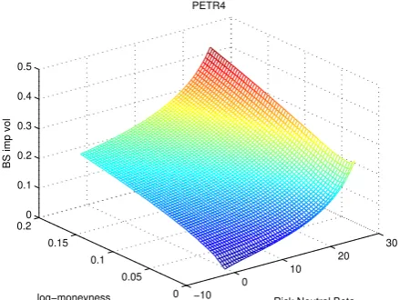
0 0.05 0.1 0.15 0.2
0 0.1 0.2 0.3 0.4 0.5
Risk Neutral Beta PETR4
log−moneyness
[image:9.595.181.401.268.433.2]BS imp vol
Figure 1: BS implied vol vs. Log-moneyness vs. Risk Neutral Beta
prices. The closing index on 12/01/2011 was S0= 1.444.23.
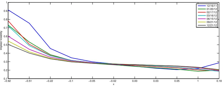
We use the closing VIX of 12/01/20114, as a proxy for the average volatility that is
¯
σ= 27.41%. The resulting implied volatility term structure is presented in figure (2).
−0.92 −0.51 −0.22 −0.1 −0.05 −0.02 0.00 0.03 0.05 1 0.18
0.1 0.2 0.3 0.4 0.5 0.6 0.7 0.8 0.9 1
x
Implied Volatility
[image:10.595.116.476.201.343.2]12/16/11 01/20/12 02/17/12 03/16/12 06/15/12 09/21/12 12/21/12
Figure 2: Implied Volatility Term Structure
For each maturity, the implied forward price F0 is determined based on at-the-money
option price using the following formula
F0 =Strike price+exp(rT)(Call price−P ut price)
wherer is the interest risk-free rate determined by the U.S. treasury bill yield curve rates on
December 1, 2011. A linear extrapolation technique is used to calculate the relevant rate for
the different maturities. The resulting sample is presented in Table (2) below.
[Table (2) about here]
Remember that in order to include the torsion factor we will need to restrictdto be higher
than -1, resulting in less options as presented in Table (3). In FW case it is not necessary.
[Table (3) about here]
5
Results
The Market Symmetry parameter (β) was estimated for two particular processes: the normal
inverse Gaussian (NIG) and the generalized hyperbolic (GH) process, we made this choice
since these models have shown a very good fit with financial returns, see Eberlein and Prause
(2002) and Fajardo and Farias (2004). Also, two spans for the daily return (2 and 5 years)
were considered.
We consider daily returns and implied volatilities of S&P500 extracted from Bloomberg.
Then, we consider the sample periods: 12/01/2009 to 12/01/2011 and 12/01/2006 to 12/01/2011.
As, we need the risk-neutral parameters, we use the density given by the Esscher Transform.
To compute this density we need the interest rate so we use the interest rate given by the
U.S. Treasury on that date 12/01/2011. r = 0.0012. Under this transformation we obtain
four possible β, presented in Table (4) below.
[Table (4) about here]
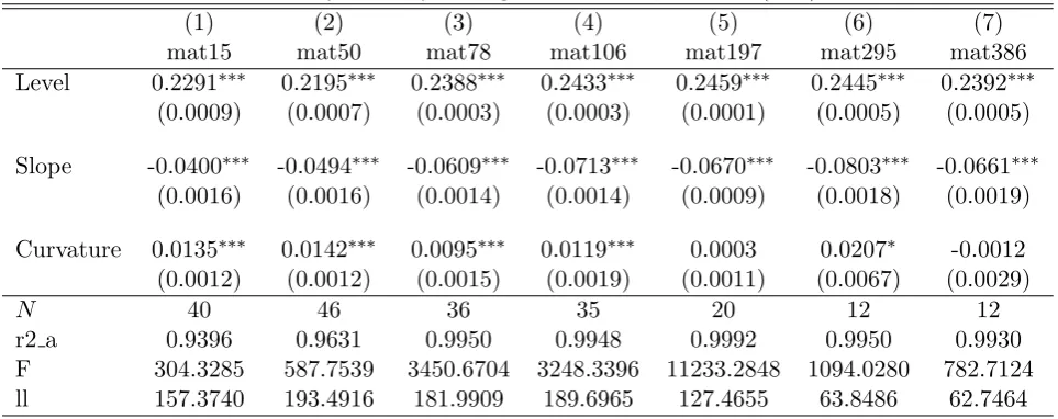
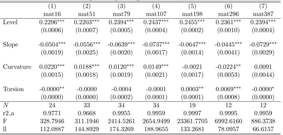
For each maturity we calculate the FW specification and the proposed specification (with
each of the fourβ). For almost all estimatedβ’s the Torsion factor is statistically significant,
mainly for the most liquid maturities, see Tables (5) to (9). Also, the FW model is dominated
in the adjustedR2 criteria by the specifications which include a torsion factor.
5.1 Implied volatility shapes
Now we propose a criteria to choose aβ in terms of more significant values, excellentR2 and
parameter interpretation, for the most liquid options. Then we haveβ =−1.998.5 The other
risk-neutral parameters are given by
(µ, α, δ, β) = (0.0016,31.66,0.0089,−1.998). (13)
The resulting implied volatility approximations are given in Table (10).
[Table (10) about here]
Another good choice in terms ofR2 can beβ =−0.0397 estimated for the GH model, but
we loose the interpretation of the factors, for example the first factor can not be understood
as a realistic initial level of implied volatility. It is important to mention that we are not
claiming to have the specification with the best fit among all the possible specifications.
6
Application: Digital Call Option
In our L´evy market, introduced in Section 2, consider a European style digital call option
with maturity T and barrier Kx, i.e. at maturity derivative pays off f(y) = 1{ey≥Kx}. We
can takey =XT + log(S0) + (r−δ)T. thenf(XT) = 1{eXT≥ex}.
Now denote by I(β, x) the integral defined by:
I(x, β) =−e−
rT
2π Z
iv+R
eizx1 ize
T ψ(−z)dz.
∀x. v >0. (14)
which is the price of the introduced digital call option at log-moneyness x and symmetry
5It is also important to mention that this choice ofβallow us to guaranteeσ
parameter β. This integral can be computed using Fast Fourier transformation techniques.
Instead we will use the implied volatility approximation presented in this paper, to this end
observe thatI(x, β) =e−rTEQ(1
{XT≥x}) =e−
rTQ(X
T ≥x). Henceforth, we will denote this
price by f0.
In Fajardo (2015) the above integral is computed for the case β = −0.5 and then it is
used as a short-cut to price some barrier style contracts under a particular set of moneyness
and asymmetric dynamics that are transformed into symmetric ones. Here we can consider
any dynamic (anyβ) of our set of L´evy processes without the need of such transformation.
Now let BS denote the price of a call option under Black and Scholes model and V the
respective price under our L´evy market model, then
∂V(x, σimp(x, β))
∂x =
∂BS(Kx, σimp(x, β))
∂x =−N(d2(x))Kxe
−rT+∂BS(Kx, σimp(x, β))
∂σ
∂σimp(x, β)
∂x ,
using the fact that6
∂V(x, σimp(x, β))
∂x =−Kxe
−rTQ(S
T ≥Kx),
and with the BS model vega, we obtain:
e−rTQ(ST ≥Kx) =e−rTN(d2(x))−e−(r−δ)T−x
√
T N′(d1(x))
∂σimp(x, β)
∂x ,
with d1(x) =d2(x) +σimp
√
T and d2(x) =−
x+σ
2
impT
2
σimp
√
T , for shorten notation we use σimp
in-stead ofσimp(x, β). The left hand side is equal to the integral value in (14).
Then using specification (12) we obtain the following approximation for the digital call
option price
6Here we need the law ofS
I(β, x)≈e−rTN(d2(x))−e−(r−δ)T−x−
d1 (x)2 2
¯
γ1+ 2 ¯γ2(
x
¯
σ√T) + (β+ 0.5) ¯γ3( x
¯
σ√T + 1)
β−0.5
, (15)
with ¯γi = σ¯√γi2π, i= 1.2.
Now we can price our call digital options, as jumps are more important for short-maturity
options we obtain the price for the first fourth maturities, the results are presented in Table
(11).
[Table (11) about here]
If we compare the prices obtained using Monte Carlo simulation7 we can see that our prices
produce prices for the first fourth maturities, where the number of options is near to 30,
near to the ones obtained using Monte Carlo simulation. As it is known in the literature the
skew due to jumps is stronger in short maturities8. The comparison of prices for near ATM
contracts is presented in Table (12).
[Table (12) about here]
If we estimate the generalized hyperbolic model (GH) we would have β =−0.0397 and
we have obtained similar results, see Table (13).
[Table (13) about here]
7
Conclusions
We find empirical evidence of a new factor to explain the implied volatility smirk. This new
factor that we calledtorsion factor, considers the skewness observed on the jump risk neutral
distribution. As expected this factor has most of the time a positive impact on the implied
volatility skew.
As an application we show how to use this implied volatility specification to price a
call digital option, from this price it is easy to obtain the probability that the stock price
cross a fixed barrier at the end of a period. It would be interesting to extend this result to
other kind of barriers such as the ones considered by Corcuera, Fajardo, Schoutens, Jonsson,
Spiegeleer, and Valdivia (2014) and Corcuera, Fajardo, Schoutens, and Valdivia (2016) to
model contingent convertibles.
References
Bertoin, J. (1996): L´evy Processes. Cambridge University Press, Cambridge.
Black, F., and M. Scholes (1973): “The Pricing of Options and Corporate Liabilities,”
Journal of Political Economy, 81, 637–659.
Boyarchenko, S., and S. Levendorski˘i (2002): Non-Gaussian Merton-Black-Scholes
Theory. World Scientific, River Edge, NJ.
Carr, P., and R. Lee (2009): “Put Call Symmetry: Extensions and Applications,”Math.
Finance., 19(4), 523–560.
Carr, P., and L. Wu (2003): “Finite Moment Log Stable Process and Option Pricing,”
Journal of Finance, 58(2), 753–777.
Cont, R., and P. Tankov (2004): Financial Modelling with Jump Processes. Chapman &
Hall /CRC Financial Mathematics Series.
Corcuera, J., J. Fajardo, W. Schoutens, H. Jonsson, J. Spiegeleer, and A.
Val-divia (2014): “Close form pricing formulas for Coupon Cancellable CoCos,” Journal of
Corcuera, J., J. Fajardo, W. Schoutens, and A. Valdivia (2016): “CoCos with
Extension Risk. A Structural Approach,” in The Fascination of Probability, Statistics and
their Applications. In Honour of Ole E. Barndorff-Nielsen, ed. by M. Podolskij, R. Stelzer,
S. Thorbjørnsen,and A. Veraart, pp. 447–464. Springer.
De Oliveira, F., J. Fajardo, and E. Mordecki (2015): “Implied Volatility Smirk in
L´evy Market,” Preprint, Available at http://ssrn.com/abstract=2544108.
Eberlein, E., and K. Prause (2002): “The Generalized Hyperbolic Model: Financial
Derivatives and Risk Measures,” inMathematical Finance-Bachelier Congress 2000, ed. by
S. P. T. V. H. Geman, D. Madan. Springer Verlag.
Fajardo, J. (2015): “Barrier Style Contracts under L´evy Processes: An Alternative
Ap-proach,” Journal of Banking and Finance, 53, 179–187.
Fajardo, J., and A. Farias (2004): “Generalized Hyperbolic Distributions and Brazilian
Data,” Brazilian Review of Econometrics, 24(2), 249–271.
Fajardo, J., andE. Mordecki(2006): “Symmetry and Duality in L´evy Markets,”
Quan-titative Finance, 6(3), 219–227.
(2014): “Skewness Premium with L´evy Processes,” Quantitative Finance, 14(9),
1619–1626.
Foresi, S., and L. Wu (2005): “Crash-O-Phobia: A Domestic Fear or A Worldwide
Con-cern?,” Journal of Derivatives, 13(2), 8.
Gerhold, S., and I. C. G¨ul¨um (2014): “The Small-Maturity Implied Volatility Slope for
L´evy Models,” Preprint, available at http://arxiv.org/abs/1310.3061.
Jacod, J., and A. Shiryaev (1987): Limit Theorems for Stochastic Processes. Springer,
Sato, K.-i. (1999): L´evy Processes and Infinitely Divisible Distributions. Cambridge
Uni-versity Press, Cambridge, UK.
Schoutens, W. (2003): L´evy Processes in Finance: Pricing Financial Derivatives. Wiley,
New York.
Schoutens, W., and J. De Spiegeleer (2011): Contingent Convertible Coco-Notes:
Structuring & Pricing,. Euromoneybooks.
Skorokhod, A. V. (1991): Random Processes with Independent Increments. Kluwer
Aca-demic Publishers, Dordrecht.
T´edongap, R., B. Feunou,andJ.-S. Fontaine(2009): “Implied Volatility And Skewness
Surface,” EFA meeting paper.
Zhang, J., and Y. Xiang (2008): “Implied Volatility Smirk,” Quantitative Finance, 8(3),
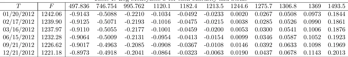
Table 1: Log-Moneynessx for each Maturity and Strike
T F 497.836 746.754 995.762 1120.1 1182.4 1213.5 1244.6 1275.7 1306.8 1369 1493.5
01/20/2012 1242.06 -0.9143 -0.5088 -0.2210 -0.1034 -0.0492 -0.0233 0.0020 0.0267 0.0508 0.0973 0.1844
02/17/2012 1239.90 -0.9125 -0.5071 -0.2193 -0.1016 -0.0475 -0.0215 0.0038 0.0285 0.0526 0.0990 0.1861
03/16/2012 1237.97 -0.9110 -0.5055 -0.2177 -0.1001 -0.0459 -0.0200 0.0053 0.0300 0.0541 0.1006 0.1876
06/15/2012 1232.28 -0.9064 -0.5009 -0.2131 -0.0954 -0.0413 -0.0154 0.0099 0.0346 0.0587 0.1052 0.1923
09/21/2012 1226.62 -0.9017 -0.4963 -0.2085 -0.0908 -0.0367 -0.0108 0.0146 0.0392 0.0633 0.1098 0.1969
Table 2: Option Data
Maturity T F σAT M
imp r δ
12/16/2011 0.0411 1242.87 24.67% 0.208% 1.619%
01/20/2012 0.1370 1242.06 24.52% 0.344% 1.826%
02/17/2012 0.2137 1239.90 25.58% 0.454% 2.218%
03/16/2012 0.2904 1237.97 26.16% 0.498% 2.328%
06/15/2012 0.5397 1232.28 26.64% 0.540% 2.367%
09/21/2012 0.8082 1226.62 26.52% 0.580% 2.358%
12/21/2012 1.0575 1221.18 26.45% 0.604% 2.370%
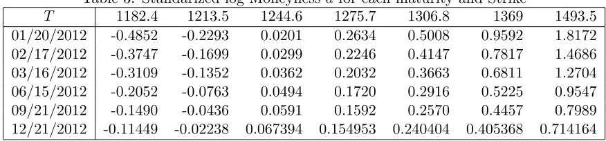
Table 3: Standarized log-Moneyness dfor each maturity and Strike
T 1182.4 1213.5 1244.6 1275.7 1306.8 1369 1493.5
01/20/2012 -0.4852 -0.2293 0.0201 0.2634 0.5008 0.9592 1.8172
02/17/2012 -0.3747 -0.1699 0.0299 0.2246 0.4147 0.7817 1.4686
03/16/2012 -0.3109 -0.1352 0.0362 0.2032 0.3663 0.6811 1.2704
06/15/2012 -0.2052 -0.0763 0.0494 0.1720 0.2916 0.5225 0.9547
09/21/2012 -0.1490 -0.0436 0.0591 0.1592 0.2570 0.4457 0.7989
12/21/2012 -0.11449 -0.02238 0.067394 0.154953 0.240404 0.405368 0.714164
Table 4: Estimated Market Symmetry parameters (β)
5 years 2 years
GH -0.0397 -0.2210
[image:21.595.71.553.235.426.2]NIG -1.998 -4.1792
Table 5: Maturity in x days -Weighted volume. β=−0.5 (FW)
(1) (2) (3) (4) (5) (6) (7)
mat15 mat50 mat78 mat106 mat197 mat295 mat386
Level 0.2291∗∗∗ 0.2195∗∗∗ 0.2388∗∗∗ 0.2433∗∗∗ 0.2459∗∗∗ 0.2445∗∗∗ 0.2392∗∗∗
(0.0009) (0.0007) (0.0003) (0.0003) (0.0001) (0.0005) (0.0005)
Slope -0.0400∗∗∗ -0.0494∗∗∗ -0.0609∗∗∗ -0.0713∗∗∗ -0.0670∗∗∗ -0.0803∗∗∗ -0.0661∗∗∗
(0.0016) (0.0016) (0.0014) (0.0014) (0.0009) (0.0018) (0.0019)
Curvature 0.0135∗∗∗ 0.0142∗∗∗ 0.0095∗∗∗ 0.0119∗∗∗ 0.0003 0.0207∗ -0.0012
(0.0012) (0.0012) (0.0015) (0.0019) (0.0011) (0.0067) (0.0029)
N 40 46 36 35 20 12 12
r2 a 0.9396 0.9631 0.9950 0.9948 0.9992 0.9950 0.9930
F 304.3285 587.7539 3450.6704 3248.3396 11233.2848 1094.0280 782.7124
ll 157.3740 193.4916 181.9909 189.6965 127.4655 63.8486 62.7464
Standard errors in parentheses
Table 6: Maturity in x days -Weighted volume,β =−0.0397
(1) (2) (3) (4) (5) (6) (7)
mat15 mat50 mat78 mat106 mat197 mat295 mat386
Level 0.0928∗∗∗ 0.0669 -0.1476∗ 0.1289 0.3389∗∗∗ 1.7178∗∗∗ 0.1309∗
(0.0183) (0.0338) (0.0585) (0.0747) (0.0531) (0.1908) (0.0493)
Slope -0.1162∗∗∗ -0.1303∗∗∗ -0.2409∗∗∗ -0.1256∗∗ -0.0245 0.6063∗∗∗ -0.1227∗∗
(0.0092) (0.0169) (0.0272) (0.0347) (0.0255) (0.0889) (0.0258)
Curvature 0.0336∗∗∗ 0.0326∗∗∗ 0.0432∗∗∗ 0.0241∗∗ -0.0078 -0.1318∗∗∗ 0.0187
(0.0020) (0.0035) (0.0052) (0.0071) (0.0062) (0.0199) (0.0094)
Torsion 0.1376∗∗∗ 0.1546∗∗∗ 0.3873∗∗∗ 0.1148 -0.0930 -1.4749∗∗∗ 0.1086
(0.0184) (0.0341) (0.0586) (0.0749) (0.0532) (0.1910) (0.0494)
N 24 33 34 34 19 12 12
r2 a 0.9910 0.9796 0.9979 0.9960 0.9996 0.9993 0.9951
F 843.0112 512.0774 5218.5720 2736.0443 15958.7152 5498.9105 745.7024
ll 123.2410 152.9147 187.3914 189.4751 129.6487 76.6545 65.5822
Standard errors in parentheses
∗
p <0.05,∗∗
p <0.01,∗∗∗
p <0.001
Table 7: Maturity in x days -Weighted volume. β =−1.998
(1) (2) (3) (4) (5) (6) (7)
mat15 mat50 mat78 mat106 mat197 mat295 mat386
Level 0.2303∗∗∗ 0.2209∗∗∗ 0.2482∗∗∗ 0.2459∗∗∗ 0.2428∗∗∗ 0.1939∗∗∗ 0.2401∗∗∗
(0.0006) (0.0008) (0.0024) (0.0020) (0.0013) (0.0061) (0.0005)
Slope -0.0520∗∗∗ -0.0572∗∗∗ -0.0764∗∗∗ -0.0766∗∗∗ -0.0618∗∗∗ 0.0021 -0.0740∗∗∗
(0.0019) (0.0027) (0.0040) (0.0036) (0.0029) (0.0099) (0.0034)
Curvature 0.0229∗∗∗ 0.0198∗∗∗ 0.0189∗∗∗ 0.0165∗∗∗ -0.0034 -0.0464∗∗∗ 0.0099
(0.0015) (0.0019) (0.0027) (0.0030) (0.0027) (0.0084) (0.0048)
Torsion -0.0006∗∗ -0.0004 -0.0088∗∗∗ -0.0023 0.0031∗ 0.0490∗∗∗ -0.0007∗
(0.0001) (0.0003) (0.0022) (0.0019) (0.0012) (0.0059) (0.0003)
N 24 33 34 34 19 12 12
r2 a 0.9800 0.9685 0.9966 0.9959 0.9997 0.9994 0.9957
F 376.2852 328.8694 3256.0732 2663.4758 18906.0418 6257.3355 859.9674
ll 113.6776 145.7776 179.3921 189.0198 131.2582 77.4294 66.4348
Standard errors in parentheses
[image:22.595.73.553.455.685.2]Table 8: Maturity in x days -Weighted volume. β =−0.221
(1) (2) (3) (4) (5) (6) (7)
mat16 mat51 mat79 mat107 mat198 mat296 mat387
Level 0.0930∗∗∗ 0.0701 -0.1883∗∗ 0.1195 0.3517∗∗∗ 1.8972∗∗∗ 0.1291∗
(0.0198) (0.0362) (0.0674) (0.0832) (0.0582) (0.2126) (0.0489)
Slope -0.0911∗∗∗ -0.1012∗∗∗ -0.1821∗∗∗ -0.1075∗∗∗ -0.0377∗ 0.3891∗∗∗ -0.1036∗∗∗
(0.0064) (0.0115) (0.0192) (0.0235) (0.0173) (0.0604) (0.0167)
Curvature 0.0312∗∗∗ 0.0297∗∗∗ 0.0387∗∗∗ 0.0226∗∗ -0.0070 -0.1155∗∗∗ 0.0168
(0.0019) (0.0031) (0.0047) (0.0063) (0.0055) (0.0177) (0.0084)
Torsion 0.1373∗∗∗ 0.1513∗∗∗ 0.4280∗∗∗ 0.1242 -0.1058 -1.6544∗∗∗ 0.1104
(0.0200) (0.0365) (0.0676) (0.0833) (0.0583) (0.2128) (0.0490)
N 24 33 34 34 19 12 12
r2 a 0.9898 0.9781 0.9978 0.9960 0.9996 0.9993 0.9952
F 745.6018 476.9556 4964.7221 2725.0741 16169.0434 5567.6743 759.6918
ll 121.7798 151.7648 186.5453 189.4070 129.7730 76.7290 65.6934
Standard errors in parentheses
∗
p <0.05. ∗∗
p <0.01. ∗∗∗
p <0.001
Table 9: Maturity in x days -Weighted volume. β =−4.1792
(1) (2) (3) (4) (5) (6) (7)
mat16 mat51 mat79 mat107 mat198 mat296 mat387
Level 0.2296∗∗∗ 0.2203∗∗∗ 0.2394∗∗∗ 0.2437∗∗∗ 0.2455∗∗∗ 0.2361∗∗∗ 0.2394∗∗∗
(0.0006) (0.0007) (0.0005) (0.0004) (0.0002) (0.0010) (0.0004)
Slope -0.0504∗∗∗ -0.0556∗∗∗ -0.0639∗∗∗ -0.0737∗∗∗ -0.0647∗∗∗ -0.0445∗∗∗ -0.0729∗∗∗
(0.0019) (0.0025) (0.0020) (0.0017) (0.0014) (0.0041) (0.0029)
Curvature 0.0220∗∗∗ 0.0188∗∗∗ 0.0120∗∗∗ 0.0149∗∗∗ -0.0021 -0.0224∗∗ 0.0091
(0.0015) (0.0018) (0.0019) (0.0021) (0.0017) (0.0053) (0.0044)
Torsion -0.0000∗∗ -0.0000 -0.0004 -0.0001 0.0003∗∗ 0.0069∗∗∗ -0.0000∗
(0.0000) (0.0000) (0.0002) (0.0001) (0.0001) (0.0008) (0.0000)
N 24 33 34 34 19 12 12
r2 a 0.9771 0.9668 0.9955 0.9959 0.9997 0.9995 0.9959
F 328.7946 311.1946 2414.5261 2654.9499 23361.7705 6992.6160 886.3738
ll 112.0887 144.8929 174.3269 188.9655 133.2681 78.0957 66.6157
Standard errors in parentheses
[image:23.595.73.555.455.685.2]Table 10: Implied Volatility Approximations for each Maturity and Log-Moneyness
T 1182.4 1213.5 1244.6 1275.7 1306.8 1369 1493.5
12/16/2011 0.2968 0.2580 0.2298 0.2114 0.2021 0.2087 0.3071
01/20/2012 0.2533 0.2351 0.2198 0.2072 0.1972 0.1842 0.1823
02/17/2012 0.2800 0.2619 0.2459 0.2317 0.2192 0.1990 0.1748
03/16/2012 0.2714 0.2566 0.2431 0.2309 0.2199 0.2011 0.1747
06/15/2012 0.2552 0.2474 0.2398 0.2322 0.2247 0.2100 0.1815
09/21/2012 0.1901 0.1930 0.1949 0.1957 0.1957 0.1931 0.1794
[image:24.595.102.478.336.423.2]12/21/2012 0.2487 0.2418 0.2351 0.2288 0.2228 0.2116 0.1921
Table 11: Call Digital Prices for Different Strikes
K
T 1182.4 1213.5 1244.6 1275.7 1306.8 1369 1493.5
12/16/2011 1.0094 0.5916 0.4119 0.2392 0.1066 0.0113 0.0015
01/20/2012 0.6003 0.4989 0.3923 0.2901 0.1993 0.0685 0.0028
02/17/2012 0.5555 0.4578 0.3720 0.2940 0.2244 0.1116 0.0094
03/16/2012 0.4886 0.4193 0.3520 0.2883 0.2299 0.1315 0.0198
Table 12: Comparison of Digital Call Prices using MC Simulation and Imp. Vol. approxi-mation for near-at-the-money Options
T x IM C Iimpvol
0.0411 0.000587 0.52307 0.4119
0.1370 0.002043 0.45168 0.3923
0.2137 0.003783 0.37546 0.3720
0.2904 0.005341 0.31903 0.3520
Table 13: Digital Call Prices for NIG and GH models
T x Iimpvol(x,−1.998) Iimpvol(x,−0.0397)
0.0411 0.000587 0.4119 0.4073
0.1370 0.002043 0.3923 0.3763
0.2137 0.003783 0.3720 0.4435
[image:24.595.196.386.500.570.2] [image:24.595.143.441.630.704.2]