http://go.warwick.ac.uk/lib-publications
Original citation:
Hadjipantelis, Pantelis Z., Jones, Nick S., Moriarty, John M., Springate, David A. and
Knight, C. G. (Christopher G.). (2013) Function-valued traits in evolution. Journal of The
Royal Society Interface, Vol.10 (No.82). Article: 20121032. ISSN 1742-5689
Permanent WRAP url:
http://wrap.warwick.ac.uk/53788
Copyright and reuse:
The Warwick Research Archive Portal (WRAP) makes the work of researchers of the
University of Warwick available open access under the following conditions.
This article is made available under the Creative Commons Attribution 3.0 Unported (CC
BY 3.0) license and may be reused according to the conditions of the license. For more
details see:
http://creativecommons.org/licenses/by/3.0/
A note on versions:
The version presented in WRAP is the published version, or, version of record, and may
be cited as it appears here.
, 20121032, published 20 February 2013
10
2013
J. R. Soc. Interface
Pantelis Z. Hadjipantelis, Nick S. Jones, John Moriarty, David A. Springate and Christopher G. Knight
Function-valued traits in evolution
Supplementary data
l
http://rsif.royalsocietypublishing.org/content/suppl/2013/02/14/rsif.2012.1032.DC1.htm
"Data Supplement"
References
http://rsif.royalsocietypublishing.org/content/10/82/20121032.full.html#ref-list-1
This article cites 34 articles, 5 of which can be accessed freeThis article is free to access
Subject collections
(216 articles)
biomathematics
(31 articles)
bioinformatics
Articles on similar topics can be found in the following collections
Email alerting service
right-hand corner of the article or click Receive free email alerts when new articles cite this article - sign up in the box at the topherehttp://rsif.royalsocietypublishing.org/subscriptions
rsif.royalsocietypublishing.org
Research
Cite this article:
Hadjipantelis PZ, Jones NS,
Moriarty J, Springate DA, Knight CG. 2013
Function-valued traits in evolution. J R Soc
Interface 10: 20121032.
http://dx.doi.org/10.1098/rsif.2012.1032
Received: 15 December 2012
Accepted: 28 January 2013
Subject Areas:
biomathematics, bioinformatics
Keywords:
comparative analysis, Ornstein – Uhlenbeck
process, non-parametric Bayesian inference,
functional phylogenetics, ancestral
reconstruction, functional Gaussian process
regression
Author for correspondence:
Pantelis Z. Hadjipantelis
e-mail: [email protected]
Electronic supplementary material is available
at http://dx.doi.org/10.1098/rsif.2012.1032 or
via http://rsif.royalsocietypublishing.org.
Function-valued traits in evolution
Pantelis Z. Hadjipantelis
1, Nick S. Jones
2, John Moriarty
3, David A. Springate
4and Christopher G. Knight
41Centre for Complexity Science and Department of Statistics, University of Warwick, Coventry CV4 7AL, UK 2Department of Mathematics, Imperial College London, London SW7 2AZ, UK
3School of Mathematics, and4Faculty of Life Sciences, University of Manchester, Oxford Road,
Manchester M13 9PL, UK
Many biological characteristics of evolutionary interest are not scalar vari-ables but continuous functions. Given a dataset of function-valued traits generated by evolution, we develop a practical, statistical approach to infer ancestral function-valued traits, and estimate the generative evolution-ary process. We do this by combining dimension reduction and phylogenetic Gaussian process regression, a non-parametric procedure that explicitly accounts for known phylogenetic relationships. We test the performance of methods on simulated, function-valued data generated from a stochastic evolutionary model. The methods are applied assuming that only the phylogeny, and the function-valued traits of taxa at its tips are known. Our method is robust and applicable to a wide range of function-valued data, and also offers a phylogenetically aware method for estimating the autocorrelation of function-valued traits.
1. Introduction
The number, reliability and coverage of evolutionary trees are growing rapidly [1,2]. However, knowing organisms’ evolutionary relationships through phylo-genetics is only one step in understanding the evolution of their characteristics [3]. Three issues are particularly challenging. The first is limited information: empirical information is typically available only for extant taxa, represented by tips of a phylogenetic tree, whereas evolutionary questions frequently con-cern unobserved ancestors deeper in the tree. The second is dependence: the available information for different organisms in a phylogeny is independent because a phylogeny describes a complex pattern of non-independence; observed variation is a mixture of this inherited variation and specific variation [4]. The third is high dimensionality: the emerging literature on function-valued traits [5 –7] recognizes that many characteristics of living organisms are best represented as a continuous function rather than a single factor or a small number of correlated factors. Such characteristics include growth or mortality curves [8], reaction norms [9] and distributions [10], where the increasing ease of genome sequencing has greatly expanded the range of species in which distributions of gene [11] or predicted protein [12] properties are avail-able. Therefore, a function-valued trait is defined as a phenotypic trait that can be represented by a continuous mathematical function [9].
Previous work [13] proposed an evolutionary model for function-valued datadrelated by a phylogenyT. The data are regarded as observations of a phylogenetic Gaussian process (PGP) at the tips ofT. That work shows that a PGP can be expressed as a stochastic linear operator X on a fixed set f of basis functions (independent components of variation), so that
d¼XTf: ð1:1Þ
However, the study does not address the linear inverse problem of obtaining estimatesf^ andX^offandX: our first contribution in this paper is to provide an approach to this problem in §2.2 via independent principal component analysis (IPCA; [14]).
We refer toXas themixing matrix, and to the (i,j)th entry ofXas themixing coefficientof theith basis function at thejth taxon. It is these mixing coefficients that we model as evol-ving. For each fixed value ofi, theXijare correlated (owing
to phylogeny) asjvaries over the taxa; the basis functions themselves do not evolve in our model.
In §2.3, we address the problem of estimating the statistical structure of the mixing coefficients by performing phylogenetic Gaussian process regression (PGPR) on each of the rows of ^
X separately. This corresponds to assuming independence between the rows (i.e. that the coefficients of the different basis functions evolve independently). It is commonly argued in the quantitative genetics literature [15] that evolutionary pro-cesses can be modelled as Ornstein–Uhlenbeck (OU) processes. Under these assumptions, the estimation of the for-ward operator reduces to the estimation of a small vectorgof parameters [13]. In §2.1, we clarify the interpretation of these parameters in evolutionary contexts. The explicit PGPR pos-terior likelihood function is then used to obtain maximum-likelihood estimates (MLEs) for g. The estimation of g is known to be a challenging statistical problem [16]. We suggest an approach based on the principle ofbagging[17] in §2.4.
Our final contribution (§2.5) addresses the problem of estimating the function-valued traits of ancestral taxa. The earlier-mentioned PGPR step also returns a posterior distri-bution for the mixing coefficient of each basis function at each ancestral taxon in the phylogeny. At any particular ancestor, the estimated basis functions may be combined stat-istically, using the posterior distributions of their respective mixing coefficients, to provide a posterior distribution for the function-valued trait. Because the univariate posterior distributions are Gaussian, and the mixing is linear, the pos-terior for the function-valued trait has a closed form representation as a GP (equation (2.6)) that provides a major analytical and computational advantage for the approach. We can verify the methods proposed by using a PGP as a stochastic generative model. This simulates corre-lated function-valued traits across the taxa ofT. Given only the phylogeny and the function-valued traits of taxa at its tips, our estimates for f^ and the ancestral functions are then compared with the simulation.
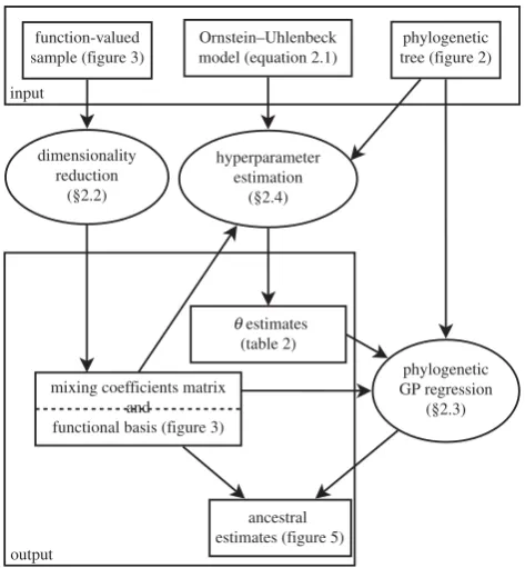
Overall, our three methods (in §§2.2, 2.4, 2.5) appropri-ately combine developments in functional data analysis with the evolutionary dynamics of quantitative phenotypic traits, allowing non-parametric Bayesian inference from phy-logenetically correlated function-valued traits. An outline of the framework presented in this study can be found in figure 1.
2. Methods and implementation
2.1. Artificial evolution of function-valued traits
We begin by generating a random phylogenetic treeTwith 128 tips, shown in figure 2. This fixes the experimental design for our simulation and inference, but further simu-lations given in the electronic supplementary material confirm that the statistical performance of our methods is consistent across a range of choices forT. Branch length dis-tributions are surprisingly consistent across organisms [18]; branch lengths were drawn from the empirical branch length distribution (see electronic supplementary material, section S1) extracted from TREEFAMv. 8.0 [2].Second, we chose a basisfin equation (1.1). We have no reasona priorito suppose that this basis is orthogonal and, in general, there is no reason for our inference procedure to be sen-sitive to the particular shape of the basis functions. The three simple non-orthogonal, unimodal functions shown in figure 3 were therefore chosen as examples. For computational pur-poses, each basis function was stored numerically as a vector of length 1024, so that the basis matrixfwas of size 31024 and itsith row stored theith basis function.
Third, different mixing coefficients were generated by a phylogenetic OU process for each basis function and stored in the respective row of X. Our modelling assumption is that the mixing coefficients for distinct basis functions f1,
f2,f3are statistically independent of each other: in equation (1.1), this means that the rows of X are independent. It is therefore sufficient to describe the stochastic process generat-ingXi, theith row ofXwithi[f1;2;3g. We calculated the
mixing matrix at the 128 tip taxa so X is of size 3128. The ‘true’ ancestral values were established by generating phylogenetic OU processes over the whole phylogeny. The values of this process at tip taxa were stored in a row
function-valued sample (figure 3)
input
Ornstein–Uhlenbeck model (equation 2.1)
phylogenetic tree (figure 2)
dimensionality reduction
(§2.2)
hyperparameter estimation
(§2.4)
q estimates (table 2)
phylogenetic GP regression
(§2.3)
ancestral estimates (figure 5) output
mixing coefficients matrix and
[image:4.595.313.550.40.296.2]functional basis (figure 3)
[image:4.595.316.546.346.485.2]Figure 1.
The three methods presented in this paper (ovals) and their
interrelationships.
Figure 2.
The random phylogenetic tree used and examples of the
function-valued traits shown at the tips (extant taxa) and the internal nodes (ancestral
taxa). A subset of these is used in figure 5.
rsif.r
oy
alsocietypublishing.org
J
R
Soc
Interfa
ce
10:
20121032
vectorXi(Xiis a simulation of the tip taxa mixing coefficientsXi
excluding the non-phylogenetic variation), and its values at internal taxa were stored in a row vectorWifor performance
analyses in §2.5. To simulate the additional effect of non-phylogenetic variation (e.g. due to measurement error or environmental effects), independent (i.e. non-phylogenetic) variation was added to each entry ofXi:
Xi¼Xiþei;
whereeiis a 1128 vector of independent Gaussian errors
with mean 0 and standard deviation si
n; and, finally, the
matrix multiplication in equation (1.1) was performed to obtain the simulated datad. The ‘extant’ function-valued trait at tip taxonjis thusP3i¼1Xijfi(a vector of length 1024), whereas
the ancestral function-valued trait at internal taxon g is
P3
i¼1Wigfi:The ancestral function-valued traits therefore
exhi-bit only the phylogenetic part of simulated variation, whereas the extant function-valued traits exhibit both phylogenetic and non-phylogenetic variation. Of course, it is not possible to reconstruct non-phylogenetic variation using phylogenetic methods: we simulate non-phylogenetic variation only to demonstrate that it does not prevent the reconstruction of the phylogenetic part of variation for ancestral taxa in §§2.2–2.5.
We now comment on the specific parameters chosen for the phylogenetic OU processes mentioned earlier. As in Hansen [19], we refer to thestrength of selection parameter a
and therandom genetic drift s: we add superscripts to these parameters to distinguish between the three different OU processes. With this notation, the mixing coefficients for the rowXihave the following covariance function:
Ki
Tðt1;t2Þ ¼E½XijXig
¼ ðsifÞ2expð2aiDTðtj;tgÞÞ þ ðsinÞ2detj;tg;
ð2:1Þ
wheresi
f¼
ffiffiffiffiffiffiffiffiffiffiffiffiffiffiffiffiffiffiffi
ðsiÞ2=2ai q
;DT(tj,tg) denotes the phylogenetic or
patristic distance (i.e. the distance inT) between thejth and
gth tip taxa,snis defined as earlier, and
detj;tg ¼ 1; iftj¼tgandtjis a tip taxon;
0; otherwise
adds non-phylogenetic variation to extant taxa as discussed earlier, i.e.deevaluates to 1 only for extant taxa, thussn
quan-tifies within-species genetic or environmental effects and measurement error in the ith mixing coefficient. We see from equation (2.1) that the proportion of variation in the rowXiattributable to the phylogeny isðsifÞ2=ðsifÞ2þ ðsinÞ2:
In the Gaussian process regression (GPR) literature in machine learning, 1/2a is equivalent to‘, the characteristic length-scale [20] of decay in the correlation function and in the following we work with the latter. For all of the OU processes, we used characteristic length-scales relative to 8.22, the maximum patristic distance (‘max) between two
extant taxa for our simulated tree (figure 2). The values we used are given in table 1. In particular, sif¼0 when i¼2
−4 −2 0 2 4 6
(a) (b)
(c) (d)
y
−20 −10 0 10 20 30
0 0.2 0.4 0.6 0.8 1.0
x
0 0.2 0.4 0.6 0.8 1.0
x
−4 −2 0 2 4 6
y
[image:5.595.118.482.39.338.2]−4 −2 0 2 4 6
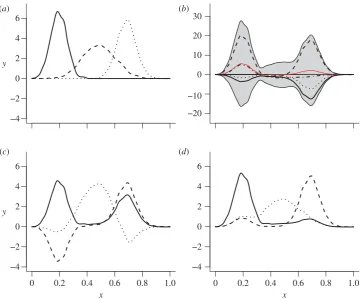
Figure 3.
(
a
) original basis signals,
f
; (
b
) mixed sample at the tips,
d
(four individual function-valued traits are shown; red line and grey band show, respectively,
the mean and 2 s.d. for all 128 function-valued data at the tips); (
d
) IPCA basis,
f
^
; (
c
) PCA basis. (Online version in colour.)
Table 1.
The fixed values used for the parameters in equation (2.1) to
generate the mixing coefficients
X
ij. Each row constitutes a value of
g
i.
6.17 and 2.06 correspond to 0.75 and 0.25 of the tree’s
‘
max, respectively.
When
i
¼
2,
‘
iis not applicable, because there is no phylogenetic
variation in the sample.
i
s
if
‘
i
s
i n1
2.5
6.17
0.5
2
0
n.a.
1.0
3
1.5
2.06
0.5
rsif.r
oy
alsocietypublishing.org
J
R
Soc
Interfa
ce
10:
20121032
[image:5.595.310.556.460.530.2]and it follows that the characteristic length-scale‘ plays no role for this OU process, and equally we do not define the strength-of-selection parameteraiwheni¼2.
2.2. Dimensionality reduction and source separation for
function-valued traits
Given a datasetdof function-valued traits, we would like to find appropriate estimatesX^ andf^ of the mixing matrix X
and the basis setf, respectively. The first task is to identify a good linear subspaceSof the space of all continuous func-tions by choosing basis funcfunc-tions appropriately. The purpose is to work, not with the function-valued data directly, but with their projections inS. We may say that the chosen sub-spaceSis good, if the projected data approximate the original data well, whereas the number of basis functions is not unnecessarily large so that S has the ‘effective’ dimension of the data.
We then face a linear inverse problem: given the datasetd
of function-valued traits, the task is to generate estimates ^
X and f^ (equation (1.1)). This task is also known as source
separation [21], which has a variety of implementations
making different assumptions about the basisf and mixing coefficients X. One widely used approach is principal com-ponents analysis (PCA) [22], which returns orthogonal sets of basis functions to explain the greatest possible variation. PCA has been extended to take account of phylogenetic relationships [23], however, if a sample of functions is gener-ated by mixing non-orthogonal basis functions, the PCs of the sample (whether or not they account for phylogeny) will not equal the basis curves, due to the assumption of orthogon-ality (figure 3). In the independent component analysis (ICA), the alternative assumption is made that the rowsXiofXare
statistically independent. This assumption fits more naturally with our modelling assumptions, because we assume that the rowsXiare mutually independent [21]. ICA has proved
fruitful in other biological applications [24] as has passing the results of PCA to ICA, which has been termed IPCA [14]. PCA is an appropriate tool for identifying the effective dimension of a high-dimensional dataset [25]. Therefore, to achieve both dimension reduction and source separation, we first applied PCA to the dataset d (the 128 function-valued traits at the tips ofT) to determine the appropriate number of basis functions. The PCs were then passed to theCubICA imple-mentation of ICA [26]. CubICA returned a new set of basis functions (figure 3d) that were taken as the estimated basisf^.
2.3. Phylogenetic Gaussian process regression
ICA also returns the estimated mixing coefficients at tip taxa, ^
X: Our next step was to perform PGPR [13] separately on each row X^i;assuming knowledge of the phylogeny T,
in order to obtain posterior distributions for all mixing coefficients throughout the treeT.
GPR [20] is a flexible Bayesian technique in which prior distributions are placed on continuous functions. Its range of priors includes the Brownian motion and OU processes, which are by far the most commonly used models of charac-ter evolution [15,27]. Its implementation is particularly straightforward, because the posterior distributions are also GPs and have closed forms. We now give a brief exposition of GPR, using notation standard in the machine learning literature [20].
A GP may be specified by its mean surface and its covari-ance functionK(g), wheregis a vector of parameters. Because the components ofgparametrize the prior distribution, they are referred to ashyperparameters. The GP prior distribution is denoted
f Nð0;KðgÞÞ:
Ifx* is a set of unobserved coordinates andxis a set of observed coordinates, then the posterior distribution of the vectorf(x*) given the observationsf(x) is
fðxÞjfðxÞ NðA;BÞ; ð2:2Þ
where
A¼Kðx;x;gÞKðx;x;gÞ1fðxÞ; ð
2:3Þ
and
B¼Kðx;x;gÞ Kðx;x;gÞKðx;x;gÞ1Kðx;x;gÞT ð2:4Þ
andK(x*,x,g) denotes thejx*jjxjmatrix of the covariance functionK evaluated at all pairsx
i [X;xj[X:Equations
(2.3) and (2.4) convey that the posterior mean estimate will be a linear combination of the given data and that the pos-terior variance will be equal to the prior variance minus the amount that can be explained by the data. Additionally, the log-likelihood of the samplef(x) is
logpðfðxÞjgÞ ¼ 1
2fðxÞ
TKðx;x;gÞ1fðxÞ
1
2logðdetðKðx;x;gÞÞÞ
jxj
2log 2p: ð2:5Þ It can be seen from equation (2.5) that the MLE is subject both to the fit it delivers (the first term) and the model complexity (the second term). Thus, GPR is non-parametric in the sense that no assumption is made about the structure of the model: the more data gathered, the longer the vectorf(x), and the more intricate the posterior model forf(x*).
PGPR extends the applicability of GPR to evolved func-tion-valued traits. A PGPis a GP indexed by a phylogeny
T, where the function-valued traits at each pair of taxa are conditionally independent given the function-valued traits of their common ancestors. When the evolutionary process has the same covariance function along any branch of T
beginning at its root (called themarginal covariance function), these assumptions are sufficient to uniquely specify the covariance function of the PGP,KT. As we assume thatTis known in our inverse problem, the only remaining modelling choice is therefore the marginal covariance function. As can be seen from equation (2.1),Kis a function of patristic dis-tances on the tree rather than Euclidean disdis-tances as standard in spatial GPR.
In comparative studies, where one has observations at the tips ofT, the covariance functionKTmay be used to con-struct a GP prior for the function-valued traits, allowing functional regression. In the model that we use, this is equiv-alent to specifying a Gaussian prior distribution for the mixing coefficients Yij andXij. This may be carried out by
regarding the row vectorsYiandXias observations of a
uni-variate PGP. As noted in Jones & Moriarty [13], if we assume that the evolutionary process is Markovian and stationary, then the modelling choice vanishes, and the marginal covari-ance function is specified uniquely: it is the stationary OU covariance function. If we also add explicit modelling of non-phylogenetically related variation at the tip taxa, the
rsif.r
oy
alsocietypublishing.org
J
R
Soc
Interfa
ce
10:
20121032
univariate prior covariance function has the unique func-tional form presented in equation (2.1). We do not assume knowledge of the parameters of equation (2.1), however, their estimation is the subject of §2.4.
2.4. Hyperparameter estimation
Because the posterior distributions returned by PGPR depend on the hyperparameter vector g, we must estimate g in order to reconstruct ancestral function-valued traits, and the estimation procedure should correct for the dependence owing to phylogeny. MLE of the phylogenetic variation, non-phylogenetic variation and characteristic length-scale hyperparameterssif;sinand‘i,respectively, may be attempted numerically using the explicit prior likelihood function (equation (2.5)). Because estimatingsifand‘ialone is challen-ging [16] (although the estimation improves significantly with increased sample size), and we have further increased the chal-lenge by introducing non-phylogenetic variation, we propose an improved estimation procedure using the machine learning techniquebagging[17], which a member of theboosting frame-work [22]. We show that these estimates may be further improved if one knows the value of the ratio (sf)2/(sn)2,
which is closely related to Pagel’sl[28].
Bagging (bootstrap aggregating) seeks to reduce the var-iance of an estimator by generating multiple estimates and averaging. It is simple to implement given an existing esti-mation procedure: one adds a loop front end that selects a bootstrap sample and sends it to the estimation procedure and a back end that aggregates the resulting estimates [17]. We generated 100 (sub)trees of 100 taxa by sampling without replacement our original 128 taxa tree, obtained the MLE for
gon each subtree, and averaged these estimates to obtain the aggregated estimateg^:Our results are shown in table 2: for
i¼1 andi¼3, given our moderate sample size (128 taxa), the accuracy of these results is at least in line with the state of the art [16] despite the additional challenge posed by non-phylogenetic variation. For i¼2, where phylogenetic variation is absent from the generative model (sif¼0), our estimation procedure indicates its absence by returning esti-mates for‘iwhose magnitude is unrealistically small for the examined tree (less than the first percentile of the tree’s
patristic distances). Commenting further on this matter, exceptionallysmallcharacteristic length-scales relative to the tree patristic distances, as seen here, practically suggest taxa-specific phylogenetic variation, i.e. non-phylogenetic variation. This holds also in its reverse: exceptionallylarge
characteristic length-scales suggest a stable, non-decaying variation across the examined taxa that is indifferent to their patristic distances, again suggesting the absence of phylogenetic variance among the nodes.
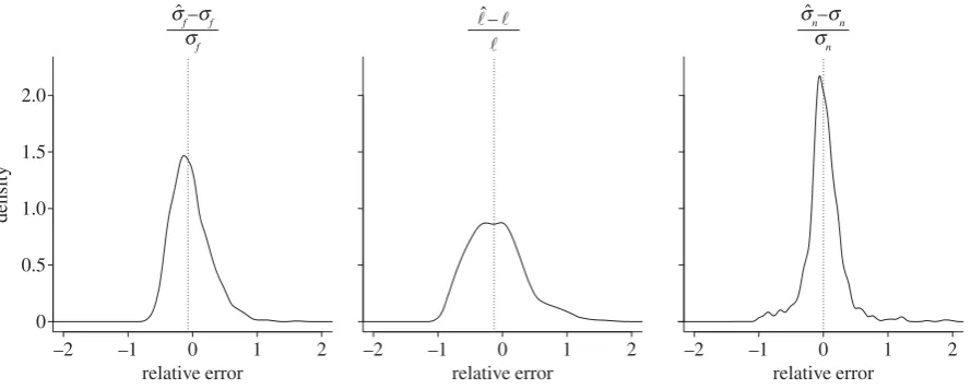
To assess the robustness of this hyperparameter esti-mation method, we performed 1024 simulations, randomly regenerating the tree and parameter vectorg each time (see electronic supplementary material, section S2). The accuracy of these estimates is shown in figure 4. Improved results when the ratio (sf)2/(sn)2 is known a priori (e.g. through
knowledge of Pagel’s l) are also given in the electronic supplementary material, sections S2 and S3. Our ultimate aim is ancestor reconstruction rather than hyperparameter estimationper se, and this is the subject of §2.5.
2.5. Ancestor reconstruction
Having generated function-valued data (§2.1), extracted mixing coefficientsX^ (§2.2) and performed hyperparameter estimation (§2.4), we may now perform PGPR (§2.3) on each rowX^i;to obtain the univariate Gaussian posterior dis-tribution for the mixing coefficientWit at any internal taxon t*. As discussed in §2.3, the GP prior distribution has covari-ance function (equation (2.1)). We have assessed the accuracy
Table 2.
The bagging estimates for the hyperparameters in equation (2.1)
(standard deviations of bagging estimates in parentheses). Each row
corresponds to a given estimate of the vector
g
^
i:
These estimates provide
the maximum-likelihood value for equation (2.5) and are comparable with
the original ones from table 1.
i
s
^
if
‘
^
is
^
ni1
3.41 (0.62)
2.83 (0.47)
0.78 (0.47)
2
0.55 (0.33)
0.05 (0.02)
0.84 (0.34)
3
2.83 (0.33)
2.06 (0.50)
0.73 (0.29)
–2 –1 0 1 2 0.5
1.0 1.5 2.0
relative error
–2 –1 0 1 2 relative error
–2 –1 0 1 2 relative error
density
0
sˆ
f–sf sf
sˆ
n–sn sn
l–l
[image:7.595.78.523.42.220.2]l ˆ
Figure 4.
Kernel density estimates of the relative errors in 1024 runs of the
g
estimation procedure, each time for a different tree, a different set of mixing
coefficients and a different set of parameters in
g
; no components of
g
are assumed to be known beforehand. Estimation results are commented on in §3.
The median values shown by the dotted line are (
2
0.073,
2
0.131 and 0.001), respectively.
rsif.r
oy
alsocietypublishing.org
J
R
Soc
Interfa
ce
10:
20121032
of our bagging estimate g^ in §2.4 and we now substitute ^
gi into equation (2.1). Taking a simple and direct approach,
our estimate f^ obtained in §2.2 may then be substituted into equation (1.1) to obtain the function-valued posterior distribution ft for the function-valued trait at taxon t*.
Because our estimated basis functions are stored numerically as vectors of length 1024, this gives the same discretion for the ancestral traits.
Conditioning on our estimated mixing coefficientsX^ifor
the tip taxa, the posterior distribution ofWit is
Wit NðA^i;B^iÞ;
where the vector A^i and matrix ^Bi are obtained from
equations (2.3) and (2.4), taking x¼X^i; x¼Wit and g^i,
respectively, for our observation coordinates, estimation coor-dinates and hyperparameter vector. Because our prior assumption is that the rows ofXare statistically independent of each other, it follows from equation (1.1) that
ft N
Xk
i¼1
^
Aif^i;Ski¼1f^iTB^if^i !
: ð2:6Þ
The marginal distributions of this representation (mean and standard deviation) are shown in figure 5.
Figure 5 compares the function-valued estimates^ftto the
simulated function-valued traits at the root (figure 5a), an internal node (figure 5b), and at a tip (figure 5c). In figure 5a,b, the simulated function-valued data are shown in black, and can be seen typically to lie within two posterior standard deviations. In figure 5c, the black line is the observed function-valued trait at that tip: the red line and dark grey band represent the posterior distribution of its phy-logenetic component, and the light grey band represents the estimated magnitude of the additional non-phylogenetic variation. Uncertainty over the phylogenetic part of variation (dark grey band) decreases from root to tip, as all obser-vations are at the extant tip taxa. We note that the posterior distributions, even at the root, put clear statistical constraints on the phylogenetic part of ancestral function-valued data: in
this (admittedly simulated and highly controlled) setting, we can reason effectively about ancestral function-valued traits.
3. Discussion
In §2.1, we have appealed to equation (1.1) in the setting of mathematical inverse problems where, given datad, the chal-lenge is to infer a forward operatorGand modelfsuch that
d¼GðfÞ; ð3:1Þ
and such problems are typically under-determined and require additional modelling assumptions [29]. Given a phy-logenyTand function-valued datadat its tips, we wish to infer the forward operatorGTand modelfsuch that
d¼GTðfÞ: ð3:2Þ
When the datadare a small number of correlated factors per tip taxon, a variety of statistical approaches are available [30,31]. When the data are functions, the PGPs [13,32] have been proposed as the forward operator and this is the approach we have taken in this work.
Our dimensionality-reduction methodology in §2.2 can be easily varied or extended. For example, any suitable implementation of PCA may be used to perform the initial dimension reduction step: in particular, if the data have an irregular design (as happens frequently with function-valued data), the method of Yaoet al.[33] may be applied to account for this; the ICA step then proceeds unchanged. We also note that while we find theCubICAimplementation of ICA to be the most successful in our signal separation task, other implementations such asFastICA[21] orJADE[34] can also be used. In general, ICA gives rowsX^iof the estimated
mixing matrix that are maximally independent under a par-ticular measure of independence involving, for example, higher sample moments or mutual information, in order to approximate the solution of the inverse problem in equation (1.1) under our assumption of independence between the rows of X. PCA and ICA have different purposes (respect-ively, orthogonal decomposition of variation and separation
0 0.2 0.4 0.6 0.8 1.0 –10
–5 10
5
0
(a) (b) (c)
x
0 0.2 0.4 0.6 0.8 1.0
x
0 0.2 0.4 0.6 0.8 1.0
[image:8.595.75.534.41.203.2]x y
Figure 5.
Posterior distributions at three points in the phylogeny using the estimated
f
^
and
g
^
. The prediction made by the regression analysis is shown via the
posterior mean (red line), the component of posterior variance due to phylogenetic variation (2 s.d., dark grey band) and non-phylogenetic variation (2 s.d., light
grey band). The black line shows the simulated data enabling visual validation of the ancestral predictions. (
c
), the black line is the training data at a tip taxon the
red line and dark grey band represent the posterior distribution of its phylogenetic component, whereas the light grey band represents the estimated magnitude of
non-phylogenetic variation. The root and internal taxon here are the same as those indicated in figures 2 and 3, and the tip is the second from bottom on the same
figure. (
a
) root estimate; (
b
) node estimate; and (
c
) tip estimate. (Online version in colour.)
rsif.r
oy
alsocietypublishing.org
J
R
Soc
Interfa
ce
10:
20121032
of independently mixed signals) and we use them sequen-tially in IPCA. IPCA is non-parametric and, in particular, both distributionally and phylogenetically agnostic. This means that unlike PCA, IPCA is robust to non-Gaussianity in the data and, unlike phylogenetically corrected PCA, IPCA is robust to mis-specification of the phylogeny and to mixed phylogenetic and non-phylogenetic variation in the data: any of these can be features of biological data.
It can be seen in figure 4 that the estimation of‘is more challenging than the estimation ofsnorsf, having greater
bias and variance. This corresponds to the documented diffi-culty of estimating the parameter a in the OU model, particularly for smaller sample sizes. Our work on hyper-parameter estimation in §2.4 mitigates these difficulties due to small sample size [16,35] by using bagging in order to bootstrap our sample. Somewhat unintuively, bagging ‘works’ exactly because the subsampleg^estimates are vari-able and thus we avoid overfitted final estimates (see electronic supplementary material, section S2). Conceptually, our work on hyperparameter estimation, when taken together with §2.2, relates to the character process models of Pletcher & Geyer [8] and orthogonal polynomial methods of Kirkpatrick & Heckman [5], which give estimates for the autocovariance of function-valued traits. Writing out equation (1.1) for a single function-valued trait (at the jth tip taxon, say), our model may be viewed as
fðxÞ ¼X
3
i¼1
gijfiðxÞ þ
X3
i¼1
eijfiðxÞ; ð3:3Þ
where the mixing coefficient Xij has been expressed as the
sum of gij, the genetic (i.e. phylogenetic) part of variation,
plus eij, the non-phylogenetic (e.g. environmental) part of
variation, just as in these references. Then, the autocorrelation
of the function-valued trait is
E½fðx1Þfðx2Þ ¼
X3
i¼1
ððsfiÞ2þ ðsniÞ2Þfiðx1Þfiðx2Þ: ð3:4Þ
The estimates of sfi and sn
i obtained in §2.4 may be
substituted into equation (3.4) to obtain an estimate of the autocovariance of the function-valued traits under study. This estimate has the attractions both of being positive defi-nite (by construction) and of taking phylogeny into account. Various frameworks exist that could be used to generalize the method presented in §2.4, to model heterogeneity of evol-utionary rates along the branches of a phylogeny [36] or for multiple fixed [15] or randomly evolving [16,37] local optima of the mixing coefficients. For the stationary OU pro-cess, the optimum trait value appears only in the mean, and not in the covariance function, and so does not play a role as a parameter in GPR [20]. We have not implemented such extensions here, effectively assuming that a single fixed opti-mum is adequate for each mixing coefficient. Nonetheless, our framework is readily extensible to include such effects, either implicitly through branch-length transformations [38], or explicitly by replacing the OU model with the more general Hansen model [37].
R code for the IPCA, ancestral reconstruction and hyper-parameter estimation is available from https://github. com/fpgpr/.
P.Z.H. and D.A.S. were supported by an EPSRC Institutional Spon-sorship award to the University of Manchester and the EPSRC Mathematics Platform Engagement activity grant. C.G.K. was sup-ported by a fellowship from the Wellcome Trust. The authors express their gratitude to John A. D. Aston for his encouragement and scientific advice.
References
1. Maddison DR, Schulz KS. 2007The tree of life web project. See http://tolweb.org.
2. Li Het al. 2006 TREEFAM: a curated database of
phylogenetic trees of animal gene families.Nucleic Acids Res.34, D572 – D580. (doi:10.1093/nar/ gkj118)
3. Yang Z, Rannala B. 2012 Molecular phylogenetics: principles and practice.Nat. Rev. Genet.13, 303 – 314. (doi:10.1038/nrg3186)
4. Cheverud JM, Dow MM, Leutenegger W. 1985 The quantitative assessment of phylogenetic constraints in comparative analyses: sexual dimorphism in body weight among primates.Evolution39, 1335 – 1351. (doi:10.2307/2408790)
5. Kirkpatrick M, Heckman N. 1989 A quantitative genetic model for growth, shape, reaction norms, and other infinite-dimensional characters.J. Math. Biol.27, 429 – 450. (doi:10.1007/BF00290638) 6. The Functional Phylogenies Group. 2012
Phylogenetic inference for function-valued traits: speech sound evolution.Trends Ecol. Evol.27, 160 – 166. (doi:10.1016/j.tree.2011.10.001) 7. Stinchcombe JR, Kirkpatrick M, Function-valued
traits working group 2012 Phylogenetic inference for function-valued traits: speech sound evolution.
Trends Ecol. Evol.27, 637 – 647. (doi:10.1016/j.tree. 2012.07.002)
8. Pletcher SD, Geyer CJ. 1999 The genetic analysis of age-dependent traits: modeling the character process.Genetics153, 825 – 835.
9. Kingsolver JG, Gomulkiewicz R, Carter PA. 2001 Variation, selection and evolution of functionvalued traits.Genetica112 – 113, 87 – 104. (doi:10.1023/ A:1013323318612)
10. Zhang Z, Mu¨ller HG. 2011 Functional density synchronization.Comput. Stat. Data Anal.55, 2234 – 2249. (doi:10.1016/j.csda.2011.01.007) 11. Moss SP, Joyce DA, Humphries S, Tindall KJ,
Lunt DH. 2011 Comparative analysis of teleost genome sequences reveals an ancient intron size expansion in the zebrafish lineage.
Genome Biol. Evol.3, 1187 – 1196. (doi:10.1093/ gbe/evr090)
12. Knight CG, Kassen R, Hebestreit H, Rainey PB. 2004 Global analysis of predicted proteomes: functional adaptation of physical properties.Proc. Natl Acad. Sci. USA101, 8390 – 8395. (doi:10.1073/pnas. 0307270101)
13. Jones NS, Moriarty J. 2013 Evolutionary inference or function-valued traits: Gaussian process regression
on phylogenies.J. R. Soc. Interface10, 20120616. (doi:10.1098/rsif.2012.0616)
14. Yao F, Coquery J, Le Cao KA. 2012 Independent principal component analysis for biologically meaningful dimension reduction of large biological data sets.BMC Bioinformatics13, 13 – 24. (doi:10. 1186/1471-2105-13-13)
15. Butler MA, King AA. 2004 Phylogenetic comparative analysis: a modelling approach for adaptive evolution.Am. Nat.164, 683 – 695. (doi:10.1086/ 426002)
16. Beaulieu JM, Jhwueng DC, Boettiger C, O’eara BC. 2012 Modeling stabilizing selection: expanding the Ornstein – Uhlenbeck model of adaptive evolution.
Evolution8, 2369 – 2383. (doi:10.1111/j.1558-5646. 2012.01619.x)
17. Breiman L. 1996 Bagging predictors.Mach. Learn.
24, 123 – 140.
18. Venditti C, Meade A, Pagel M. 2010 Phylogenies reveal new interpretation of speciation and the red queen.Nature463, 349 – 352. (doi:10.1038/ nature08630)
19. Hansen T. 1997 Stabilizing selection and the comparative analysis of adaptation.Evolution51, 1341 – 1351. (doi:10.2307/2411186)
20. Rasmussen CE, Williams CKI. 2006Gaussian processes for machine learning. Cambridge, MA: MIT Press.
21. Hyva¨rinen A, Oja E. 2000 Independent component analysis: algorithms and applications.Neural Netw.13, 411 –430. (doi:10.1016/S0893-6080(00) 00026-5) 22. Bishop C. 2006Pattern recognition and machine
learning. Berlin, Germany: Springer. 23. Revell LJ. 2009 Size-correction and principal
components for interspecific comparative studies.
Evolution63, 3258 – 3268. (doi:10.1111/j.1558-5646.2009.00804.x)
24. Scholz M, Gatzek S, Sterling A, Fiehn O, Selbig J. 2004 Metabolite fingerprinting: detecting biological features by independent component analysis.
Bioinformatics20, 2447 – 2454. (doi:10.1093/ bioinformatics/bth270)
25. Minka TP. 2000 Automatic choice of dimensionality for PCA.Adv. Neural Inf. Process. Syst.13, 514. 26. Blaschke T, Wiskott L. 2004 CuBICA: independent
component analysis by simultaneous third- and fourth-order cumulant diagonalization.IEEE Trans. Signal Process.52, 1250 – 1256. (doi:10.1109/TSP. 2004.826173)
27. Hansen T, Martins E. 1996 Translating between microevolutionary process and macroevolutionary patterns: the correlation structure of interspecific data.Evolution50, 1404 – 1417. (doi:10.2307/ 2410878)
28. Pagel M. 1997 Inferring evolutionary processes from phylogenies.Zool. Scr.26, 331 – 348. (doi:10.1111/j. 1463-6409.1997.tb00423.x)
29. Jaynes ET. 1984 Prior information and ambiguity in inverse problems.Inverse Probl.14, 151 – 166. 30. Salamin N, Wuest RO, Lavergne S, Thuiller W,
Pearman PB. 2010 Assessing rapid evolution in a changing environment.Trends Ecol. Evol.25, 692 – 698. (doi:10.1016/j.tree.2010.09.009)
31. Hadfield JD, Nakagawa S. 2010 General quantitative genetic methods for comparative biology: phylogenies, taxonomies and multi-trait models for continuous and categorical characters.J. Evol. Biol.
23, 494 – 508. (doi:10.1111/j.1420-9101.2009. 01915.x)
32. Kerr M. 2012 Evolutionary inference for functional data: using Gaussian processes on phylogenies of functional data objects. MSc Thesis, University of Glasgow, Glasgow, UK.
33. Yao F, Mu¨ller HG, Wang JL. 2005 Functional data analysis for sparse longitudinal data.J. Am. Stat. Assoc.100, 577 – 590. (doi:10.1198/
016214504000001745)
34. Cardoso JF. 1999 High-order contrasts for independent component analysis.Neural Comput.11, 157 – 192. (doi:10.1162/089976 699300016863)
35. Collar DC, O’Meara BC, Wainwright PC, Near TJ. 2009 Piscivory limits diversification of feeding morphology in centrarchid fishes.Evolution63, 1557 – 1573. (doi:10.1111/j.1558-5646.2009. 00626.x)
36. Revell LJ, Collar DC. 2009 Phylogenetic analysis of the evolutionary coreally using likelihood.Evolution
63 – 64,1090 – 1100. (doi:10.1111/j.1558-5646. 2009.00616.x)
37. Hansen T, Pienaar J, Orzack SH. 2008 A comparative method for studying adaptation to a randomly evolving environment.Evolution8, 1965 – 1977. (doi:10.1111/j.1558-5646.2008.00412.x) 38. Pagel M. 1999 Inferring the historical patterns of
biological evolution.Nature401, 877 – 884. (doi:10. 1038/44766)