An Explicit Solution for a Portfolio Selection Problem with Stochastic Volatility

ISSN Online: 2162-2442 ISSN Print: 2162-2434

An Explicit Solution for a Portfolio Selection

Problem with Stochastic Volatility

Albert N. Sandjo

1

, Fabrice Colin

1

, Salissou Moutari

2

1_{Department of Mathematics & Computer Science, Laurentian University, Sudbury, Canada} 2_{School of Mathematics and Physics, Queen’s University Belfast, Belfast, UK}

Abstract

In this paper, we revisit the optimal consumption and portfolio selection problem for an investor who has access to a risk-free asset (e.g. bank account) with constant return and a risky asset (e.g. stocks) with constant expected re-turn and stochastic volatility. The main contribution of this study is twofold. Our first objective is to provide an explicit solution for dynamic portfolio choice problems, when the volatility of the risky asset returns is driven by the Ornstein-Uhlenbeck process, for an investor with a constant relative risk aversion (CRRA). The second objective is to carry out some numerical expe-riments using the derived solution in order to analyze the sensitivity of the optimal weight and consumption with respect to some parameters of the model, including the expected return on risky asset, the aversion risk of the investor, the mean-reverting speed, the long-term mean of the process and the diffusion coefficient of the stochastic factor of the standard Brownian motion.

Keywords

Portfolio Selection, Stochastic Volatility, Explicit Solution, Ornstein-Uhlenbeck Model, Dynamic Programming Principle

1. Introduction

Portfolio selection is a classical problem in mathematical finance, where the main objective is to seek the best proportion of wealth to invest in risky assets in order to benefit from market opportunities. The derivation of an optimal portfo-lio poses a considerable challenge for market participants because they operate in an uncertain environment. The pioneer work of Markowitz [1][2], who first introduced the so-called mean-variance (MV) model, formulated the portfolio selection problem as an optimization problem, which consists of minimizing the variance (measure of investor’s risk) of the terminal wealth for a desired level of How to cite this paper: Sandjo, A.N.,

Colin, F. and Moutari, S. (2017) An Explicit Solution for a Portfolio Selection Problem with Stochastic Volatility. Journal of Ma-thematical Finance, 7, 199-218.

https://doi.org/10.4236/jmf.2017.71011

Received: January 13, 2017 Accepted: February 25, 2017 Published: February 28, 2017

Copyright © 2017 by authors and Scientific Research Publishing Inc. This work is licensed under the Creative Commons Attribution International License (CC BY 4.0).

http://creativecommons.org/licenses/by/4.0/

expected return. Michaud [3] found that the MV-optimized portfolios are quite unintuitive and difficult for practitioners to implement. Moreover, in a realistic setting, the Markowitz model doesn’t take in account the consumption of the investor.

Another line of research in portfolio optimization is based on the Utility Theory and Expected Utility Maximization, where the preferences of an investor are described by a utility function. In this setting, the objective of the investor is to maximize the expected value of a utility function of the terminal wealth. The combined continuous-time problem of optimal portfolio selection and con-sumption rules was first studied by Merton [4][5], who established the frame-work for dynamic portfolio choice under environmental uncertainty. Using Dy-namic Programming, Merton’s framework leads to a nonlinear partial differen-tial equation (PDE), which is a general and rather complex problem, depending on the process governing the volatility; this aspect makes it difficult to find the optimal weights for the portfolio as well as the corresponding optimal consump-tion. Merton [4] explicitly solved the PDE under a constant volatility of the risk asset.

Recently, there has been a growth of interest in portfolio optimization prob-lems under stochastic volatility. In [6], the authors analyzed the optimal con-sumption and portfolio selection problem, respectively, where the stochastic vo-latility is correlated with the diffusion process of the risky asset, whereas Goll and Kallsen [7] derived explicit solutions for log-optimal portfolios in complete markets in using semi-martingale characteristics of the price process. In [8], the authors established some existence and uniqueness results for the optimal in-vestment problem, for an arbitrage-free model. Chacko and Viceira [9] obtained an exact solution in incomplete markets, when the volatility process is driven by CIR (Cox, Ingersoll and Ross) model [10]. Bae et al. [11] introduced a stock market model with time-varying volatilities coupled with each other via a regime switching mechanism and a constant interaction weighting. A problem similar to the one posed by Merton was analyzed by Brennan and Xia [12][13][14] and Wachter [15] a well as some of the references therein. In [16], Liu established an explicit solution to a dynamic portfolio selection problem, when the returns of the risky asset are driven by a “quadratic process”, which is a Markovian diffu-sion process and where the investor has a constant relative risk averdiffu-sion (CRRA) utility function. In [17], Coulon attempted to numerically solve the Merton model using an iterative process based a finite difference scheme. However, the author acknowledged that the convergence conditions have been investigated, and the proposed algorithm required some fine-tuning of the time discretization to converge.

choice problems, when the volatility of asset returns is driven by the Ornstein- Uhlenbeck process, for an investor with CRRA. Afterwards, we carry out some sensitivity analysis of the optimal weight and consumption with respect to vari-ous parameters of the model, including the expected return on risky asset, the aversion risk of the investors, the mean-reverting speed, the long-term mean of the process and the diffusion coefficient of the stochastic factor of Brownian motion. For the derivation of the explicit solution, unlike in [16], here we pro-vide an alternative to the tensor theory approach, thus making results more ac-cessible to practitioners. The approach proposed in this study, provides a rigor-ous, relatively complete and self-contained treatment of the nonlinear PDE, as well as numerical simulations.

The outline of this paper is as follows. Section 2 presents the derivation of an explicit solution for stock portfolio problem when the stock return volatility is described by the Ornstein-Uhlenbeck model. We derive a closed-form solution for optimal portfolio selection and consumption problems for the investor with CRRA utility. Section 3 is dedicated to some sensitivity analysis of the optimal weight and consumption with respect to various parameters of the model. The effects of the financial parameters have been analyzed and economic interpreta-tions of the optimal portfolio selection and consumption are given. The last sec-tion summarizes our findings and hints on possible improvements and future directions.

2. Consumption and Portfolio Decision

2.1. Model Formulation

In our formulation, a portfolio consists of a risk-free asset (e.g. bank account) and a risky asset (e.g. stock) whose price are driven by geometric Brownian mo-tion.

The risk-free asset is described by

( )

( )

0 0

dS t =rS t d ,t (1)

where S0

( )

t denotes the price of one unit of the risk-free asset at time t and r is the instantaneous rate of return from the risk-free asset, and it is assumed to be constant.

The dynamics of the risky asset is driven by the following equation:

( )

( )

( ) ( ) ( )

1 1 1

dS t =µS t dt V t S t+ dB t ,

(2) where S t1

( )

denotes the price of one share of the risky asset at time t and

( )

dB t is the increment of a Brownian a standard motion. In Equation (2), µ

is the expected return of the risky asset and V t

( )

denotes the instantaneous

variance of the risky asset’s return process. The expected excess return of the risky asset versus the risk-free asset, µ−r, is constant over time.

The log-volatility ln

(

V t

( )

)

follows an Ornstein-Uhlenbeck process

( )

(

)

(

( )

)

( )

d lnV t =κ δ−lnV t dt+σdB_ν t , (3)

Brow-nian motion. The parameter δ _{represents a long-term mean of the process,}

whereas κ is a value of mean-reverting speed, and

σ

corresponds to the dif-fusion coefficient of the stochastic factor dB t

( )

. The logarithms of V t

( )

were

taken in order to avoid negative values of the instantaneous variance of the risky asset.

By applying Itô’s Lemma to Equation (3), while setting f X t

(

( )

)

=eX t( ) with

( )

ln

( )

X t = V t , the proportional changes in the volatility of the Ornstein-

Uhlenbeck process writes as follows:

( )

( )

(

( )

)

( )

2

d

ln d d .

2

V t

V t t B t

V t ν

σ

κ δ σ

 

=_ − + _ +

 

(4)

Following Chacko and Viceira [9], it is assumed that the shocks to precision, dBν, are negatively correlated with the shocks, dB, to the return on risky asset,

i.e. ρ<0. From Equation (4), we can deduce that the instantaneous correlation

between proportional changes in variance and the return of the risky asset return is given by

( )

( )

dB t dBν t =ρd .t

 

 

 (5)

Applying again Itô’s Lemma to Equation (3), by taking f X t

(

( )

,t

)

=X t

( )

eκt

with X t

( )

=lnV t

( )

, and using the identity

{

2 2 ₂

}

eaX eaµX+a σX ,

  =   

where

(

_, 2

)

X X

X ∼ µ σ and a∈, it follows that

( )

exp e

(

ln

( )

0

)

2

(

1 e2

)

,

4 t t

V t V

κ

κ σ

δ δ

κ

− −

 ₋ 

 

= + − +

  _{ }

 

 

 



₍₆₎

and

( )

(

)

₍

₍

_{( )}

₎

₎

(

)

2 2 2 2

Var

1 e 1 e

exp 1 exp 2 e ln 0 .

2 2

t t

t

V t

V

κ κ

κ

σ

σ

δ

δ

κ

κ

− −

−

 

 

 _ − _  _ − _

 

= _{ }− _ + − + _

 _{ }  _{ }

   

 

(7)

The investor starts off with an initial endowment S0

( )

0 =x, S1

( )

0 =y. Let us now assume that there are no transaction costs and no constraints on the structure of the portfolio. In particular, any investor in this market may instan-taneously transfer funds from one account to the other and at no costs. Moreo-ver, the investor may hold short positions of any size in both accounts. In this case, we can reparametrize the problem by introducing new variables, namely the total wealth, W t

( )

=S0

( )

t +S t1

( )

, and the fraction of total wealth held in stock at time t,

( )

( )

( )

1

S t w t

W t

= .

The investor consumes the amount in the bank account at rate c t

( )

.

as defined in the economics literature, e.g. [18], and the investor’s wealth,

( )

W t , at time t changes according to the following stochastic differential equ-ation:

( )

( )

(

( )

)

0

_{( )}

( )

( )

1

_{( )}

( )

( )

0 1

d d

dW t W t 1 w t S t w t S t c t d .t

S t S t

 

=  − + −

 

 

Then, with initial wealth, W

( )

0 =W0, the state equation is given by

( ) (

) ( ) ( )

( ) ( )

( ) ( ) ( ) ( )

( )

0

d d d ,

0 .

W t r w t W t rW t c t t w t W t V t B t

W W x y

µ

 = − + −  +

  



= = +

 (8)

The investor’s objective is to maximize the net expected utility of consump-tion plus the expected utility of terminal wealth. In this study, we use a pow-er-law utility function, which belongs to the CRRA class. The problem of optim-al portfolio selection and consumption rules is then formulated as follows:

( ) ( ), 0

( )

( )

(

)

(

( )

)

max eT t d 1 , ,

c t w t U c t t G W T T

λ

α − α

 _{+ −} 

 



∫



 (9)

subject to the budget constraint (8) and W t

( )

≥0 for all t, where T is the date of death, W T

( )

is the value, at time T, of a trading strategy that finances the consumption,

{ }

c t

( )

_{0≤ ≤t T}, over the period

[ ]

0,T , and G W T

(

( )

,T

)

is a specified bequest valuation function usually assumed to be concave in W T

( )

. Note that the term  in (9), short for 0, is the conditional expectation opera-tor, given that W

( )

0 =W0>0 is known. The utility function U is defined by

( )

c with 1 and 0.

U c

γ

γ γ

γ

= < ≠ (10)

The parameter γ, in Equation (9) is the risk aversion coefficient, which is equivalent to the inverse of the elasticity of intertemporal substitution, whereas

α

and λ _{in Equation (9) respectively denote the relative importance of the}

intermediate consumption and the subjective discount factor. When α=0, the

expected utility depends solely on the terminal wealth, and the problem is then called an asset allocation problem.

2.2. Dynamic Optimization Problem

In this section, we derive expressions for optimal policies. We apply the dynamic programming principle of optimality by rewriting (9) into a dynamic program-ming form. For this aim, we define the indirect utility function, J t W V

(

, ,

)

, as follows:

(

, ,

)

: max _{( ) ( ), t} T e s

(

( )

)

d

(

1

)

(

,

( )

)

, t

c t w t

J t W V = _ α −λU c s s+ −α G T W T _



∫



 (11)

where W t

( )

=W and V t

( )

=V .

Following Merton [4][5], we derive the Hamilton-Jacobi-Bellman (HJB) equ-ation for J:

( ) ( ),

{

(

( )

)

(

)

}

0 max e t , , ,

c t w t U c t J t W V

λ

α −

= + _ _ (12)

(

)

(

)

(

) ( )( )

( )

(

)

_{( )}

₍

₎

(

)

(

)

_{( )}

(

)

2 2

2 2 2

2 2 2 2 2 2 2 , , , , , , : , , , , 1 ln 2 2 , , , , , 2

J t W V J t W V

J t W V w t r W rW c t

t W

J t W V J t W V

w t W V V V

V W

J t W V J t W V

V w t WV

V W V µ σ κ δ σ _ρσ ∂ ∂ = + − + −       _{∂ ∂}   ∂  ∂ + ⋅ + _ − + _ ∂ ∂ _{ } ∂ ∂ + + ∂ ∂ ∂  (13)

with boundary condition:

(

, ,

) (

: 1

)

(

,

( )

)

with

(

,

( )

)

e TW T

( )

.

J T W V G T W T G T W T

γ λ

α

γ

−

= − = (14)

Taking as trial solution

(

)

( )

1

, , : e t , W ,

J t W V K t V

γ γ λ α γ − −

= ⋅_ _ ⋅ (15)

where the function K t V

( )

, needs to be found, we can see that J W V t

(

, ,

)

must satisfy the following partial differential equation:

2

1 0, V

t V VV

K

K K K K

K

+ Ξ + Θ − Γ + Σ + = (16)

where

( )

(

₍

₎

)

( )

(

)

( )

(

)

(

)

( )

2 _{2 2}

2 2

2 2 2

: , : 1 ,

1 2 1 2

: ln , : .

1 2 2

r V

V r V

V

r V

V V V V

µ

γ λ _{γ ρ} σ

γ γ γ

γρσ µ _{κ δ} σ σ

γ

 ₋ 

Ξ = Ξ = ⋅ − +  Γ = Γ = −

− _ − _

−  

Θ = Θ = +_ − + _ Σ = Σ =

− _{ }

(17)

with boundary condition

(

)

1 1 1 ,

K T V α γ

α

− −

 

= _ _ if α ≠0, and where the func-tion K t V

( )

, satisfies

2

0, V

t V VV

K

K K K K

K

+ Ξ + Θ − Γ + Σ =

₍₁₈₎

with boundary condition K T V

(

,

)

=1 whenever α =0.

2.3. Exact Solution of Portfolio and Consumption Rules

In the sequel, we present our main results on an explicit solution for the optimal portfolio. The details on the derivation and the proof of the results can be found in the appendix.

difference scheme to solve the resulting PDE and the author emphasised that the proposed algorithm required some fine-tuning of the discretization parameters to converge.

In order to address the limitations associated with the aforementioned studies, we explicitly solve the Partial Differential Equation (PDE) (16) derived from the Ornstein-Uhlenbeck model. By making an appropriate change of variable, we found that the PDE can be reduced to a much more tractable Riccati Equation (see The Appendix for more details). At a first glance the results in the following propositions may look similar to those in [16]. This doesn’t come as surprise since the Ornstein-Uhlenbeck model is a quadratic process. However, the details of the problem and the method of analysis are substantially different.

The results within the following propositions characterize the optimal con-sumption policy and the optimal portfolio choice.

Proposition 1. Assume that γ <1 and γ ≠0. At time t with 0≤ ≤t T ,

the optimal consumption policy c∗ is given by

( )

_{( )}

,

W c t

K t V

∗ _{= (19)}

and the optimal portfolio choice w∗ is given by

( )

₍

₎

2

(

( )

)

ln ,

, 1

K t V r

w t

V V

µ _ρσ

γ

∗ ₌ − ₊ ∂

∂

− (20)

where the function K t V

( )

, satisfies Equation (16) with the boundary

condi-tion

(

)

1 1 1 ,

K T V α γ

α

− −

 

= _ _ , and Ξ Θ Γ, , and Σ are given in (17) if α≠0 and where the function K t V

( )

, satisfies Equation (18) with the boundary

con-dition K T V

(

,

)

=1 whenever α =0.

Note that Equation (19) and Equation (20) do not represent a complete solu-tion to the model until they have been solved for K t V

( )

, .

The first term,

₍

₎

2

1

r V

µ γ

−

− , in the expression of w t

( )

∗ _{in (20), represents}

weight in the mean-variance efficient portfolio. It is also called the myopic de-mand because this is the portfolio weight for an investor who has only a single period objective or a very short investment horizon. The second term in Equa-tion (20) is the intertemporal hedging demand, which is determined by the co-variance ρσ and the indirect utility function J. The term ρσ selects the

portfolios that have the maximum correlation with the state variable V. The

factor ln

(

K t V

( )

,

)

KV

V K

∂

=

∂ measures the sensitivity of the indirect utility func-

tion to the opportunity set and summarizes the investor’s attitude toward changes in the state variable V.

For the optimal portfolio selection, as well as for an asset allocation problem

i.e. α =0 (no intermediate consumption), we explicitly solve the PDE (16).

weight for the risky asset. The proof of the results is given in the appendix. Proposition 2. Assume that γ <1 and γ ≠0 and let ∆ = Θ + Ξ Σ − Γ2 4

(

)

.

The optimal consumption policy c∗ is given by

( )

_e d t( ) ( )g t

c∗ t =W − −

(21)

and the optimal portfolio choice w t∗

( )

is given by

( )

=

₍

₎

2

( )

1

r

w t d t

V

µ _ρσ

γ

∗ − ₊

−

(22)

with

( )

(

)

( )( ) ( )( )

(

)

(

)

(

(

(

)

)

)

(

(

(

(

)

)

)

)

1 2 1 2 2 2 2 2 2 1

2 2 2

2 2

2 2

e 2

if 0,

1 1 _{1 e}

if 0, 2

1 1

sin 2

if 0,

sin cos 1 1 t T t T V t T d t V

V _{t T}

t T t T t T V

ζ ζ

ζ ζ

ζ ζ

ζ

σ γ ρ

ζ

σ γ ρ

ω ϑ ω

ϑ ω ω ω

σ γ ρ

− −

− −



+

 _{⋅ ∆ >}

 _{ − − }

−

  



 _{Θ −}

 = − ⋅ ∆ =  _{− −}   _{ } − + Θ   _{+ −}

 _{⋅ ∆ <}

 _{ − −  − − −}

  



(23)

where

1,2 , if 0,

2

and if 0.

2 2

V

V V

ζ

ϑ ω

 −Θ ± ∆

= ∆ >

 

Θ −∆

 = − = ∆ <



and the domain of d t

( )

when ∆ <0 is such that tan

(

ω

(

t T

)

)

ω

ϑ

− ≠ _for

every t∈

[ ]

0,T , and

( )

( )

1 1 1

ln Ted s Vd .

t

g t s α γ

α − −  ₋      = _{ +  }   

∫



Finally, in the case α =0, we have g t

( )

=0.

In [17], the author found the following result in the case of a stochastic vola-tility, using a similar utility function.

Proposition 3 ([17]). The optimal management is given by

(

)

_{( )}

(

)

( )

( )

* * 2 , , , , , 1 V W c W V t

F V t

F V t r

w

F V t V µ _ρσ γ  ₌    −  _{= +}  ₋ 

where F V t

( )

, is a solution for the following nonlinear partial differential

equ-ation

2

1 0 V

t V VV

F

F F F F

F

+ Ξ + Θ − Γ + Σ + = (24)

As we have mentioned earlier, without analytical solutions available, Coulon

[17] had to rely on numerical approximations that necessitated a fine tuning of the discretization time. By providing explicit analytical solutions to the problem, we fill this gap.

Corollary 1. Reusing notations from Propositions 2 and 3,the optimal port-folio choice *

w is given by Equation (22) while the optimal consumption

policy *

c is given by Equation (21).

Proof. Use Proposition 2 with 1

2

α = _.

3. Numerical Experiments and Economic Interpretations

In this section we carry out some numerical experiments on the model and ana-lyze the qualitative changes in the solution with respect to shifts in the financial parameters. From Equation (22) and Equation (21), the optimal weight and the optimal consumption, respectively, are not always bounded. However for prac-tical purposes, the quantities need to be bounded. Therefore, in order to high-light the practical features of the model, we consider the following set-up for the numerical experiments, which corresponds to the case without short-selling i.e.

( )

(

(

( ) ( )

)

)

min 1, max e d t g t , 0 ;

c t∗ = W − − (25)

and

( )

(

)

2

( )

min 1, max ,

1

r

w t d t

V

µ

_ρσ

γ

∗ ₌ _  − ₊ _

 

 

 _{ − }

  (26)

where d t

( )

and g t

( )

can be found in Proposition 2.

3.1. Sensitivity of the Optimal Weight and Consumption with

Respect to the Expected Return on the Risky Asset

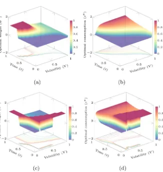
It can be observed that the higher the return of the risky asset, the greater the proportion invested in the risky asset depending on investor risk tolerance. But when the return on the risky asset is smaller than the risk free rate, it is wise to borrow and invest at the risk-free rate, see Figure 1(a) and Figure 1(b). The yields of the risky asset exert a significant impact on investors. The so-called

risk-return trade-off is validated, that is the principle that potential return in-creases as the risk inin-creases. In other words, low levels of uncertainty (low-risk) are associated with low potential returns, whereas high levels of uncertainty (high-risk) are associated with high potential returns. We also observe that higher expected return in the risky asset is likely to lead the consumer to in-crease current consumption and reduce current savings, see Figure 1(c) and

Figure 1(d).

3.2. Sensitivity of the Optimal Weight and Consumption with

Respect to the Return of Risk-Free Asset

[image:10.595.213.539.59.402.2]

Figure 1. Impact the expected return of the risky asset, µ, on the optimal weight ( *

w)

and the optimal consumption (_c*): (a) and (b): µ =₁₅; (c) and (d): µ =₇. The other parameters of the model are set as follows:

5%, 2, 0.25, 1, 3%, 0.5, 5.

r= κ= ρ= − σ = λ= γ= δ=

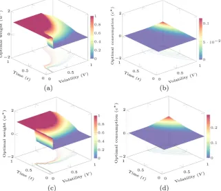
changes in consumption and saving decision of an individual. An increase in the interest rate tends to increase saving and to significantly reduce consumption, see Figure 2. The consumer can achieve any future savings target with a smaller amount of current savings.

3.3. Sensitivity of the Optimal Weight and Consumption with

Respect to the Other Parameters of the Model

In this section, we investigate the impact of the other parameters of the model on the optimal weight and consumption.

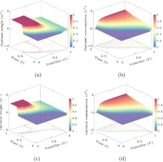
3.3.1. Impact of the Mean-Reverting Speed κ

We observed that the greater the speed of mean reversion in volatility, the great-er the proportion invested in the risky asset for an investor with some risk to-lerance. This proportion is very high at beginning of the period, see Figure 3(a)

Figure 2. Impact the parameter r on the optimal weight ( *

w ) and the optimal

con-sumption (_c*): (a) and (b): _r=_10%; (c) and (d): _r=_5%. The other parameters of the model are fixed as follows: µ=15%, 0.5, 0.25, 1, 3%, 0.95, 5.κ= ρ= − σ= λ= γ= δ=

Figure 3. Impact the parameter κ on the optimal weight ( *

w) and the optimal

con-sumption ( *

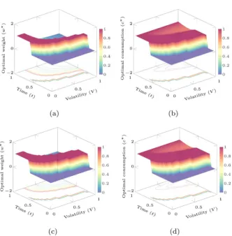
[image:11.595.211.538.68.352.2] [image:11.595.214.536.410.687.2]

3.3.2. Impact of the Diffusion Coefficient of the Stochastic Factor σ

The diffusion coefficient has noticeable effects on the investor. The greater the diffusion coefficient, the greater the proportion invested in the risky asset for an investor with some risk tolerance, see Figure 4(a) and Figure 4(c). By contrast, when the volatility is high, a high risk-averter investor will always choose to in-crease the present consumption, see Figure 4(b) and Figure 4(d).

3.3.3. Impact of the Risk Aversion Coefficient γ

A high risk-averter investor will reduce his/her present consumption if the ex-pected return in the risky asset is high and will invest even more in that asset, see

Figure 5(a) and Figure 5(b). Similarly, a low risk-averter investor will change his/her consumption as the return in the risk-free asset decreases and will also invest more in the risky asset. For a certain degree of relative richness, the in-vestor will give up some present consumption to attain an expected higher re-turn in investment, see Figure 5(c) and Figure 5(d).

3.3.4. Impact of the Correlation Coefficient ρ in the Portfolio

[image:12.595.210.541.360.690.2]

The correlation between the risky assets and the volatility of an individual asset can change and is often negative [9]. An investor may wish to periodically re-

Figure 4. Impact the parameter σ on the optimal weight ( *

w) and the optimal

con-sumption ( *

[image:13.595.212.539.57.402.2]

Figure 5. Impact the parameter γ on the optimal weight ( *

w) and the optimal

con-sumption ( *

c ): (a) and (b): γ = −0.5; (c) and (d): γ=0.5. The other parameters of the model are set as follows: µ=10%, 1%, 2, r= κ= ρ= −0.25, 1, 3%, 5.σ = λ= δ=

balance his/her portfolio to maintain his/her risk exposure and obtain the op-timal level of return on the risky asset. It is observed that the strong negative correlation has an noticeable effect on investment and consumption. In fact, the higher the correlation, the higher the consumption and at the same time, short positions are taken in order to increase investments, see Figure 6.

4. Concluding Remarks

In this study we derive an explicit solution of a model for optimal portfolio se-lection under stochastic volatility. Our main result is a characterization of op-timal portfolio weights and consumption. The major technical difficulties come from the nonlinearity of the model due to the market parameters and con-straints. These difficulties have been overcome using a specific exponential form of the trial solution: a natural theoretical approach is to transform the resulting PDE into a more tractable one, namely a Riccarti equation. After a complete PDE characterization of the value function, we carried out some numerical ex-periments on the model to draw economic interpretations.

[image:14.595.209.542.58.397.2]

Figure 6. Impact the parameter ρ _{on the optimal weight (} *

w) and the optimal

con-sumption (_c*). (a) and (b): ρ = −_0.25; (c) and (d): ρ = −_0.95. The other parameters of the model are set as follows: µ=15%, 5%, 2, 1, 3%, 0.99, 5.r= κ= σ= λ= γ= − δ=

speed, correlation coefficient by examining the consumption decisions of indi-viduals. An important result is the confirmation of the separation theorem proved by Fisher [20] stating that, the portfolio-selection decision is indepen-dent of the consumption decision and the consumption decision is indepenindepen-dent of the financial parameters and only depends upon the level of wealth.

Since the proposed model offers a framework, which is numerically tractable, future work will consider the incorporation of accurate estimate of the model parameters. In particular, risky assets such as stocks depend on parameters that have to be estimated from data. These will provide more specific economic terpretation, depending on the characteristics of the risky assets, enabling to in-vestigate the response of the model not only to predictable events such as divi-dend policy announcements or macroeconomic data releases, but also the con-tagion effect in international markets.

References

[1] Markowitz, H.M. (1952) Portfolio Selection. Journal of Finance, 7, 77-91.

https://doi.org/10.1111/j.1540-6261.1952.tb01525.x

Op-timal? Financial Analysts Journal, 45, 31-42. https://doi.org/10.2469/faj.v45.n1.31

[4] Merton, R.C. (1969) Lifetime Portfolio Selection under Uncertainty: The Conti-nuous-Time Case. The Review of Economics and Statistics, 51, 247-257.

https://doi.org/10.2307/1926560

[5] Merton, R.C. (1971) Optimum Consumption and Portfolio Rules in a Conti-nuous-Time Model. Journal of Economics Theory, 3, 373-413.

https://doi.org/10.1016/0022-0531(71)90038-X

[6] Fleming, W.H. and Hernández-Hernández, D. (2003) An Optimal Consumption Model with Stochastic Volatility. Finance and Stochastics, 7, 245-262.

https://doi.org/10.1007/s007800200083

[7] Goll, T. and Kallsen, J. (2003) A Complete Explicit Solution to the Log-Optimal Portfolio Problem. Annals of Applied Probability, 13, 774-799.

https://doi.org/10.1214/aoap/1050689603

[8] Kramkov, D. and Schachermayer, W. (1999) The Asymptotic Elasticity of Utility Functions and Optimal Investment in Incomplete Markets. Annals of Applied Probability, 9, 904-950. https://doi.org/10.1214/aoap/1029962818

[9] Chacko, G. and Viceira, L.M. (2005) Dynamic Consumption and Portfolio Choice with Stochastic Volatility in Incomplete Markets. Review of Financial Studies, 18, 1369-1402. https://doi.org/10.1093/rfs/hhi035

[10] Cox, J.C., Ingersoll, J.E. and Ross, S.A. (1985) A Theory of the Term Structure of Interest Rates. Econometrica, 53, 385-407. https://doi.org/10.2307/1911242

[11] Bae, H.O., Ha S.Y., Kim, Y., Lee, S.H. and Lim, H. (2015) A Mathematical Model for Volatility Flocking with a Regime Switching Mechanism in a Stock Market. Ma-thematical Models Methods in Applied Science, 25, 1299-1335.

https://doi.org/10.1142/S0218202515500335

[12] Brennan, M.J. and Xia, Y. (2000) Stochastic Interest Rates and Bond-Stock Mix. European Finance Review, 4, 197-210. https://doi.org/10.1023/A:1009890514371

[13] Brennan, M.J. and Xia, Y. (2001) Assessing Asset Pricing Anomalies. Review of Fi-nancial Studies, 14, 905-942. https://doi.org/10.1093/rfs/14.4.905

[14] Brennan, M.J. and Xia, Y. (2002) Dynamic Asset Allocation under Inflation. Journal of Finance, 57, 1201-1238. https://doi.org/10.1111/1540-6261.00459

[15] Wachter, J. (2003) Risk Aversion and Allocation to Long Term Bonds. Journal of Economic Theory, 112, 325-333. https://doi.org/10.1016/S0022-0531(03)00062-0

[16] Liu, J. (2007) Portfolio Selection in Stochastic Environments. The Review of Finan-cial Studies, 20, 1-39. https://doi.org/10.1093/rfs/hhl001

[17] Coulon, J. (2009) Mémoire longue, volatilité et gestion. de portefeuille. Thèse de Doctorat de l’université Claude Bernard-Lyon 1, 1-276.

[18] Bielecki, T.R. and Pliska, S.R. (2003) Economic Properties of the Risk Sensitive Cri-terion for Portfolio Management. Review of Accounting and Finance, 2, 3-17.

https://doi.org/10.1108/eb027004

[19] Heston, S.L. (1993) A Closed-Form Solution for Options with Stochastic Volatility with Applications to Bond and Currency Options. The Review of Financial Studies, 6, 327-343. https://doi.org/10.1093/rfs/6.2.327

Appendix

In the sequel, we provide the details of the proof of Propositions 1 and 2.

Proof of proposition 1. Unlike in [4][5], the volatility under consideration, in our model, is stochastic. Following Merton’s framework [4][5], if we define

(

_{w c W V t}, ; , ,

)

: αe−λt_{U c t}

(

( )

)

_{J t W V}

(

, ,

)

,

Ψ = + _ _ (27)

then the optimality Equation (12) can be rewritten in the following compact form:

( ) ( ),

(

)

max , ; , , 0.

c t w tΨ w c W V t = (28) For the sake of convenience, we respectively denote the derivatives of J with respect to t W, , and V, by

, , ,

t W V

J J J

J J J

t W V

∂ ₌ ∂ ₌ ∂ ₌

∂ ∂ ∂

2 2 2

2 WW, 2 VV and VW.

J J J

J J J

V W

W V

∂ ₌ ∂ ₌ ∂ ₌

∂ ∂

∂ ∂

The first-order conditions for a regular interior extremum

(

c∗

( )

t ,w∗

( )

t

)

to Equation (28) are

(

w c W V t, ; , ,

)

0 e tU c t

(

( )

)

JW,

c

λ

α

∗ ∗ − ∗

∂Ψ _{= = ′ −}

∂ (29)

and

(

)

(

)

( )

2 2 2

, ; , , 0 _{W WW VW}.

w c W V t r J w t W V J WV J

w

µ

ρσ

∗ ∗ ∗

∂Ψ _{= = − + ⋅ + ⋅}

∂ (30)

From Equation (29) and Equation (30), the resulting decision rules for con-sumption and portfolio selection, c∗ and w∗, are given by

( ) ( )

1 e t

W

c t U J

λ

α

−

∗ _{= ′}  

 

  (31)

and

( )

2 .

W VW

WW WW

J J

r w t

J W J V W

µ ρσ

∗ _{= −} − _{⋅ − ⋅}

(32)

Observe that Equation (31) and Equation (32) need to be solved for

(

, ,

)

.

J t W V

Since

(

c∗

( )

t ,w∗

( )

t

)

is an extremum of Ψ

(

w c W V t, ; , ,

)

, substituting the resulting optimal policies, (31) and (32), into (28) yields

(

)

(

( )

)

(

)

(

)

₍

₎

(

)

2 _{2 2 2 2}

2 2

2 2

2

, ; , , 0 e

2 2 ln . 2 2 t t W

W VW W VW

WW WW WW

VV V

w c W V t U c t J rW c J

r J J J J

V r

J J J

V

V J V V J

λ

α

µ ρ σ _{ρσ µ}

σ _{κ δ} σ

∗ ∗ − ∗ ∗

Ψ = = + + −

− − − − −   + + _ − + _   (33)

the CRRA family, that is U c

( )

c

γ

γ

= _with γ <1, γ ≠0 and taking as trial

solu-tion Equasolu-tion (15), that is

(

)

( )

1

, , : e t , W ,

J t W V K t V

γ γ λ α γ − − = ⋅_ _ ⋅

where the function K t V

( )

, needs to be found. Now substituting the conjecture of J into Equation (33), one obtains a necessary condition for J t W V

(

, ,

)

to be a solution to Equation (28). Indeed, after obvious simplifications, J t W V

(

, ,

)

must satisfy the partial differential equation Equation (16) where the coefficients are defined in (17).

Taking into account the fact that

(

, ,

) (

: 1

)

(

,

( )

)

and

(

,

( )

)

e TW T

( )

J T W V G T W T G T W T

γ λ α γ − = − =

we then have the boundary condition

(

)

1 1 1

, .

K T V α γ

α

− −

 

= _ _

Therefore, the consumption (31) and portfolio selection (32) are given by

( )

_{( )}

,

W c t

K t V

∗ _{= (34)}

and

( )

₍

₎

2

(

( )

)

ln ,

1

K t V r w t V V µ _ρσ γ ∗ ₌ − ₊ ∂ ∂

− (35)

This completes the proof of Proposition 1.

Let us now give the proof of Proposition 2. Beyond the simplification of the problem, the main challenge is about solving the PDE (16).

Proof of Proposition 2. Inspired by Liu’s framework [16] who used

( )

_{, e}d t V( )

K t V = as a trial solution, here we chose K t V

( )

, =ed t V( ) +g t( ). Then,

straightforward calculations show that d t

( )

and g t

( )

must satisfy the

iden-tity:

( )

( ) (

) ( )

(

2

)

( )

( ) ( )

, , 1 0

d t V′ + Ξ + Θd t + Σ − Γ d t K t V +g t K t V′ + = (36)

Therefore, a sufficient condition on d t

( )

and on g t

( )

to ensure that

( )

,

K t V is also a solution for Equation (36) is given by

( )

( ) (

) ( )

2

0

d t V′ + Ξ + Θd t + Σ − Γ d t = (37)

and

( ) ( )

, 1 0.

g t K t V′ + =

(38)

In addition, the boundary condition

(

)

1 1 1 ,

K T V α γ

α

− −

 

= _ _ implies that

( )

0

d T = , since the expression doesn’t depend on V . Consequently,

( )

1 1 1

eg T α γ

α

− −

 

=  

  or

( )

1 1

ln 1

g T α

γ α

−

 

= _{ }

solution becomes K t V

( )

, =ed t V( ) and after substitution in Equation (18), we

get

( )

( ) (

) ( )

(

2

)

( )

, 0.

d t V′ + Ξ + Θd t + Σ − Γ d t K t V =

In this case, the boundary condition K T V

(

,

)

=1 implies d T

( )

=0. First step: finding d t

( )

The Riccati Equation (37) can be rewritten in the

form

( )

( )

( )

2

.

d t d t d t V V V

Ξ Θ Γ − Σ

′ = − − +

₍₃₉₎

We perform a variable change to transform Equation (39) into a second order ordinary equation. To do this, we consider a new function F defined by

( )

V F t

_{( )}

( )

.

d t

F t

′ = −

Γ − Σ

Easy algebraic manipulations lead to

(

)

2

0.

V F′′+ ΘVF′− Ξ Γ − Σ F= (40)

It is actually an easy task to solve Equation (40) since we are now facing a second order linear ordinary differential equation.

The characteristic equation of (40) is given by

(

)

2 2

0.

V ζ + ΘVζ − Ξ Σ − Γ = (41)

We then distinguish three cases according to the sign of the discriminant

(

)

2 2

4

D=V _Θ + Ξ Σ − Γ _, which depends upon the term ∆ = Θ + Ξ Σ − Γ: 2 4

(

)

. • _Case: ∆ >0

In this case the roots of the characteristic Equation (41) are real and distinct,

1 et 2 .

2V 2V

ζ =−Θ − ∆ ζ =−Θ + ∆

Therefore, the general solution of (40) is given by

( )

( )1 ( )2

1e 2e

t T t T

F t =c − ζ +c − ζ

where c1 and c2 are real constants and

( )

( )

( ) ( ) ( ) ( ) 1 2 1 2

1 1 2 2

1 2

e e

.

e e

t T t T

t T t T

F t c c F t c c

ζ ζ

ζ ζ

ζ − ζ −

− −

′ +

=

+

The condition d T

( )

=0 implies F T′

( )

=0. Therefore, constants c₁ et c2 satisfy the following conditions c1 1ζ +c2ζ2=0. That is

2

1 2

1

.

c ζ c

ζ

= − _Therefore,

( )

( )

( )( ) ( )( ) 1 2 1 2 2 2 2 1 e = . 1 e t T t T F t F t ζ ζ ζ ζ ζ ζ ζ ζ − − − − ′ + −

• _Case: ∆ =0

and equal. Let’s denote by ζ the common value of ζ1 and ζ2. Then, from (41), we have

2V

ζ

= − Θ _{and the general solution to (40) is given by}

( )

3

(

)

4 exp

(

)

2

F t c t T c T t V Θ   =_ − + _⋅ _ − _   and

( )

3

(

3

(

)

4

)

exp

(

)

.

2 2

F t c c t T c T t

V V

Θ Θ

   

′ =_ − − + _⋅  − 

   

Thanks to the condition F T′

( )

=0, the constants c3 et c4 satisfy the fol-lowing conditions

3 4 with 4 0.

2

c c c V Θ = ≠ Hence,

( )

( )

(

)

(

)

(

)

(

)

(

)

3 3 4

3 4

4 4 4

4 4

2

2 2 2

2

. 2 2

c c t T c F t _V

F t c t T c

c c t T c V V V

c t T c V

t T V V _{t T}

Θ

− − +

′ =

− +

Θ ₋ Θ Θ _{− +} 

    = Θ − + Θ − = − − + Θ

• _Case: ∆ <0

It is clear that the inequality 2

(

)

4

Θ < − Ξ Σ − Γ can only be satisfied if Ξ <0,

since Σ > Γ. This is indeed the case. In fact, due to



(

)

(

)

2 2

2 2 2

1

1 1 1, we have 1 1 0.

2

V

σ

γ ρ ρ γ ρ

<

 

− < − < Σ − Γ = _ − − _>

In this case, the roots of the characteristic equation are complex numbers 2

i with i 1

ζ± = ±ϑ ω = −

where

and .

2V 2V

ϑ= − Θ ω= −∆

The general solution to (40) is then given by

( )

5sin

(

(

)

)

6cos

(

(

)

)

exp

{

(

)

}

, F t =_c ω t−T +c ω t−T _⋅ ϑ t−T

and the derivative of F is

( ) (

5 6

)

cos

(

(

)

)

(

5 6

)

sin

(

(

)

)

exp

{

(

)

}

,

F t′ =_ cω ϑ+ c ω t−T + ϑc −cω ω t−T _⋅ ϑ t−T

where the constants c5 et c6 satisfy the following conditions 6

5 with 6 0.

c

c

ϑ

c

ω

It follows that

( )

6 sin

(

(

)

)

cos

(

(

)

)

exp

{

(

)

}

F t c ϑ ω t T ω t T ϑ t T

ω

 

= _− − + − _⋅ −

 

and

( )

2

(

(

)

)

{

(

)

}

6 sin exp .

F t c ϑ ω ω t T ϑ t T

ω

 

′ = − _ + _ − ⋅ −

 

Thus

( )

( )

(

)

(

)

(

)

(

)

(

)

(

(

)

)

2 2

sin

sin cos

t T F t

F t t T t T

ω

ϑ

ω

ϑ

ω

ω

ω

+ −

′ =

− − −

with the domain of F such that tan

(

ω

(

t T

)

)

ω

ϑ

− ≠ _for 0≤ ≤t T .

Second step: finding g t

( )

Now, Equation (38) leads to

( ) ( )

1 0

eg t = −

∫

te−d s Vds C+ ,

where the constant C1, which can be found using the boundary condition, is given by

( )

1 1

1 ₀

1

e d .

T _{d s V}

C α γ s

α

− ₋

−

 

=_{ } +

 

∫

Finally, the function g t

( )

can be written in the following integral form:

( )

( )

1 1 1

ln Ted s Vd .

t

g t s α γ

α

− −

 ₋ 

 

 

= _{ +  }

 



∫



This completes the proof of Proposition 2.

Submit or recommend next manuscript to SCIRP and we will provide best service for you:

Accepting pre-submission inquiries through Email, Facebook, LinkedIn, Twitter, etc. A wide selection of journals (inclusive of 9 subjects, more than 200 journals)

Providing 24-hour high-quality service User-friendly online submission system Fair and swift peer-review system

Efficient typesetting and proofreading procedure

Display of the result of downloads and visits, as well as the number of cited articles Maximum dissemination of your research work

Submit your manuscript at: http://papersubmission.scirp.org/