Evolutionary, multi-scale analysis of river bank line retreat using
1continuous wavelet transforms: Jamuna River, Bangladesh.
23
4
5
6
Mount, Nick J.1*, Tate, Nicholas J.2, Sarker, Maminul H.3 and Thorne, Colin R.1 7
8
9
* Corr. Auth. [email protected], Tel: +44 (0)115 951 5438, Fax: +44 (0)115 951 15249
10 11
1. School of Geography, University of Nottingham, University Park, Nottingham, NG7 2RD, UK.
12 13
2. Department of Geography, University of Leicester, Leicester, LE1 7RH, UK.
14 15
3. Centre for Environmental and Geographic Information Services, House 6, Road 23/C, Gulshan-1, Dhaka 1212,
16
Bangladesh. 17
Abstract 20
In this study continuous wavelet transforms are used to explore spatio-temporal 21
patterns of multi-scale bank line retreat along a 204 km reach of the Jamuna River, 22
Bangladesh. A sequence of eight bank line retreat series, derived from remotely-sensed 23
imagery for the period 1987-1999, is transformed using the Morlet mother wavelet. 24
Bank erosion is shown to operate at several characteristic spatial and temporal scales. 25
Local erosion and bank line retreat are shown to occur in short, well defined reaches 26
characterised by temporal persistence at the same location, and separated by relatively 27
stable reaches. In contrast, evidence of downstream propagation of bank line retreat 28
patterns is evident at larger spatial scales. The intensity of localised bank line retreat 29
(i.e. at scales of 0 - 20 km) is strongly related to the magnitude of monsoonal peak 30
discharge, but this relationship weakens as the spatial scale of erosion increases. The 31
potential of continuous wavelet analysis to enhancing our understanding of 32
morphological evolution in complex fluvial systems with multi-channel planforms is 33
discussed. 34
Keywords 35
Continuous Wavelet Transform, Jamuna River, Braided river, Time-space, Erosion 36
processes, Embayment pattern, Sediment wave. 37
1. Introduction 38
The planform evolution of the Jamuna River, Bangladesh, the distal portion of the 39
Brahmaputra, has been the focus of many studies in which the aim has been to assess, 40
characterise and quantify the magnitude and distribution of bank line migration (e.g. 41
Coleman, 1969; Sarma and Basumallick, 1984; Singh et al., 1990; Thorne et al., 1993, 42
1995; Thorne and Russell, 1993; Halcrow, 1994; Goswami, 1995; Goswami et al., 1999; 43
Ashworth et al., 2000; CEGIS, 2000, 2007; Khan and Islam, 2003; Sarma and Phukan, 44
2004, 2006; Sankhua et al., 2005; Sarma, 2005; Takagi et al., 2007). However, 45
exhibited by the river are complicated by its large geographical scale (here synonymous 47
with extent) and its complex planform, which features elements of meandering, braiding 48
and anastomosing (Fergusson, 1993). The large geographical scale has thus far 49
precluded the application of well-established hydraulic geometry relationships or 50
process-based explanatory models due to the difficulties associated with up-scaling 51
(Latrubesse, 2008). Furthermore, the river’s complex and dynamic planform has also 52
precluded application of conventional, geometric models developed for simpler, 53
meandering channels (e.g. Ikeda et al., 1981; Parker et al., 1983; Johannesson and 54
Parker, 1989; Zolezzi and Seminara, 2001; Camporeale et al., 2005). In fact, the 55
difficulty inherent in large-scale, long-term studies of channel evolution and bank line 56
migration in complex, multi-channel rivers prior to the wide availability of high definition, 57
remotely sensed imagery explains why such studies have, until recently, been rarely 58
conducted (Best and Bristow, 1993; Richardson, 1997). To date, the majority of 59
geomorphological studies of the Jamuna have instead focused on investigating the 60
processes responsible for channel evolution and bank line migration at the scale of the 61
individual geomorphological unit. Examples include studies of channel bifurcations and 62
braid bars (Ashworth et al., 2000; Richardson and Thorne, 2001); braid bars and 63
associated floodplain embayments (Thorne et al., 1993; Halcrow, 1994) and the 64
evolution of meander bends in major anabranches (Thorne and Russell, 1993; Ellis, 65
1993). 66
The bank line adjustment processes associated with these different 67
geomorphological units exhibit non-stationarity (spatial and temporal localization) as 68
well as different, characteristic bank migration rates and scale-dependency in space 69
(circa 102 - 104 m) and time (circa 100 – 101 yr). It follows that, in rivers with multi-70
channel planforms, the overall pattern of bank retreat is characterized as a complex non-71
stationary waveform within which multiple, characteristic erosion patterns co-exist at 72
different scales, and at different downstream locations. For example, Thorne et al. 73
nodal reaches first described by Coleman (1969) that are spaced along the channel at 75
intervals of circa 30 km. They also identified local bank migration processes that are 76
driven by braid bar growth and migration and which operate at smaller spatial (3 - 6 km) 77
and over shorter temporal scales (2 - 5 years). Their findings contrast with those of Ellis 78
(1993), who observed bank erosion and embayment formation related to meander 79
growth and migration in near-bank anabranches that occur at spatial scales of hundreds 80
of metres to several kilometres, persist over periods of 1-12 years, and drive erosion 81
rates ranging from 50 to over 250 m yr-1. More recently, CEGIS (2007) identified bank 82
erosion and floodplain embayment forming processes associated with bar form 83
development in the Jamuna river operating at spatial scales of 3-15 km, over periods of 84
approximately 15 years and with erosion rates of of the order of 200 m yr-1. A finding 85
common to these studies was that rates of downstream migration in the locations of 86
severe bank erosion also appear to be scale-dependent. This is consistent with the 87
downstream movement of sand bars (Coleman, 1969) and changes in the location of 88
relatively stable and unstable reaches over time (Takagi et al., 2007), which all suggest 89
a link to the downstream propagation of sediment waves (Gilbert, 1917; Madej and 90
Ozaki, 1996; Wathen and Hoey, 1998). Indeed both Thorne et al. (1993) and Takagi et 91
al. (2007) identified wave-like patterns of channel migration, with characteristic 92
wavelengths of ~150 km and ~35 km, respectively. These findings suggest that the 93
complex patterns of bank retreat observed in the Jamuna result from the superimposed 94
and cumulative effects of spatially-transient bank erosion processes, operating semi-95
independently at a range of spatial and temporal scales. 96
Marcus and Fonstad (2010) argue that the development and availability of new 97
remote sensing technologies, coupled with widening accessibility to GIS, have led to the 98
emergence of the ‘remote sensing of rivers’ as a sub-discipline of fluvial geomorphology. 99
Complex patterns of bank migration are now commonly investigated based on temporal 100
sequences of bank line data, captured from aerial photographs or remotely-sensed 101
that rates of bank line retreat during specified periods can be computed (e.g. Gurnell et 103
al., 1994; Mount et al., 2003; Mount and Louis, 2005; Swanson et al., 2011). In such 104
studies, characterisation of downstream migration in bank erosion patterns reduces to a 105
problem of localizing in space the different magnitudes and scales of bank retreat events 106
that can be discerned from the data, and evaluating how these localized patterns vary 107
through time. In the past this has been achieved through a largely qualitative, visual 108
appraisal of the patterns observed in sequential plots of bank position or change (e.g. 109
Downward et al., 1994; Gurnell, 1997; Mount et al., 2003) coupled with examination of 110
summary bank retreat statistics (e.g. CEGIS 2000; 2007). Consequently, relatively little 111
quantitative understanding of either trends in the spatial localization associated with 112
erosion at different scales or the relative rates of erosion driven by the different 113
processes represented in the bank retreat record has been achieved. Moreover, it has 114
been difficult to causally relate the observed patterns of bank retreat to likely 115
geomorphological drivers; especially where these involve processes acting at different 116
spatial and temporal scales. Commenting on this in a recent review, Kleinhans (2010) 117
acknowledged the potential of remotely sensed time-series for unravelling channel 118
pattern changes, but also observed that, ‘we need quantifiers for subtle patterns to 119
reveal structure objectively’ (Kleinhans, 2010; page 313). 120
A more quantitative approach involves viewing the downstream distribution of 121
bank retreat as a spatial signal of planimetric change. According to this approach, the 122
different scales of erosion are equivalent to the different frequencies contained within the 123
signal and their magnitudes are equivalent to signal amplitude. Accordingly, the 124
downstream signal of erosion becomes the spatial equivalent of a standard time series 125
signal, with distance substituted for time. When re-conceptualised in this way, 126
techniques developed for the characterisation of frequency and amplitude in complex 127
signals, become potentially powerful tools for characterising bank retreat. One common 128
tool is the fast Fourier Transform (FFT), which offers good frequency localisation albeit at 129
data series to be consistent with a statistically stationary model – something that cannot 131
necessarily be assumed when analysing bank retreat sequences in river channels (Van 132
Gerven and Hoitink, 2009). Alternative methods offering both frequency and spatial 133
localization, such as the windowed Fourier transform (WFT) (also known as the short-134
time Fourier transform) and wavelet analysis are therefore, preferable. Both have been 135
applied to the analysis of river patterns (Ferguson, 1975; Camporeale et al., 2005, Van 136
Gerven and Hoitink, 2009). However, the WFT is considerably less adaptable than 137
wavelet analysis in that achieving good spatial resolution requires sacrificing frequency 138
localisation, and vice versa (Fournier, 1995 page 11). As a result WFT was not selected 139
for use in this research. While the use of wavelet analysis by geomorphologists remains 140
rare, it has been widely used by hydrologists for the characterisation of runoff time 141
series (e.g. Brillinger, 1994; Fraedrich et al., 1997; Labat et al., 1999, 2000, 2002; 142
Compagnucci et al., 2000; Gaucherel, 2002; Lafreniere and Sharp, 2003; Coulibaly and 143
Burn, 2004; Labat, 2005) Also, its potential in analysing signals in time series of river 144
planform change has recently been recognised by Van Gerven and Hoitink (2009), who 145
used it to characterise meander geometry on the Mahakam River, Indonesia. There are, 146
however, no published examples of its use in characterising bank migration in large 147
rivers with anabranching planforms. 148
In this paper we explore the potential of the continuous wavelet transform (CWT) 149
for the quantitative characterisation of temporal sequences of downstream bank line 150
migration patterns, using data recorded along a 204 km reach of the Jamuna River, 151
Bangladesh. The CWTs presented in this paper quantify changes in bank position in the 152
plane of maximum bank erosion. In line with previous studies of planform change from 153
remotely-sensed data, this is assumed to be orthogonal to the downstream direction. 154
This is believed to be the first time such an approach has been applied in a bank line 155
retreat study. In section 2 we describe the CWT method. Section 3 presents the 156
line retreat on the Jamuna River. The key findings from the study are summarised in 158
section 4. 159
2. Methodology 160
Wavelet analysis comprises several mathematical transforms from which 161
temporal (or spatial) series can be transformed into a 2-D time (or space)-frequency 162
representation. A detailed treatment of the mathematics of wavelet transforms is 163
beyond the scope of this paper, but may be found in publications covering both wavelet 164
analysis theory (see Daubechies, 1992) and software implementation (Nason, 2008). 165
In this paper we make use of the continuous wavelet transform (CWT) popularised by 166
Torrence and Campo (1998). Our description of the CWT below draws from Torrence and 167
Campo (1998) using the notation and development of Sadowsky (1996), Kumar and 168
Foufoula-Georgiou (1997), and Biswas and Si (2011). In this description,
y
(
x
)
denotes
169
the spatial series of left bank (LB) downstream distance measurements. We can define 170
the CWT, which we denote by 𝑊(𝑠, 𝜎), as the complex conjugation of
y
(
x
)
with a dilated
171
and translated ‘mother’ wavelet function 𝜓𝑠,𝜎
(𝑥):
172𝑊(𝑠, 𝜎) = ∫ 𝑦(𝑥)𝜓
̅̅̅̅̅(𝑥)𝑑(𝑥)
𝑠,𝜎∞
−∞
(1) 173
where 174
𝜓
𝑠,𝜎(𝑥) =
1
√𝑠
𝜓 (
𝑥 − 𝜎
𝑠
)
(2) 175
Here,
s
represents the dilation (scale) of the wavelet function and𝜎
represents the 176degree of distance translation along the series. The term
1/√𝑠
normalises the wavelet 177Campo, 1998). Equation (2) emphasises that the wavelet function is in fact a ‘basis’ 179
function (Fournier, 1995). For the CWT of a discretely sampled spatial series denoted 180
by 𝑊𝐷
(𝑠) for a distance index
d the integral in Equation (1) is substituted by a 181summation and the distance
x
is replaced by increments of size𝛿𝑥
(Torrence and Campo,182
1998; Gurley and Kareem, 1999; Biswas and Si, 2011). Finally, the wavelet power 183
spectrum for a given transform can be defined as |𝑊𝐷
(𝑠)|
2(Torrence and Campo, 1998;
184
Biswas and Si, 2011). 185
Wavelet functions are required to have a compact support (in other words they 186
decrease rapidly to zero) and a mean of zero (Farge, 1992; Kumar and Foufoula-187
Georgiou, 1997). In spite of these requirements, there are a great number of functions 188
available which satisfy these criteria. These can be classified in various ways such as (a) 189
orthogonal or non-orthogonal; (b) complex or real and in terms of (c) width and (d) 190
shape (see Torrence and Campo, 1998 § 3e). Non-orthogonal wavelets (they overlap) 191
are used in the CWT. The CWT therefore incorporates considerable redundancy in the 192
representation of the spatial series (Kumar and Foufoula-Georgiou, 1997) and an 193
alternative to this is to make use of orthogonal wavelets which are the basis of the 194
discrete wavelet transform (DWT) which in its simplest form can be thought as a set of 195
slices through the CWT at scales defined by powers of two (Percival et al., 2004). 196
However, it is argued that the non-orthogonal wavelets as used in the CWT are possibly 197
more appropriate for spatial series analysis as they can reveal more information on scale 198
localization (Biswas and Si, 2011). Non-orthogonal versions of the DWT do exist such as 199
the maximal overlap discrete wavelet transform and maximal overlap discrete wavelet 200
packet transform which have also been applied in the analysis of spatial series (Milne et 201
al., 2010). 202
Common examples of complex non-orthogonal wavelets used in the CWT (and 203
the focus of Torrence and Campo, 1998) include the Morlet (Fig. 1 A,B, Equation 3) and 204
D, Equation 5) is an example of a real-valued function (equations modified from 206
Torrence and Campo, 1998): 207
𝜓(𝑥) = 𝜋
−1/4𝑒
𝑖𝑘𝑥𝑒
−𝑥2/2(3) 208
𝜓(𝑥) =
2
𝑘𝑖
𝑘𝑘!
√𝜋(2𝑘)!
(1 − 𝑖𝑥)
−(𝑘+1)(4) 209
𝜓(𝑥)
=(−1)
𝑘+1
√Γ
(𝑘 +
12)
𝑑𝑘𝑑𝑥𝑘
(𝑒
−𝑥2/2)
(5) 210
Here,
k
is the parameter (known as the wavelet order) that controls the number of211
oscillations in the wavelet function with the result of altering the resolution (both 212
frequency and distance) of the wavelet transform (De Moortel et al., 2004). 213
The choice of the most appropriate mother wavelet function to use in a wavelet 214
analysis (along with the optimal value of
k
) depends largely on the characteristics of the215
signal itself, ideally reflecting the shapes of features present in the data series to be 216
analysed (Lane, 2007). However, there is a distinct lack of advice in the wavelet 217
literature on the optimal choice of these parameters, leading to the development of 218
context dependent criteria for relative comparison (e.g., Fu et al., 2003) which may or 219
may not be universal. Although Torrence and Campo (1998) have suggested that 220
different functions will nevertheless give the same qualitative results for wavelet power 221
spectra (Torrence and Campo, 1998), the practical advice of De Moortel et al. (2004) to 222
experiment with different parameters would seem appropriate. 223
As noted by De Moortel et al., (2004) the CWT as implemented in code such as 225
that developed by Torrence and Campo (1998) is often speeded up by transforming to 226
Fourier space. Common to Fourier transforms of finite series this introduces edge effects 227
primarily due to ‘spectral leakage’ as a result of edge discontinuities (Fougere, 1985). 228
There are a variety of methods to ameliorate such effects: the approach taken in 229
Torrence and Campo (1998) is ‘zero padding’ whereby zeros are added to the data series 230
up to the next integer power of two. This results in a ‘cone of influence’ (COI) at the 231
margins of the wavelet transform where the interpretation of the wavelet transform 232
should be considered unreliable (De Moortel et al., 2004). 233
It is also possible to perform a statistical significance test and calculate 234
significance by comparing the wavelet power to an appropriate background noise 235
spectrum. Commonly, either white noise or red noise (increasing power with decreasing 236
frequency) are used with the latter being a more realistic model of many geophysical 237
series that exhibit short distance spatial dependence (see Fougere, 1985). Red noise is 238
therefore often preferred (e.g., Si and Farrell, 2004 and references therein) and can be 239
modelled by a first order autoregressive AR(1) process (modified from Torrence and 240
Campo, 1998): 241
𝑥(𝑡) = 𝑐 + 𝛼𝑥(𝑡 − 1) + 𝑧(𝑡)
(6) 242
Where
𝑐
is a constant,𝛼
is the lag-1 autocorrelation and
𝑧(𝑡)
is white noise. We refer
243the interested reader to the description of the Fourier power spectrum of (6) and a full 244
explanation with formulae for the quantification of significance levels using a Monte Carlo 245
simulation approach to Torrence and Campo (1998; § 4) as well as a summary 246
treatments by Si and Farrell (2004). If a peak in the wavelet power spectrum is 247
significantly above this background we might ascribe this to a scale dependent 248
background spectrum with
𝛼
computed according to the AR(1) coefficient and present all
250significant results using the 95% confidence level. 251
2.2. Scale-averaging wavelet spectra 252
The fluctuations in wavelet power across discrete scale ranges or bands can be 253
achieved by defining the scale-averaged wavelet power as the weighted sum of the 254
wavelet power spectrum over scales s1 to s2 (modified from Torrence and Campo, 1998;
255
Coulibaly and Burn, 2004): 256
𝑊
̅
𝐷2=
𝛿𝑗𝛿𝑥
𝐶
𝛿∑
|𝑊
𝐷(𝑠
𝑗)|
2𝑠
𝑗 𝑗2𝑗=𝑗1
(7) 257
where
𝐶
𝛿is a constant that can be derived for any wavelet function via reconstruction,
258
and
𝛿𝑗
depends on the width of the wavelet function used and should ensure adequate
259sampling in scale (see Torrence and Campo, 1998 § 5b for the derivation formulae). 260
Significance levels can also be ascribed to the scale averaged wavelet power via an 261
analytical relationship between the significance levels and the scale-averaged wavelet 262
power. For details of this the reader is again directed to Torrence and Campo (1998). 263
The scale averaged wavelet power is a series of the average variance in a certain band. 264
It can, therefore, be used to examine modulation of one series by another and / or 265
modulation of one frequency series by another within the same series. 266
3. Geomorphologic application: bankline retreat characterisation of the Jamuna 267
River 268
In this study we analyse bank migration along a 204 km reach of the Jamuna 269
river in Bangladesh (Fig. 2), between its confluence with the Teesta River just south of 270
the Indian border, and the Ganges River. The Jamuna is one of the largest and most 271
cumecs) and eleventh in terms of drainage area (666,000 km2) (Thorne et al., 1993). 273
Analysis of the long-term evolution of the channel (Coleman, 1969; Burger et al., 1991; 274
Thorne et al., 1993; ISPAN, 1995; CEGIS, 2001; Takagi et al., 2007) has revealed a 275
highly dynamic channel that has undergone westward migration, widening and planform 276
metamorphosis following the creation of the present river by avulsion in 1830. The 277
meandering planform of the 19th century channel has been replaced by a much wider, 278
braided channel throughout the 20th century, and this change has been accompanied by 279
very high rates of bank line retreat. In the last three decades, the majority of this 280
retreat can be related to channel widening rather than centreline migration, although the 281
left hand bank does show a slightly higher average retreat rate (68 m yr-1 between 282
1973 and 2000) than the right hand bank (60 m yr-1) (CEGIS, 2000). 283
In this study we concentrate our analysis on patterns of bank retreat occurring 284
between 1987 and 1999. This period is characterised by particularly rapid channel 285
widening with spatially-variable and non-stationary patterns of stabilisation / 286
destabilisation; possibly associated with propagating sediment waves (Thorne et al., 287
1993; Takagi, 2007), related to sediment supplied from upstream by the 1950 288
earthquake in Assam (Goswami et al., 1999). The pattern of bank retreat evidences 289
erosion at a wide range of scales from individual embayments to island reach scales. The 290
existence of localised, multi-scale bank retreat patterns, coupled with high retreat rates 291
make the period particularly well suited to wavelet analysis. 292
The floodplain of the left-hand bank (LHB) is comprised of newly accreted land 293
which is characterised by poorly consolidated and easily eroded bank material. This has 294
resulted in much more localised and complex patterns of bank retreat than that of the 295
right-hand bank (RHB) (Thorne et al., 1993). Indeed, between 1973 and 2006, 49,460 296
hectares of land eroded along 190 km of LHB, compared to 38,540 hectares along 245 297
km of RHB (CEGIS, 2007). Similarly, maximum rates of erosion are highest on the LHB 298
with local erosion exceeding 2000 m yr-1 in several locations. As a consequence, the 299
amplitude, greater variability of scale and greater spatial variability than the RHB, and 301
we have therefore selected the LHB data for subsequent analysis in this study. 302
3.1. Bank line delineation methods and data series 303
The data used in this study have been sourced from the Centre for Environmental 304
and Geographical Information Services (CEGIS), Dhaka. CEGIS have been responsible 305
for quantifying bank retreat rates along the entire length of the Jamuna in Bangladesh 306
from satellite imagery for the period 1973 – present. Their data has formed the baseline 307
geomorphological dataset for the World Bank’s Flood Action Plans (FAP-1, 1991; 1992). 308
We provide a summary below of the methods used to generate the data – further details 309
can be obtained from CEGIS (1997, 2001), including information on ground validation of 310
satellite image analysis. 311
A time-series of dry season Landsat MSS and TM images were used to document 312
historical changes in LHB position along the study reach. The time series of images 313
covered the period 1987-1999 (Table 1), allowing LHB migration to be computed for 8 314
separate periods: 1987-89; 1989-92; 1992-94; 1994-95; 1995-96; 1996-97; 1997-98 315
and 1998-99. All images were mosaiced and georeferenced to a 1:50,000 scale colour 316
base map; originally derived from 1989 high resolution SPOT satellite images, and 317
projected using the UTM-46N projection (CEGIS, 2007). For each image in the mosaic, 318
more than 25 ground control points were used to define a first order transformation to 319
the base map. Where possible, ground control points were taken from recognizable and 320
permanent features such as road intersections, airport runways and large buildings. The 321
maximum root mean square (RMS) error of the transformation was 96 m for the Landsat 322
MSS imagery (1987) and 45 m for the Landsat TM imagery (1989-1999). 323
The Jamuna in Bangladesh flows approximately due south (Fig. 2), and the 324
channel is therefore orientated along a consistent northing ordinate throughout its length. 325
Following the established methods of Gurnell et al. (1994); Gurnell (1997); Mount et al. 326
be assumed to occur in a direction orthogonal to the main channel (i.e. in an easterly 328
direction). Bank line position was assessed at a downstream spacing of 500 m; defined 329
by each image's northing coordinate. Consequently, LHB migration between consecutive 330
images at each downstream location was computed as the difference in the easting 331
coordinate of the bank line position, converted to m yr-1 according to the capture dates 332
of the imagery (Table 1). Bank lines were defined as the line which separates the 333
floodplain from the active braid belt. In general, bank lines encompass main channels, 334
island chars and sand bars in the river braid belt, except for crevasse splays (the coarse 335
sediments that are spread over the floodplains during floods). Where a major anabranch 336
of the river flows along the edge of the floodplain in a channel (which typically ranges in 337
width from hundreds of meters to several kilometres), the bank line delineation is simple 338
and uncontroversial. However, smaller distributary channels flowing next to the bank are 339
more difficult to define and a number of criteria can be applied to determine whether 340
they should be considered a part of the active braid belt (CEGIS, 1997, 2000): 341
(1) channels are outside the bank line if the channel does not return to the main river; 342
(2) channels are outside the bank line if the channel is less than 100 m in width; 343
(3) channels are outside the bank line if the channel has a meander radius of less than 344
one kilometre. 345
Due to the difficulties associated with determining whether material deposited at 346
the channel margins between images remains active channel or has become 347
incorporated into the floodplain, only bank line retreat rates are recorded in the data 348
series (deposition is recorded as zero). This means that the analysis presented here 349
represents a partial examination of the patterns on planimetric change on the Jamuna, 350
which comprise both bank line retreat and bank advance; the latter occurring through 351
the incorporation of sediments previously considered to be within the active channel into 352
the floodplain. All bank line retreat between consecutive images of 50 m or less was 353
recorded as zero retreat. For the periods 1989-92, 1992-94; 1994-95; 1995-96; 1996-355
97; 1997-98 and 1998-99, where all images are of 30 m resolution, this margin exceeds 356
the 42 m quadratic sum associated with a ground feature identification error of ± 1 pixel 357
in each image (c.f. Mount and Louis, 2005). For the period 1987-89, in which one 30 m 358
and one 80 m resolution image are used, this value is less than the 85 m quadratic sum 359
of the ± 1 pixel ground feature identification error. Consequently, the magnitude of 360
bank line retreat in this period may be slightly over-estimated in the data. In addition to 361
the bank line data, daily mean discharge records from Bahadurabad (21.15˚N, 89.70˚E) 362
were also acquired from CEGIS. The resultant temporal sequence of bank line retreat 363
series is provided in Figure 3. 364
3.2. Wavelet function selection 365
In this study we consider the three wavelet functions described in Torrence and 366
Campo (1998) and detailed in Equations (3-5). These three functions offer a range of 367
different localisation capabilities (which are described in detail in De Moortel et al. 2004). 368
The Morlet wavelet (Equation 2) offers high frequency localisation capabilities which 369
result from the presence of a large number of oscillations but this increases the wavelet 370
width which in turn reduces spatial localisation capability. The Paul (Equation 3) wavelet 371
offers higher spatial resolution (it has fewer oscillations), but at the expense of 372
frequency localisation. The DOG (Equation 4) offers excellent spatial localisation of 373
individual peaks in the series, but can suffer from discontinuity in the frequency 374
localisation in the transform. 375
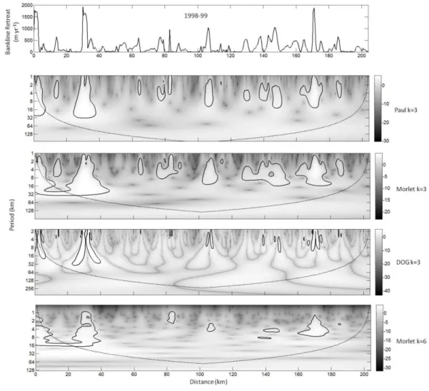
To assist in the identification of the preferred wavelet, a CWT decomposition of 376
the 1998-99 bank line retreat data was undertaken using all three wavelet functions 377
using the software developed by Torrence and Campo (1998) and implemented in 378
MATLAB. The 1998-99 data was selected because it represents one of the more complex 379
data series in the temporal sequence with a wide range of spatial scale and magnitudes 380
line retreat series implies adequate frequency localisation should be achieved with a 382
relatively low wavelet parameter (
k
) value. Moreover, the use of a small value ofk
383
reduces the area of the transform under the COI. Therefore,
k
was set to 3. However, a384
transform was also generated using a Morlet,
k
= 6 wavelet to determine the impact of385
increasing the
k
value. The results are provided in Figure 4.386
The Paul
k
=3 and Morletk
=3 wavelets can be seen to generate very similar387
patterns of significant wavelet power, associated with the same local peaks of bank line 388
retreat. There are subtle differences between the two in terms of their space / 389
frequency localisation capabilities. The Morlet
k
=3 transform exhibits some horizontal390
compression and increased lateral connectivity of the 95% confidence regions in 391
comparison with the Paul
k
=3 transform; thereby highlighting its greater frequency392
localisation capabilities. The DOG wavelet can be seen to localise peaks particularly well, 393
but at the expense of frequency. The result is lateral discontinuity in the 95% 394
confidence regions (which is also reported in De Moortel et al., 2004) and a frequency 395
localisation that is difficult to interpret. Increasing the Morlet wavelet
k
value to 6396
results in a larger COI and a loss of significant wavelet power regions at high frequencies 397
and the loss of spatial localisation (i.e. the 95% confidence regions elongate 398
horizontally); thus making it difficult to map the significant bank line retreat frequencies 399
accurately on the ground. The results indicate that both the Paul
k
= 3 and Morletk
= 3400
represent appropriate wavelet functions for the bank line retreat data series. However, 401
in this paper we use the Morlet
k
= 3 wavelet on the basis that it provides enhanced402
frequency localisation with minimal loss of spatial localisation. 403
3.3. Results 404
3.3.1. Continuous wavelet transform spectra 405
The CWT spectra for the 8 bank line retreat series (Fig. 3) calculated using an 406
of wavelet power that exceed the 95% confidence level are those within the bold lines, 408
with the dashed line indicating the COI. 409
The CWT spectra highlight two characteristic groupings of bank line retreat 410
patterns over the study period. Zones of significant wavelet power in 1996-97; 1997-98 411
and 1998-99 are largely constrained to wave periods of 16 km or less. These comprise a 412
mixture of small, very short wave periods (1-4 km) with very high spatial and frequency 413
localisation and a broader range of wave periods (2-16 km) in which the spatial and 414
frequency localisation is less well resolved. At both wave periods, significant zones are 415
spatially discrete and separated by downstream distances of between 10 and 20 km. 416
Moreover, there appears to be some temporal persistence in their location. Such 417
patterns are characteristic of locally-persistent bank line retreat events which occur 418
independently of any larger bank line retreat process (i.e. there is little evidence of local 419
bank line erosion patterns being superimposed on larger-scale, regional patterns). In 420
certain cases, the retreat is highly constrained to within a very short stretch of bank (i.e. 421
the 1-4 km wave period regions), whereas in others longer stretches are implicated (2-422
16 km period regions). 423
By contrast, zones of significant wavelet power in 1987-89; 1989-92; 1992-94 424
1994-95 and 1995-96 are characterised by the existence of longer wave periods (16-64 425
km) extending over substantial downstream distances. These are coupled, to varying 426
extents, with superimposed and locally-discrete short wave period zones, which are 427
similar in character to those of 1996-97; 1997-98 and 1998-99, but less numerous. 428
Importantly, there is some evidence of downstream movement in the locations of the 429
longer wave period significance zones, from 0 – 60 km in 1987-89; 40 – 80 km in 1992-430
94; 60 – 100 km in 1995 to 95 and 100 – 160 km in 1995-96. Such patterns are 431
difficult to interpret, yet their characteristic long wave periods, coupled with substantial 432
downstream extension and translation, would indicate that they may be characteristic of 433
bank retreat driven by the passage of a sediment-wave, or linked to the presence of 434
3.3.2. Scale averaging 436
Each of the CWTs was scale averaged into 0-10 km and 10-30 km bands 437
according to the scales of the two major downstream controls of bank retreat pattern 438
identified as operating on the Jamuna (c.f. Thorne et al., 1993). The 0-10 km band 439
encompasses the scale of individual braid-bars responsible for local bank retreat due to 440
embayment (CEGIS, 2007) and local bend evolution (Ellis, 1993). The 10-30 km band 441
encompasses the scale of island / nodal reaches associated with lower frequency 442
patterns of bank retreat governing gross-scale planform evolution (Thorne et al., 1993), 443
and the wavelength of propagating sediment waves (Takagi et al., 2007). The 444
downstream pattern of scale-averaged wavelet power exceeding the 95% confidence 445
level for each time period is plotted onto a single graph for each scale range (Fig. 6). 446
This allows the spatial and temporal persistence of different scales of bank retreat to be 447
investigated. Because the 95% confidence level of the scale-averaged wavelet power 448
varies between each time period, y-axis values are standardised as multiples of the 95% 449
confidence level for each retreat period. 450
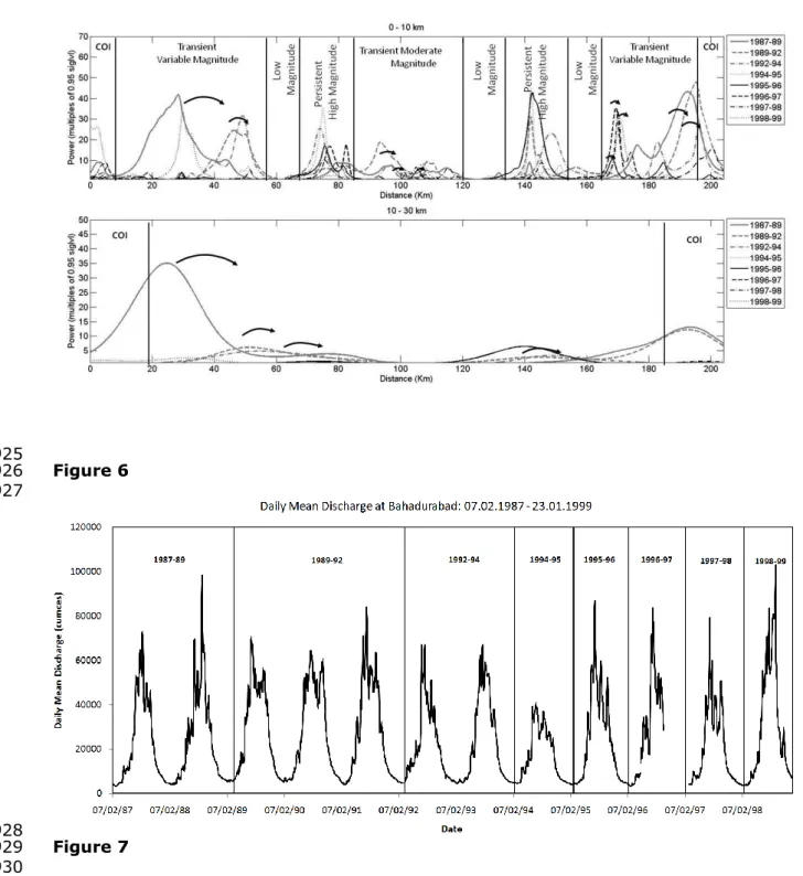
At the 0-10 km scale, the LHB can be separated into a number of clearly defined 451
reaches according to the magnitude (i.e. the wavelet power multiples above the 95% 452
confidence level) and spatio-temporal persistence (i.e. the number of consecutive years 453
wavelet power exceeds the 95% confidence level at a given location) of the bank retreat 454
patterns (Table 2). Three low-magnitude, stable reaches, which exhibit little or no 455
significant wavelet power at scales of 0-10 km, at any time period, are visible at ~57-65 456
km, ~120-135 km and ~155-164 km. The last of these is almost certainly related to the 457
existence of stable guide bunds for Jamuna Bridge (Fig. 2). In all cases, these stable 458
reaches are short; not exceeding 15 km in length. In contrast two reaches exhibit 459
persistent significant 0-10 km wavelet power throughout the majority of the study period, 460
which is, at times, of high magnitude. These are located at ~65-85 km and ~135-155 461
km. They represent reaches of moderate length (~20 km), which exhibit consistent and 462
meander bend processes. Importantly, there is little evidence of downstream translation 464
of bank line retreat with the locations of each of the main peaks in wavelet power 465
occurring within ~10 km of each other (i.e. within the bounds of the spatial localisation 466
capabilities of the Morlet
k
=3 mother wavelet). Between these two end members are a467
further three reaches in which the spatio-temporal pattern of bank retreat is transient 468
and of variable magnitude. These reaches range in length from 18 - 39 km. 469
Importantly, the transient reaches show clear evidence of downstream translation of the 470
peaks in wavelet power, as indicated by arrows in Figure 6. This may imply the 471
presence of transfer reaches where sediment eroded from the persistent, high 472
magnitude reaches is transferred downstream; instigating localised bank retreat as it is 473
transported. 474
At the island / node reach scale (10-30 km) there is little temporal persistence in 475
the locations of peak wavelet power; and thus of bank line retreat. However, the 476
existence of a stable, nodal reach at 100 - 120 km is of note. There is clear evidence of 477
downstream propagation of bank retreat. Between 1987-89 and 1995-96 a consistent 478
downstream translation of the peak wavelet power is visible, from ~25 km to ~75 km, 479
and at a mean annual rate of approximately 8 m yr-1. This pattern is consistent with 480
that of sediment wave propagation observed by Takagi et al. (2007), both in terms of its 481
scale and location. 482
The temporal analysis presented in Figure 6 provides a simplified appraisal of the 483
pattern of location and frequency variation in bank retreat through time, where the 484
complexity has been reduced through the temporal isolation of the scale-averaged power 485
spectra from each CWT. As a result, the analysis does not provide a detailed evaluation 486
of the patterns of covariance from one CWT to the next. Techniques such as cross-487
wavelet transforms and wavelet coherence analysis (Grinsted et al., 2004), that 488
specifically focus on quantifying the covariance between sequences of CWTs, offer 489
application of these advanced techniques is beyond the scope of this paper, their 491
importance as a direction for future research should be recognised. 492
3.3.3. Wavelet power relationship to discharge 493
One of the key challenges in geomorphologic studies has been establishing and 494
elucidating the relationships between processes operating over different temporal and 495
spatial scales (Rhoads and Thorn, 1996, pp. 145-6; Phillips, 1999a,b; Couper, 2004). 496
Wavelet decomposition of sequential geomorphologic signals offers potential in this 497
regard through the examination of the pattern of variability in the strength of the 498
wavelet power at different frequency localisations and time periods and its relationship 499
with potential physical drivers of the signal. 500
To this end, we also examine the relationship between different scales of bank 501
retreat and discharge by quantifying the definite integral of the downstream scale-502
averaged wavelet power spectra each time period (i.e. a numerical proxy for the total 503
magnitude of LHB retreat occurring at that scale) and plotting this against two measures 504
of peak discharge: the maximum discharge and the Q95 exceedance period (Table 3). 505
Whilst maximum discharge is identified as an important driver of bank retreat (Sarker 506
and Thorne, 2006; CEGIS, 2007), the use of variable time periods in this study means 507
that a time-integrated measure of peak discharge (i.e. Q95 exceedance) should also be 508
included in the analysis. 509
The CWT for each time period was scale-averaged into the following regular 510
intervals: 0-10 km; 10-20 km; 20-30 km; 30-40 km; 40-50 km. The definite integral of 511
each of the scale-averaged spectra for each time period was then quantified using the 512
trapezoidal rule and plotted against the peak discharge measures determined from the 513
available discharge records at the gauging station at Bahadurabad (Fig. 7). 514
At 0-10 km and 10-20 km scales, strong positive, exponential relationships are 515
seen to exist between the integral of the wave power spectrum and QMax / Q95 516
the total amount of bank retreat on the LHB of the Jamuna. It is interesting to note 518
that, in general, the strength of the relationships is stronger for maximum discharge 519
than for Q95 exceedance, suggesting that QMax may be a more useful peak discharge 520
parameter when attempting to predict bank retreat on the Jamuna. Positive 521
relationships also exist at larger scales, albeit with far lower integrated power spectrum 522
values, and lower Pearson coefficients. The positive relationships identified are not 523
unexpected as the mean rate of bank retreat on the Jamuna is known to be related to 524
the magnitude of the largest monsoon flood (Sarker and Thorne, 2006; CEGIS, 2007). 525
However, the evidence that the strength of the relationship shows a consistent decrease 526
as scale increases is new and important knowledge. Overall reductions in the magnitude 527
of the wavelet power spectrum integrals are accompanied by a reduction in R2 values as 528
scale increases. For QMax the reduction is from 0.86 at 0-10 km scales to less than 0.5 529
at scales greater than 30 km. For Q95 exceedance the reduction is from ~0.5 at scales 530
less than 20 km to ~0.3 at scales greater than 40 km. Thus, the pattern is one in which 531
peak discharge is strongly related to the rate of bank retreat on the Jamuna, but only at 532
spatial scales of less than 20 km. As the scale of bank retreat increases the importance 533
and statistical significance of peak discharge as a main driver of bank retreat is 534
substantially reduced. 535
3.4. Geomorphologic interpretation 536
A number of key characteristics of bank line retreat on the LHB of the Jamuna 537
river have been identified through the CWT analyses presented. Whilst some can be 538
interpreted with reference to well-understood geomorphologic processes and 539
conventional geomorphological thinking, others are more difficult to interpret and further 540
work is required to provide an adequate geomorphological explanation. 541
The CWT sequence in Figure 5 shows that at different times in the Jamuna river 542
data series varying amounts of significant, short (2-16 km), moderate (16-32 km) and 543
1997-98 and 1998-99), spatially-discrete regions of short wave-period bank retreat are 545
dominant and there is little evidence of significant retreat at longer periods. This 546
indicates that, at these times, the main mode of planform adjustment is local; through 547
the erosion of individual embayments. At other times (e.g. 1987-89; 1989-92; 1992-94; 548
1994-95 and 1995-96) the co-existence of significant regions of wavelet power at longer 549
wave-periods indicates that a regional mode of planform adjustment at or above the 550
scale of individual chars operates is also in operation. Indeed, in some years (1994-95 551
and 1995-96) significant regions of bank retreat at long wave-periods strongly suggest a 552
macro-scale model of adjustment that exceeds the scale of individual island chars. 553
The scale-averaged data presented in Figure 6 are more easily interpreted and 554
provide important geomorphological insights into the different characteristics of the 555
spatio-temporal patterns of bank retreat operating at different scales. At scales of 0-10 556
km the evidence of locally-persistent retreating banks, separated by stable and/or 557
transient reaches, corresponds well with the findings from other studies of local 558
embayment patterns on the Jamuna (Ellis, 1993). However, the precise reasons for the 559
alternating pattern of stable / transient / eroding reaches at this scale are not fully 560
understood. At the scales at which gross planimetric control of bank retreat by quasi-561
stable island / node reaches (10-30 km) is thought to dominate (Coleman, 1969; Thorne 562
et al., 1993) there is relatively little evidence that the locations of significant bank 563
retreat can be mapped directly to the locations of island reaches. Indeed, Thorne et al., 564
(1993) identify seven separate island and nodal reaches located at roughly regular 565
downstream spacing throughout the 204 km study reach. However, no evidence of such 566
spacing in the pattern of significant bank retreat is evident in Figure 6, and only one 567
persistently stable reach is evident. This suggests that the importance of island and 568
nodal reaches on influencing the pattern and magnitude of bank retreat at large spatial 569
scales may be less important than previously thought. Instead, the downstream 570
propagating patterns of retreat observed correspond more closely to the influence of 571
et al., 2007). Indeed, they estimated a wavelength of 35 km and found the best 573
evidence for the propagation between 10 and 80 km downstream - approximately the 574
same wavelength and location of the patterns observed in Figure 6. Thus, additional 575
support is provided to the implication that propagating sediment waves are important 576
drivers of bank retreat patterns operating at scales of tens of kilometres on the Jamuna. 577
Relating the integral of a range of scale-averaged wavelet power spectra to 578
maximum discharge and Q95 exceedance, Figures 8 and 9 provide an important and 579
explicit confirmation of conventional geomorphological thinking about the importance 580
that can be ascribed to peak discharge as a driver of bank migration at different scales 581
(e.g. Hooke, 1980; Nanson and Hickin, 1986). On the LHB of the Jamuna the magnitude 582
of the peak discharge is strongly related to the integral of the wavelet power spectrum at 583
0-10 and 10-20 km scales and, hence, the magnitude of erosion at frequencies that 584
coincide with meander bend and embayment processes. At lower frequencies, where the 585
gross planimetric setting and regional factors such as the spatial variability of floodplain 586
substrate cohesiveness become important constraints on erosion, the relationship 587
between measures of peak discharge and wavelet power decreases. 588
4. Summary and conclusions 589
The Jamuna river provides an important venue for fundamental research on 590
process-form interactions in large-scale, complex fluvial systems. It is the epitome of a 591
wilful stream representing a complex, non-linear, dynamical system within which fluvial 592
processes, morphological responses and process-response feedback loops operate at 593
multiple scales of time and space. Past efforts at understanding this system have 594
generally focussed on studying the processes governing the evolution of individual 595
geomorphological units operating at a single scale within the channel, (e.g. anabranches, 596
bars, bends and bifurcations within the braided system). Yet, their value in 597
understanding how the system operates across its whole range of scales and periods of 598
multi-scale explanatory linkage between fluvial processes and channel evolution 600
envisaged first by Schumm and Lichty (1965) and later by Lane and Richards (1997) 601
remains poorly developed. 602
CWTs offer an important means by which key signals of planimetric change, in 603
the case of this study captured as sequences of bank migration spatial series, can be 604
localised not only in time, but also in space. This offers a powerful means of 605
characterising where, when and over what spatial scales change occurs. It thus 606
represents the first, vital step in determining a multi-scale, explanatory framework for 607
relating channel process and channel pattern evolution. In many cases, it will be 608
possible to map the patterns observed to the results of past channel evolution process 609
studies. In this context, CWTs offer an important means of identifying spatio-temporal 610
patterns of bank retreat at different scales that can then be linked to fundamental 611
processes of channel adjustment and the findings of past research efforts. In other 612
cases, the patterns observed in the CWT will be more difficult to explain by conventional 613
geomorphological thinking. In these cases, CWTs offer an important means by which 614
new research directions can be identified and directed. 615
However, the outputs from a CWT are only as good as the input data. Indeed, 616
the selection of a planimetric signal capable of providing an adequate characterisation of 617
the evolutionary processes of interest is critical. For example, whilst sequences of bank 618
line retreat series offer important insights into erosion processes, they provide no 619
information about the temporal, spatial and frequency scales at which deposition occurs. 620
This means that an important component of channel change processes are 621
uncharacterised and the links between depositional and erosional channel forms can only 622
be surmised; not explicitly demonstrated. Similarly, by focussing on a single bank line, 623
only half of the channel's erosion response is characterised. Consequently, determining 624
the optimum set of channel response signals to which CWT should be applied in order to 625
gain a more holistic characterisation of the patterns of channel evolution is a pressing 626
used. Where the length of the data series is short, the relatively large size of the COI 628
will limit the ability to localise low frequency responses in the data. The downstream 629
resolution of the data will ultimately determine the degree to which high frequency 630
responses can be localised. Similarly, the length of time over which the signal is 631
measured, relative to the return period of the fluvial processes responsible for those 632
changes, may reduce the magnitude of certain responses when the data are converted 633
to annual rates. This in turn will reduce their wavelet power in the CWT and may result 634
in their significance being underestimated. 635
To conclude, the results presented in the paper represent an early, exploratory 636
investigation of the usefulness of wavelet transformation of signals of planimetric change 637
in complex river systems. Considerable potential for the technique is evident, however 638
numerous questions remain and both wavelet analysis in general and CWT in particular 639
offer considerable opportunities for fruitful future research efforts in unravelling river 640
pattern change. 641
Acknowledgements 642
Wavelet software was provided by C. Torrence and G. Compo, and is available at 643
URL: http://atoc.colorado.edu/research/wavelets/. NJM and NJT thank the Universities 644
of Nottingham and Leicester for the granting of research study leave coinciding with this 645
research. 646
647
648
649
650
651
References 653
Ashworth, P.J., Best, J.L., Roden, J.E., Bristow, C.S., Klaassen, G.J., 2000. 654
Morphological evolution and dynamics of a large, sand-braid bar, Jamuna River, 655
Bangladesh. Sedimentology 47, 533-555. 656
Best, J.L., Bristow, C.S. 1993., Braided rivers: perspectives and problems. In: Best, 657
J.L.,Bristow,C.S. (Eds.), Braided Rivers. Geological Society of London Special Publication 658
75, Geological Society, London. pp. 1–11. 659
Biswas, A., Si, B.C., 2011. Application of continuous wavelet transform in examining soil 660
spatial variation: A review. Mathematical Geosciences 43, 379–396. 661
Brillinger, D.R. 1994., Trend analysis: time series and point process problems. 662
Environmetrics 5, 1-19. 663
Burger, J., Klaassen, G.J., Prins, A. 1991., Bank erosion and channel processes in the 664
Jamuna River. In: Elahi, K.M., Ahemd, K.S., Mofizuddin, M. (Eds.), Riverbank Erosion, 665
Flood and Population Displacement in Bangladesh. Riverbank Impact Study, 666
Jahangirnagar University, Dhaka, Bangladesh. 667
Camporeale, C., Perona, P., Porporato, A., Ridolfi, L., 2005. On the long-term behavior 668
of meandering rivers. Water Resources Research 41, W12403. 669
Centre for Environmental and Geographical Information Services (CEGIS), 1997. 670
Morphological Dynamics of the Jamuna River. Water Resources Planning Organization, 671
Ministry of Water Resources, Government of the People's Republic of Bangladesh, Dhaka. 672
76pp. 673
CEGIS, 2000. Riverine Chars in Bangladesh: Environmental Dynamics and Management 674
CEGIS, 2001. Remote Sensing, GIS and Morphological Analyses of the Jamuna River. 676
Part II. River Bank Protection Project, Bangladesh Water Development Board, Dhaka, 677
Bangladesh. 678
CEGIS, 2007. Long-term erosion process of the Jamuna river. Centre for Environmental 679
and Geographic Information Services, Dhaka, 74 pp. 680
Coleman, J.M., 1969. Brahmaputra River. Channel processes and sedimentation. 681
Sedimentary Geology 8, 129-239. 682
Compagnucci, R.H., Blanco, S.A., Filiola, M.A., Jacovkis, P.M., 2000. Variability in 683
subtropical Andean Argentinian Atuel river: a wavelet approach. Environmetrics 11, 684
251-269. 685
Coulibaly, P., Burn, D.H., 2004. Wavelet analysis of variability in annual Canadian 686
streamflows. Water Resources Research 40, W03105. 687
Couper, P.R., 2004. Space and time in river bank erosion research: a review. Area 36, 688
387-403. 689
De Moortel, I., Munday, S., Hood, A. W., 2004. Wavelet analysis: the effect of varying 690
basic wavelet parameters. Solar Physics 222, 203-228. 691
Daubechies, I., 1992. Ten Lectures on Wavelets. Society for Industrial and Applied 692
Mathematics, Philadelphia. 357 pp. 693
Downward, S.R., Gurnell, A.M., Brookes, A., 1994. A methodology for quantifying river 694
channel change using GIS. In: Olive, L.J., Loughran, R.J., Kesby, J.A. (Eds.), Variability 695
in Stream Erosion and Sediment Transport, Proceedings of the Canberra Symposium 696
1994, IAHS Publication No. 224, IAHS Press, Wallingford, pp. 449-456. 697
Ellis, L., 1993. River Bank Erosion and Different Hydrologic Regimes. Unpublished MPhil 698
Flood Action Plan-1 (FAP-1), 1991. River Training Studies of the Brahmaputra River, 700
second interim report. Sir William Halcrow and Partners Ltd., London. 701
FAP-1, 1992. River Training Studies of the Brahmaputra River, draft final report. Sir 702
William Halcrow and Partners Ltd., London. 703
Farge, M., 1992. Wavelet transforms and their application to turbulence. Annual Review 704
of Fluid Mechanics 24, 395-457. 705
Ferguson, R.I., 1975. Meander irregularity and wavelength estimation. Journal of 706
Hydrology 26, 315-333. 707
Ferguson, R.I., 1993. Understanding braiding processes in gravel-bed rivers: progress 708
and unsolved problems. In: Best, J.L., Bristow, C.S. (Eds.), Braided Rivers. Geological 709
Society Special Publication 75, Geological Society, London, pp. 73-87. 710
Fournier, A., 1995. Wavelets and their applications in computer graphics, SIGGRAPH'95 711
Course Notes, pp. 5–35. 712
Fougere, P.F., 1985. On the accuracy of spectrum analysis of red noise processes using 713
maximum entropy and periodogram methods: simulation studies and application to 714
geophysical data. Journal of Geophysical Research 90(A5), 4355-4366. 715
Fraedrich, K., Jiang, J., Gerstengarbe, F-W., Werner, P.C., 1997. Multiscale detection of 716
abrupt climate changes: application to the river Nile flood. International Journal of 717
Climatology 17, 1301-1315. 718
Fu, S., Muralikrishnan, B., Raja, J., 2003. Engineering surface analysis with different 719
wavelet bases. Journal of Manufacturing Science and Engineering 125, 844-852. 720
Gaucherel, C., 2002. Use of wavelet transform for temporal characterisation of remote 721
watersheds. Journal of Hydrology 269, 101-121. 722
Gilbert, G.K., 1917. Hydraulic mining debris in the Sierra Nevada. US Geological Survey 723
Goswami, D.C., 1995. Brahmaputra River, Assam, India: physiography, basin 725
denudation and channel aggradation. Water Resources Research 21, 959-978. 726
Goswami, U., Sarma, J.N., Patgiri, A.D., 1999. River channel changes of the Subansiri in 727
Assam, India. Geomorphology 30, 227-244. 728
Graps, A., 1995. An introduction to wavelets. IEEE Computational Science and 729
Engineering 2, 50-61. 730
Grinsted, A., Moore, J.C., Jevrejeva, S., 2004. Application of the cross wavelet 731
transform and wavelet coherence to geophysical time series. Nonlinear Processes in 732
Geophysics 11, 561-566. 733
Gurley, K., Kareem, A., 1999. Applications of wavelet transforms in earthquake, wind, 734
and ocean engineering. Engineering Structures 21, 149-167. 735
Gurnell, A.M., 1997. Channel change on the River Dee meanders, 1946-1992, from the 736
analysis of air photographs. Regulated Rivers Research and Management 13, 13-26. 737
Gurnell, A.M., Downward, S.R., Jones, R., 1994. Channel planform change on the River 738
Dee meanders, 1876-1992. Regulated Rivers Research and Management 7, 247-260. 739
Halcrow, Sir William and Partners, DHI, EPC and DIG, 1994. River Training Studies of the 740
Brahmaputra River, Final Report, Annex 2: Morphology. Bangladesh Water Development 741
Board (BWDB), Dhaka, Bangladesh. 88 pp. 742
Hooke, J., 1980. Magnitude and distribution of rates of river bank erosion. Earth 743
Surface Processes and Landforms 5, 143-157. 744
Ikeda, S., Parker, G., Sawai, K., 1981. Bend theory of river meanders. part 1. linear 745
development. Journal of Fluid Mechanics 112, 363-377. 746
ISPAN, 1995. The Dynamic Physical Environment of Riverine Charlands: Jamuna, 747
Irrigation Support Project for Asia and near East (ISPAN), Flood Plan Coordination 748
Johannesson, H., Parker, G., 1989. Linear theory of river meanders. In: Ikeda, H., 750
Parker, G. (Eds.), River Meandering. Water Resources Monographs 12, American 751
Geophysical Union, Washington, DC. pp. 181-214. 752
Khan, N.I., Islam, A., 2003. Quantification of erosion processes in the Jamuna River 753
using geographical information systems and remote sensing techniques. Hydrological 754
Processes 17, 959-966. 755
Kleinhans, M.G., 2010. Sorting out river channel patterns. Progress in Physical 756
Geography 34, 287-326. 757
Kumar, P., Foufoula-Georgiou, E., 1997. Wavelet analysis for geophysical applications. 758
Reviews of Geophysics 35, 385-412. 759
Labat, D., 2005. Recent advances in wavelet analyses: Part 1. A review of concepts. 760
Journal of Hydrology 314, 275-288. 761
Labat, D., Ababou, R., Mangin, A., 1999. Wavelet analysis in karstic hydrology: part 1. 762
Comptes Rendues de l’Academie des Sciences: Geosciences de Surface 329, 881–887. 763
Labat, D., Ababou, R., Mangin, A., 2000. Rainfall-runoff relations for karstic springs. 764
Part II: continuous wavelet and discrete orthogonal multiresolution analyses. Journal of 765
Hydrology 238, 149-178. 766
Labat, D., Ababou, R., Mangin, A., 2002. Analyse multiresolution croisee de pluies et 767
debits de sources karstiques. Comptes Rendues de l’Academie des Sciences: 768
Geosciences de Surface 334, 551–556. 769
Lafreniere, M., Sharp, M., 2003. Wavelet analysis of inter-annual variability in the runoff 770
regimes of glacial and nival stream catchments, Bow Lake, Alberta. Hydrological 771
Processes 17, 1093-1118. 772
Lane, S.N., 2007. Assessment of rainfall-runoff models based upon wavelet analysis. 773
Lane, S.N., Richards, K.S., 1997. Linking river channel form and process: Time space 775
and causality revisited. Earth Surface Processes and Landforms 22, 249-260. 776
Latrubesse, E.M., 2008. Patterns of anabranching channels: the ultimate end-member 777
adjustment of mega rivers. Geomorphology 101, 130-145. 778
Madej, M.A., Ozaki, V., 1996. Channel response to sediment wave propagation and 779
movement, Redwood Creek, California, USE. Earth Surface Processes and Landforms 21, 780
911-927. 781
Marcus, W.A., Fonstad, M.A., 2010. Remote sensing of rivers: the emergence of a 782
subdiscipline in the river sciences. Earth Surface Processes and Landforms 35, 1867-783
1872. 784
Milne, A.E., Webster R., Lark, R.M., 2010. Spectral and wavelet analysis of Gilgai 785
patterns from air photography. Soil Research 48, 309–325. 786
Mount, N.J., Louis, J., 2005. Estimation and propagation of error in measurements of 787
river channel movement from aerial imagery. Earth Surface Processes and Landforms 788
30, 635-643. 789
Mount, N.J., Louis, J., Teeuw, R.M., Zukowski, P.M., 2003. Estimation of error in 790
bankfull width comparisons from temporally sequenced raw and corrected aerial 791
photographs. Geomorphology 56, 65-77. 792
Nanson, G. C., Hickin, E.J., 1986. A statistical analysis of bank erosion and channel 793
migration in western Canada. Geological Society of America Bulletin 97, 497-504. 794
Nason, G.P., 2008. Wavelet Methods in Statistics with R. Springer, New York. 260 pp. 795
Parker, G., Diplas, P., Akiyama, J., 1983. Meander bends of high amplitude. Journal of 796
the Hydraulics Division ASCE 109, 1323-1337. 797
Percival, D.B., Wang, M., Overland, J.E., 2004. An introduction to wavelet analysis with 798
Phillips, J.D., 1999a. Earth Surface Systems: Complexity, Order and Scale. Blackwell, 800
Oxford, 180 pp. 801
Phillips, J.D., 1999b. Methodology, scale and the field of dreams. Annals of the 802
Association of American Geographers 89, 754-760. 803
Richardson, W.R., 1997. Secondary Flow and Channel Change in Braided Rivers. 804
Unpublished PhD Thesis, School of Geography, University of Nottingham, UK, 281 pp. 805
Richardson, W.R., Thorne, C.R., 2001. Multiple thread flow and channel bifurcation in a 806
braided river: Brahmaputra–Jamuna River, Bangladesh. Geomorphology 38, 185–196. 807
Rhoads, B.L., Thorn, C.R., 1996. The Scientific Nature of Geomorphology. Wiley, 808
Chichester, 481 pp. 809
Sadowsky, J., 1996. Investigation of signal characteristics using the continuous wavelet 810
transform. Johns Hopkins APL Technical Digest 17, 258-269. 811
Sankhua, R.N., Sharma, N., Garg, P.K., Pandey, A.D., 2005. Use of Remote Sensing and 812
ANN in assessment of erosion activities in Majuli, the world's largest river island. 813
International Journal of Remotes Sensing 26, 4445-4454. 814
Sarma, J.N., 2005. Fluvial processes and morphology of the Brahmaputra River in 815
Assam, India. Geomorphology 70, 226-256. 816
Sarma, J.N., Basumallick, S., 1984. Bankline migration of the Burhi Dihing river, Assam. 817
Indian Journal of Earth Sciences 11, 199-206. 818
Sarma, J.N., Phukan, M.K., 2004. Origin and some geomorphological changes of Majuli 819
Island of the Brahmaputra River in Assam, India. Geomorphology 60, 1-19. 820
Sarma, J.N., Phukan, M.K., 2006. Bank erosion and bank line migration of the 821
Brahmaputra river in Assam during the twentieth century. Journal of the Geological 822
Sarker, M.H., Thorne, C.J., 2006. Morphological response of the Brahmaputra-Padma-824
Lower Meghna river system to the Assam earthquake of 1950. In: Sambrook Smith, G. 825
H., Best, J. L., Bristow, C.S., Petts, G. E. (Eds.), Braided Rivers: Process, Deposits, 826
Ecology and Management. IAS Special Publication, 36, Blackwell Publishing, Oxford, pp. 827
289-310. 828
Schumm, S.A., Lichty, E.W., 1965. Time, space and causality in geomorphology. 829
American Journal of Science 263, 110-119. 830
Si, B.C., Farrell, R.E., 2004. Scale dependent relationships between wheat yield and 831
topographic indices: A wavelet approach. Soil Science of America Journal 68, 577–588. 832
Singh, I.B., Bajpai, V.N., Kumar, A., Singh, M., 1990. Changes in the channel 833
characteristics of Ganga River during late Pleistocene-Holocene. Journal of the 834
Geological Society of India 36, 67-73. 835
Swanson, B.J., Meyer, G.A., Coonrod, J.E., 2011. Historical channel narrowing along the 836
Rio Grande near Albuquerque, New Mexico in response to peak discharge reductions and 837
engineering: magnitude and uncertainty of change from air photo measurements. Earth 838
Surface Processes and Landforms 36, 885-900. 839
Takagi, T., Oguchi, T., Matsumoto, J., Grossman, M.J., Sarher, M.H., Matin, M.A., 2007. 840
Channel braiding and stability of the Brahmaputra River, Bangladesh, since 1967: GIS 841
and remote sensing analyses. Geomorphology 85, 294-305. 842
Thorne, C.R., Russell, P.G., 1993. Geomorphic study of bankline movement of the 843
Brahmaputra River, Bangladesh. Proc. 5th Annual Seminar of the Scottish Hydraulics 844
Study Group on Sediment Transport Processes and Phenomena. Edinburgh, UK. 845
Thorne, C.R., Russell, P.G., Alam, M.K., 1993. Planform pattern and channel evolution of 846
the Brahmaputra River, Bangladesh. In: Best, J.L., Bristow, C.S. (Eds.), Braided Rivers. 847
Geological Society of London Special Publication 75, Geological Society, London, pp. 257-848