Face Recognition and Verification using
Photometric Stereo: The Photoface Database
and a Comprehensive Evaluation
Stefanos Zafeiriou, Gary A. Atkinson, Mark F. Hansen, William A. P. Smith, Vasileios
Argyriou, Maria Petrou, Melvin L. Smith and Lyndon N. Smith
Abstract
This paper presents a new database suitable for both 2D and 3D face recognition based on photometric
stereo (PS): the Photoface database. The database was collected using a custom-made four-source PS device designed to enable data capture with minimal interaction necessary from the subjects. The device,
which automatically detects the presence of a subject using ultrasound, was placed at the entrance to
a busy workplace and captured 1839 sessions of face images with natural pose and expression. This
meant that the acquired data is more realistic for everyday use than existing databases and is, therefore,
an invaluable test bed for state-of-the-art recognition algorithms. The paper also presents experiments
of various face recognition and verification algorithms using the albedo, surface normals and recovered
depth maps. Finally, we have conducted experiments in order to demonstrate how different methods in
the pipeline of PS (i.e. normal field computation and depth map reconstruction) affect recognition and
verification performance. These experiments help to (1) demonstrate the usefulness of PS, and our device
in particular, for minimal-interaction face recognition, and (2) highlight the optimal reconstruction and
recognition algorithms for use with natural-expression PS data.
Index Terms
S. Zafeiriou is with the Department of Computing, Imperial College London, United Kingdom. Email:
Gary Atkinson, Mark F. Hansen, Melviun L. Smith and Lyndon N. Smith are with Machine Vision Lab, Faculty of
Environment and Technology, University of the West of England, Frenchay Campus, Bristol BS16 1QY UK, Emails: {gary.atkinson,mark.hansen,melvyn.smith,lyndon.smith}@uwe.ac.uk
Vasileios Argyriou is with the Faculty of Computing, Information Systems and Mathematics, Kingston University London,
River House, 53-57 High Street, Kingston upon Thames, Surrey KT1 1LQ UK. Email: [email protected] William A. P. Smith is with Department of Computer Science University of York, UK. Email: [email protected]
Maria Petrou is with Informatics and Telematics Institute, Centre of Research & Technology - Hellas 6th km Xarilaou - Thermi, Thessaloniki 57001 Greece and also with Department of Electrical and Electronic Engineering, Imperial College London, Exhibition Road, South Kensington Campus, London SW7 2AZ UK, Email: [email protected]
photometric stereo, face recognition/verification, face database
I. INTRODUCTION
There have been a plethora of face recognition algorithms published in the literature during the last
few decades. During this time, a great many databases of face images, and later 3D scans, have been
collected as a means to test these algorithms. Each algorithm has its owns strengths and limitations and
each database is designed to test a specific aspect of recognition. This paper is motivated by the desire
to have a face recognition system operational where users do not need to interact with the data capture
device and do not need to present a particular pose or expression. While we do not completely solve
these immensely challenging problems in this paper, our aim is to contribute towards this endeavour by
means of:
1) Construction of a novel 3D face capture system, which automatically detects subjects casually
passing the device and captures their facial geometry using photometric stereo (PS) – a 3D
reconstruction method that uses multiple images with different light source directions to estimate
shape [2]. To the best of our knowledge this is one of the first realistic commercial acquisition
arrangement for the collection of 2D/3D facial samples using PS.
2) Collection of a 2D and 3D face database using this device, with natural expressions and poses.
3) Detailed experiments on a range of 3D reconstruction and recognition/verification algorithms to
demonstrate the suitability of our hardware to the problem of non-interactive face recognition. The
experiments also show which reconstruction and recognition methods are best for use with natural
pose/expression data from PS. This is one of the first detailed experimental studies to demonstrate
how different methods in the pipeline of PS affect recognition/verification performance.
II. RELATED WORK AND CONTEXT
A. Face databases
Face recognition researchers have been collecting databases of face images for several decades now
[3, Chapter 13]. While some databases can be regarded as superior to others, each of them are designed
to test different aspects of recognition and have their own strengths and weaknesses. One of the largest
databases available is the FERET database [4]. This has a total of 1199 subjects with up to 20 poses,
two expressions and two light source directions. The FERET database was originally acquired using a
35mm camera. Others, for example the widely used CMU PIE database [5] or the Harvard RL database
[6], concentrate specifically on varying the capture conditions such as pose and illumination. Another
popular database collected for the purpose of face verification under well-controlled conditions is the
XM2VTS database [7].
The PIE database is one of the most extensively researched. This is due to the fact that the faces
B database [8] offers similar advantages to the PIE databases except with an even larger number of
lighting conditions (64) using nine poses. However, the Yale B database includes just ten subjects. The
original Yale database [9] was designed to consider facial expressions, with six types being imaged for 15
subjects. Finally, the extended Yale B database was published which contains 28 subjects with 9 different
poses and 64 illumination conditions [10].
Even though the PIE [5], Yale [8] and extended Yale [10] databases provide facial samples taken under
different illumination directions they contain few subjects. More recently, the CMU Multi-PIE database
[11] has been constructed with the aim of extending the image sets to include a larger number of subjects
(337) and to capture faces taken in four different recording sessions. This database was recorded under
controlled laboratory conditions, as with the others mentioned above.
A recently emerged trend in face recognition research has been to incorporate three-dimensional
information into the recognition process. This has naturally lead to the collection of databases with 3D
facial samples1. This trend is due to the fact that changes in viewing conditions (e.g. lighting variation) adversely affect the 2D appearance of a face image but not the 3D appearance. The number of existing
databases containing 3D facial samples suitable for 3D face recognition is constantly increasing. In the
what follows we briefly present the publicly available ones, categorizing them according to the degree
of difficulty in obtaining 3D face samples and their equipment cost.
1) 3D Face databases: One of the first publicly available datasets containing 3D face samples for face verification was presented in [13], [14]. The database contains approximately 100 subjects. It was
collected using the structured light technology, a low cost technology that is widely used in our days
(for example in kinect). However, despite the obvious advantage of being of low cost, the commodity
structured light technologies offer smaller spatial resolution, resulting in that way in samples that appear
to have missing parts and holes. More recent publicly available databases that employ more sophisticated
commercial structured light technology include the Bosphorus [15] and the University of York 3D [16],
[17] databases. The Bosphorus database, that can be used both for facial expression and face recognition
experiments, was captured using a commercial structured light based 3D digitizer device, the Inspeck
Mega Capturor II 3D 2. It contains (the face recognition experiments version) 47 subjects with 53 face scans per subject. The University of York 3D face database consists of 350 subjects with different facial
expressions (happiness and anger) as well as images with closed eyes and raised eyebrows.
One of the most widely known datasets of 3D facial samples is the FRGC database [18] and its
extension, namely ND 2006 [19]. The FRGC database is a multi-partition 2D and 3D database that
contains a validation set consisting of 466 subjects to a total of 4007 images. The ND-2006 database was
1
Another trend in face recognition is totally unconstrained face matching (suitable for face tagging experiments) and a database for this task called “Labelled Faces in the Wild” has been recently collected [12], but this trend is out of the scope of the paper,
since in this paper we aim at describing a database suitable for an industrial setting.
2
captured using a rather expensive camera, the Minolta Vivid 910 laser range scanner [20], that provided
3D face samples of up to 112,000 vertices. The database consists of 888 subjects and multiple images per
subject of various posed facial expressions (happiness, disgust, sadness and surprise). Another database
that was collected using the same camera is the CASIA 3D Face database [21], [22]. It consists of 123
subjects with 10 images per subject displaying different facial expressions (smile, laughter, anger and
surprise) and closed eyes.
A laser digitizer (the Minolta VI-700 digitizer) was used for capturing the GavabDB database [23]. It
contains 61 subjects (all Caucasian) displaying different smiles (open/closed mouth) and random facial
expressions that each subject chose. Two publicly available databases that have been mainly used for
3D/4D facial expression recognition but could also be used for face recognition, are the BU3D [24] and
BU4D [25] databases. Both of the databases were captured using 3DMD acquisition setups, combining in
that way passive and active stereo. However, these setups are of high cost and require the full collaboration
of the subject. Both of the databases consist of approximately 100 images, but unfortunately they contain
only one session, something that does not meet with the requirements for face recognition. The Texas 3D
Face Recognition Database [26], [27] consists of 3D models that were captured using an MU-2 stereo
imaging system (similar to the used in BU3D) and contains 105 subjects.
The purpose of the new database described in this paper is to capture a large number of faces in
3D from a more industrial setting. However, most existing 3D capture devices (e.g. [28], [20]) are both
financially and computationally expensive which can be highly inhibiting for commercial application. By
contrast, we use a four-source high-speed capture arrangement (which now can be easily deployed with
even less than 2K ), which permits the use of PS methods [2] to recover the 3D information with minimal
computational expense. Furthermore the device is significantly financially cheaper than most other 3D
capture mechanisms. A photograph of our device is shown in Fig. 1 and will be explained in more detail
in Section III.
Another advantage of our capture mechanism is that PS methods have a one-to-one relationship between
the surface normals and the resolution of the acquired image. This means that each pixel corresponds to
a facet with one normal. Moreover, methods that provide subpixel reconstructions using PS are available
[29] allowing lower resolution capturing devices to provide detailed estimates. It should be mentioned
that this one-to-one relationship allows detailed reconstructions with applications in other areas such as
object inspection for defects, surveillance and recognition.
So the aim here is to capture poses and expressions that are as natural as possible. For this reason, we
placed our capture device near the entrance to a busy workplace and gave all of the volunteer subjects
the sole instruction to “walk through the archway”. The database therefore offers an ideal testbed for
face recognition algorithms designed for real world applications where minimal interaction is desired.
As PS can be applied to the four images (one image per light source) to calculate the 3D structure of
Fig. 1. The image capture device. One of the light sources and an ultrasound trigger are shown to the left. The camera is located at the back panel.
consists of 1,839 capture sessions of 261 subjects.
B. Reconstruction and Recognition methods for PS data
In addition to describing the device and the database, we also present experiments on the Photoface
database by applying face recognition and verification techniques on the albedo, depth and surface normal
images – all of which may be calculated from PS. For the case of the albedo, we applied algorithms
from two of the most popular families of face recognition from intensity images:
1) subspace methods such as Principal Component Analysis (PCA), Nonnegative Matrix Factorization
(NMF), Linear Discriminant Analysis (LDA) [30], [31] etc using the vectorized albedo images as
feature vectors,
2) feature-based methods using Elastic Graph Matching (EGM) architectures [32], [33], [34].
For the depth map, we applied exactly the same methods as in the case of albedo images. Finally, for the
normals we propose a novel method based on metric-multidimensional scaling of theL1-norm of angles.
We stress at this point that the experiments are intended to test the various algorithms on PS data of
natural pose and expression specifically. The focus therefore is neither to compare various 2D/3D face
recognition and verification methods against each other for general application nor to demonstrate that
fusion of information of 3D and 2D data increase the recognition performance [35],[36]. A comparative
study of 3D face recognition/verification methods was recently published in [36], where a large inventory
of 3D recognition methods were implemented and tested on various representations of facial geometry
(i.e. depth images and normal fields). Moreover, the authors of [36] applied various fusion strategies on
the results of 3D face recognition methods. Another recent study on the fusion of information of intensity
The aims of the experiments conducted in this paper are:
• to demonstrate how different methods in the pipeline of PS (i.e. normal field computation and depth map reconstruction methods) affect recognition/verification performance
• to verify that a similar conclusion to [35] can be drawn for the modalities derived from PS methods. In particular we would like to verify that (1) similar recognition performance can obtained using
a single 2D intensity image or a single 3D image (or normal field), (2) 2D+3D face recognition
performs better than using either 3D or 2D alone and (3) fussing results from two 2D or 3D images
using a similar fusion scheme as used in multimodal 2D+3D also improves performance over using
a single 2D image.
We applied three different PS methods in order to compute the normal field and the albedo image and
five different integration methods that compute the height map from the normal field. To the best of the
authors’ knowledge this is the first experiment on a real-world PS database which also explores the affect
of the use of different methods in the processing pipeline.
The rest of the paper is organised as follows. In Section III the device for image capture and the
collected database is described. In Section IV, we describe the PS methods for the computation of the
albedo and normal field. In Section V we describe the methods for surface reconstruction. In Section
VI we describe the methods we tested for face recognition using albedo, depth maps and normal fields.
Experimental results are described in Section VII. Finally, conclusions are drawn in Section VIII.
III. HARDWARE AND DATABASE COLLECTION
A. The Device
The Photoface database was collected using the custom-made four-source PS device shown in Fig. 1.
Unlike previous constructions, our aim was to capture the data using hardware that could easily be
deployed in commercial settings. Individuals are told to walk through the archway towards the camera
located on the back panel and exit through the side. This arrangement makes the device suitable for usage
at entrances to buildings, high security areas, airports etc. The presence of an individual is detected by
an ultrasound proximity sensor placed before the archway. This can be seen in Fig. 1 on the horizontal
beam towards the left-hand side of the rig.
The hardware components used to create the system were as follows:
• Camera: Basler 504kc with Camera Link interface operating at 200fps. 1ms exposure time. Placed at a distance of approximately 2m from the head of the subject.
• Lens: 55mm, f5.6 Sigma lens.
• Light sources: low cost Jessops M100 flashguns, at a distance of approximately 75cm from the head of the subject.
• Hardware IO card (for interfacing the camera, frame grabber and light sources): NI PCI-7811 DIO with Field Programmable Gate Array (FPGA).
• Frame grabber: NI PCIe-1429.
• Interfacing code: NI LabVIEW (the reconstruction and recognition algorithms were written in MATLAB).
The device also contains a monitor (as can be seen in Fig. 1) that provides instructions and could be
used to indicate whether or not an individual was recognised in the case of a recognition scenario, or
whether an identity claim was accepted or rejected in the case of a verification scenario.
The device captures one image of the face for each light source in a total of approximately 20ms. This
rate of image capture, which we adopt for all our experiments, was regarded as adequate to reduce the
inter-frame motion to below a few pixels. The only case in which the performance of the system can be
expected to deteriorate significantly, is when a person runs through the device. This required frame rate
was determined through experimentation. Fig. 2 shows an example of four raw images of an individual.
The resolution of the original image captured is1280×1024px, although the images in our database are
automatically [37] cropped to the face itself (typically of the order 600×800px).
The capture device was placed at the entrance of a busy workplace for a period of four months.
Volunteer employees casually passed through the booth at regular intervals throughout this period. No
instructions were given, other than to ask them to walk through the archway towards at the camera and
monitor. Thus, the volunteers typically passed through the device on their way in and out of the building.
This arrangement is of great importance for face recognition testing as:
1) It meant that the capture conditions were realistic for a real-world example. This is in contrast with
existing face databases such as the widely used CMU-PIE database [11] or the FRGC database
[18].
2) The whole set-up was non-invasive, thus being suitable for any recognition algorithms developed
for immediate commercial use.
B. Statistics of the Database
The Photoface database was collected between February and June 2008. It consists of a total of 1,839
sessions of 261 subjects and a total of 7,356 images. Some individuals used the device only once,
while others walked through it more than 20 times. The majority of people in the database are male
(227 compared to 34 female). Furthermore, the subjects are predominantly Caucasian (257 subjects).
Due to the lack of supervision, most of the captured faces in the database display an expression (for
example, more than 600 smiles and more than 200 surprises, open mouth, scream like expression etc.
were recorded).
Regarding repeat usages, 98 people walked through the device only once. For 126 of the 163 subjects
interval. For the majority of those (90 people), this interval was greater than one month. The number of
images corresponding to the number of subject recordings by the device is depicted in Fig. 3.
IV. PHOTOMETRICSTEREO FORSURFACENORMALCOMPUTATION
This section presents the various PS methods that we adopt to estimate the surface normal at each
pixel from the raw images. We first summarise the original method [2],[38, Section 5.4], which we later
apply to three and four sources. This is followed by a ray tracing method and an optimisation method:
both of which aim to diminish complications such as shadows and highlights.
A. Standard Photometric Stereo
The original method for PS assumes Lambert’s Law and essentially derives a matrix equation for the
expected intensity at each pixel for given light source directions, l, and surface albedo, ρ. For a single
light source, Lambert’s law can be written for a pixel at location x= [x, y]T as
I(x) =ρ(x)lTn(x) (1)
where I(x) is the measured pixel intensity andn(x)is the surface normal. This is extended toN light
sources using the following matrix equation:
[I1(x) I2(x)· · ·IN(x)]T =ρ(x)
[
lT1 lT2 · · ·lTN]T n(x) (2) where Im(x) is themth measured pixel intensity andlm is the mth light source vector. Using measured
intensity values from the images and assuming that the light source vectors are known a-priori, we can
then use this equation to solve for the albedo and the surface normal components at each pixel. Note the
assumption that the camera response is linear.
We have mainly concentrated on a four-source version of the technique, although we have also
compared our results to methods using three sources. For the latter, we omitted the upper-right source in
Fig. 1 from the computation. The choice of which source to remove was somewhat arbitrary although
we should note that the choice does have an impact on the reconstructions as some sources cause more
shadows than others.
B. A Ray Tracing Method for Photometric Stereo
In many cases of PS usage, it is desirable to use all available light sources in the reconstruction in order
to maximise robustness. However, where one or more sources do not illuminate the entire surface due to
a self/cast shadow, it becomes disadvantageous to use all the sources. In the case of a face, this is most
likely to happen around the nose and outer edges of the cheeks, as shown in Fig. 2. Argyriou and Petrou
recently proposed a recursive algorithm for PS in the presence of self and cast shadows and highlights
Initially, the problematic areas of the surface are identified based on the fact that there exists be a
linear equation expressing the relationship between theN illumination direction vectors. In the next step,
standard PS is applied, and prior to integration, the problematic areas are removed. The self and the cast
shadows are then estimated from the reconstructed surface from ray tracing. Using the newly available
information on shadows, PS is applied again using only the useful (i.e, those not causing shadow or
highlights) lights. If erroneous areas still exist, they are regarded as highlights and the corresponding
illumination sources are removed. In the final step, PS is applied using the shadow and highlight free
sources.
This reconstruction method is therefore able to identify areas where some of the lighting directions
result in unreliable data, providing the capability to adjust a reconstruction algorithm and improve its
performance accordingly. The main advantage is that it does not rely on individual pixels to locate
shadows, but is based on the entire surface resulting in more reliable shadow maps.
C. Mitigation of shadow effects
Another recently proposed method to address shadow effects was presented by Hansen et al. [40]. This
method assumes that no points on the face are shadowed by more than one source. The surface normal
that is adopted for each point is then taken as a linear combination of the estimate using all four sources
and that using the best combination of three sources.
More formally, the optimal surface normal estimate nopt is given by:
nopt(x, ε(x)) =ε(x)n3(x) + (1−ε(x))n(x) (3)
whereεis a measure of the likelihood of a pixel being in shadow andn3 is the surface normal estimated
from the optimal three light sources. The value ofε varies between 0 and 1. For the case where ε= 0,
the pixel in question is definitely not in shadow and so all four sources are used. Forε= 1, the pixel is
deep in shadow, so only three sources are used. For intermediate values ofε, a mixture ofn andn3 are
used.
The vector n3 is calculated using (2) with N = 3 and the three light sources are chosen that give the
brightest intensities. The mixing factor,ε, is determined based on the discrepancy between the measured
intensity corresponding to the light source not used to calculate n3 and the expected value based on
Lambert’s Law and n3.
V. FROMSURFACENORMALS TOSURFACES
In this section we review the problem of reconstructing a surface (often called a depth map) from the recovered field of surface normals. This suggests representing the surface as (x, f(x))
n(x) = √ 1
1 +∂f∂x2+∂f∂y2
( −∂f
∂x,− ∂f ∂y,1
)T
Let us assume that the computed value of the unit normal at some point xisn(x) = [a(x), b(x), c(x)]T,
as calculated by (2) for example. Then
∂f ∂x = a(x) c(x) ∂f ∂y = b(x)
c(x). (5)
To recover the depth map, we need to determine f(x) from the computed values of the unit normal.
Of more formally, let us consider a rectangular grid (x, y) of image pixels. Let p(x, y), q(x, y) denote
the given non-integrable gradient field over this grid. Given the gradients, the goal is to obtain a surface
f.
The past twenty years there was a wealth of research concerning the recovery of depth map from
normals [41], [42], [43], [44], [45]. In this work applied the following five algorithms
• Frankot-Chellappa [41] (which is abbreviated as FC).
FC algorithm [41] enforced integrability in Brooks and Horn’s algorithm [46] in order to recover
integrable surfaces. Integrable surfaces are the ones that obey the following
∂2f ∂x∂y =
∂2f
∂y∂x. (6)
Surface slope (depth) estimates from their iterative scheme were expressed in terms of a linear
combination of a finite set of orthogonal Fourier basis functions. More specifically, this algorithm
reconstructs the surface f by projecting p, q onto the set of integrable Fourier basis functions. Let
F(f(x, y)) =∫∫ f(x, y)e−j(ξxx+ξyy)dxdy denote the Fourier transform of f(x, y). Thus, givenp, q, then f is obtained as
f =F−1(−jξxF(p) +ξyF(q) ξ2
x+ξy2
) (7)
• the variation of Frankot-Chellappa method proposed in [42] using instead of Fourier basis the bases
of Discrete Cosine Transform (which is abbreviated as DCTFC).
• the least-squares approach [43] (abbreviated as LS). Letfx, fy denote the gradient field of f. The
LS approach [43] minimizes the least square error function given by
J(f) =
∫∫
((fx−p)2+ (fy−q)2)dxdy. (8)
The Euler-Lagrange equation gives the Poisson equation:∇2f = ∇∂px+∇∂qy. We can write{fx, fy}=
{p, q}+{ϵx, ϵy}, whereϵx, ϵy denote the correction gradient field which is added to the given
non-integrable field to make it non-integrable. Thus the Poisson solver minimizesJ(f) =∫∫(ϵ2x+ϵ2y)dxdy
and that solution minimizes the norm of the correction gradient field. It is however, well known that
a least square solution does not perform well in the presence of outliers.
• the method proposed in [44] (abbreviated as ’AT’). The AT algorithm utilizes a purely algebraic approach to enforce integrability to an estimated gradient field in the discrete domain that has
non-zero curl (curl(p, q) = ∂p∂y − ∂x∂q). This approach corrects for the curl of the given non-integrable
important property that the errors due to non-zero curl do not propagate across the surface. The
extra computation cost for this method concerns the computation of the minimal set of edges to
construct a connected graph. However, the most significant computational expense corresponds to
finding the minimum spanning tree of the image graph (for which standard algorithms are available).
In [44] first all edges in the graph corresponding to non-zero curl were broken. The resulting graph
was connected by finding the set of links with minimum total weight by assigning curl values
as weights. Two types of edge weights were used: one based on curl values and other based on
gradient magnitude and by assigning gradient magnitude as weights gives better results compared
to curl values.
• and finally the method proposed in [45] (abbreviated as ’ME’ respectively). In [45] a generalized equation to represent a continuum of surface reconstruction solutions of a given non-integrable
gradient field was proposed. The common approaches such as Poisson solver [43] and
Frankot-Chellappa [41] algorithm are special cases of that generalized equation. According to [45], a general
solution can be obtained by minimizing the followingnth order error functional
J(f) =
∫∫
E(f, p, q, fxayb, pxcyd, qxcyd, ...)dxdy (9)
where E is a continuous differentiable function, a, b, c and d are non-negative integers such that
a+b=k,c+d=k−1for some positive integerk,fxayb= ∂ kf
∂xa∂yb,pxcyd=
∂k−1p
∂xc∂yd,qxcyd =
∂k−1q
∂xc∂yd and the above equation includes terms corresponding to all possible combinations of a, b, c and
d for all k where 1 ≤ k ≤ n. Restricting to first order derivatives (n = 1), we will consider
error functionals of the formJ(f) =∫∫E(f, p, q, fx, fy)dxdy. The Euler-Lagrange equation gives ∂E
∂f − d dx
∂E ∂fx −
d dy
∂E
∂fy = 0. Then, it was shown that the previous solutions such as Poisson solver and Frankot-Chellappa algorithm [41] can be derived from this generalized framework. Furthermore,
new types of reconstructions using a progression of spatially varying anisotropic weights along the
continuum were presented. A solution based on the general affine transformation of the gradients
using diffusion tensors near the other end of the continuum was also proposed producing better
feature preserving reconstructions.
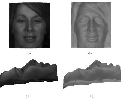
Some of the reconstructed surfaces from the Agrawal et al. method are depicted in Figs. 4 and 5 in both frontal and profile view with and without the albedo. In the experimental results we have applied
well-known and standard techniques such as
VI. FACE RECOGNITION USING2DINTENSITY IMAGES,DEPTH MAPS AND NORMAL FIELDS
This section describes the different recognition algorithms we applied to the various modalities available
to us using the Photoface database. Two different modalities are retrieved by the pipeline of PS: the albedo
A. Face recognition/verification using Albedo Images
Two well-established families of techniques were applied for this paper. The first one considers facial
images as vectors and finds linear projections for dimensionality reduction and feature extraction [30],
[31]. The other one is based on elastic graph matching [34]. We performed our experiments under two
distinct paradigms: in the first, we use only one sample for training and in the second we use two samples.
1) Subspace Methods based on Linear Projections: This family of methods aims to extract features using linear projections and includes PCA (Eigenfaces) [47], Nonnegative Matrix Factorization (NMF)
[48], Independent Component Analysis [49], etc. In our experiments NMF produced the best recognition
and verification results. In subspace methods such as NMF, the facial images are lexicographically scanned
so that the pixel values are re-shaped into vectors. LetM be the number of samples in the image database U = {u1,u2, ..,uM} where ui ∈ ℜn is a database image. A linear transformation of the original n
-dimensional space onto a subspace with m-dimensions (m ≪ n) is a matrix WT ∈ ℜm×n. The new
feature vectorsyk ∈ℜm are given by:
yk =WT(uk−u), k¯ ∈{1,2, . . . , M} (10)
whereu¯ ∈ℜn is the mean image of all samples. Classification is then performed using a simple distance
measure and a nearest neighbour classifier using the normalized correlation.
For the second testing paradigm, where we have two samples per person for training and one for
testing, we have also applied discriminant methods for recognition. In particular, we use the well-known
Linear Discriminant Analysis (LDA) method. We have considered five different approaches:
1) Fisherfaces [30]
2) PCA plus LDA [50] where we have two different spaces the regular and irregular,
3) an LDA method based on a slightly different criterion [51]
4) LDA method proposed in [52] which uses a regularization on the eigenspectrum
5) NMF plus LDA [31], [53].
The interested reader may refer to [30], [50], [51], [52], [31], [53] for details regarding the algorithms.
In our experiments here, most of the discriminant approaches resulted in very similar recognition rates.
For the sake of compactness therefore, we shall only detail results of the NMF+LDA approach.
2) Elastic (Bunch) Graph Matching: The second family of techniques that we applied is that of Elastic Graph Matching (EGM) or Elastic Bunch Graph Matching (EBGM). In the first step of the EGM
algorithm, a suitable face representation based on a sparse graph is selected. A uniformly distributed
rectangular graph is one of the simplest forms possible. For this case, only a face detection algorithm is
required in order to find an initial approximation of the desired rectangular facial region. An example of
such a reference graph is depicted in Fig. 6.
In the second step the facial image region is analyzed and a set of local descriptors is extracted at each
graph node (called jets). Analysis is usually performed by building an information pyramid using
outputs of multiscale morphological dilation-erosion operations or the morphological signal decomposition
at several scales are nonlinear alternatives of the Gabor filters for multiscale analysis. Both have been
successfully used for facial image analysis [54]. Morphological feature vectors have the advantage of
robustness to plane rotations. A robust to rotation and scaling jet based on Gabor filters was recently
proposed in [55].
The third step involves matching the reference graph on the test face image in order to find the
correspondences of the reference graph nodes on the test image. This is accomplished by minimizing a
cost function that employs node jet similarities while simultaneously preserving the node neighbourhood
relationships.
Due to the matching procedure, EGM algorithms are relatively robust against facial image
misalign-ment. Moreover, due to local node deformations, EGM algorithms are also relatively robust against the
presence of facial expressions. In order to further boost the performance of EGM, subspace methods can be
applied to extract features from the graphs, as in [34], [33], [32], [56]. We have applied many unsupervised
and supervised dimensionality reductions on the graphs to increase recognition speed (e.g. PCA, ICA,
NMF) but for consistency and compactness we only report the results based on NMF and NMF plus
LDA.
B. Face recognition using Depth Images and Normals
We perform face recognition on the surface normal estimates (as described in Section IV) and using
depth images that were computed by the integration of the normal field (as described in Section V). We
mainly experimented with recognition/verification methods that process the depth maps in exactly the
same manner as the intensity images. That is, we applied dimensionality reduction methods based on
linear projections and EGM algorithms. For the latter we used multiscale log-Gabor filters, which have
been shown to be quite useful for processing of depth images [57], in order to fill the jets of the graphs.
Finally, we applied a method [34] that operates on the intensity images but uses the 3D information
for more reliable matching. In particular, in [34], an EGM algorithm was proposed which exploits the
information of the 3D depth maps only in the matching process. Instead of using the simple distance on
a 2D grid, the nodes are mapped on the 3D surface. The method then uses geodesic distances between
nodes as a similarity measure. For this paper, the geodesic distances between the points were calculated
using the depth map derived from PS. Moreover, they are robust against isometry mappings (or isometries)
of the facial surfaces. The facial pose variations are isometries of the facial surfaces and, to an extent,
so are facial expressions (as long as the mouth remains closed). That is, the geodesic distances before
and after the development of an expression are considered to remain (approximately) identical [58]. An
example of matching using the algorithm in [34] can be seen in Fig. 7 where the final node positions
C. Face Recognition using NormalFaces
The final modality for face recognition we consider in this paper is based on the orientation of the
normals. The baseline method is straightforward to implement and is based on a novel representation of
faces: the so-called “Normalfaces”. For an image I using the computed P and Q from PS (5–??) we
compute:
Φ(x) =atanQ(x)
P(x) (11)
which is an image that contains the normal orientations. Example normal orientation images are shown
in Fig. 8.
We measure the orientations in the interval ∈ [−π2,π2]. For two images Φ1(x) and Φ2(x) we use the
following dissimilarity measure:
d(Φ1(x),Φ2(x)) = 1−
1 N M π
N∑×M
i=1
|Φ1(xi)−Φ2(xi)|. (12)
This dissimilarity measure can be transformed to a kernel and then used to extract features using
embedding as described in [59]. This kernel can be also used for extracting discriminant features using
kernel Fisherfaces [60]. Classification is performed using the normalized correlation in the new
low-dimensional space.
VII. EXPERIMENTALRESULTS
The results presented in this section are divided into recognition and verification. For each case we
present results for albedo, surface normals, depth and fusion of 2D and 3D data. In particular we present
experiments using Single Sample Single Modality (SSSM), Single Sample Multiple Modalities (SSMM)
and Multiple Sample Single Modality (MSSM) [35].
A. Recognition Experiments
For these experiments, we used a subset of 126 subjects taken with more than a week’s interval. For
the majority of them (90 subjects) the interval was greater than one month. For the experiments presented
here we tested using two set-ups:
• In the first one, a very challenging experimental procedure was followed, exploiting only one grayscale albedo image or surface normal map obtained from PS, or the depth image derived from
the integration of the normal field. Similarly, one albedo image, normal map or height map was
used for testing. Most of the training and testing images display a different facial expression. This
one-sample face recognition challenge is one of the most difficult scenarios in the field and has
various applications [61]. Related one-sample experiments can be found in [4], [18], [35].
TABLE I
ASUMMARY OF THE BEST(ACCORDING TO THE DIMENSIONS KEPT) PERCENTAGE OFRECOGNITION(PR)FOR ALBEDO
IMAGES FOR THE FIRST EXPERIMENTAL SET-UP(ONE-SAMPLE).
Method 4LPS (%) 3LPS (%) RPS (%) 3LPS-OPT (%)
SUB 78 74 78 72.5
EGM-SUB 82.5 79 82.5 80
the same as that used in the one-sample experimental set-up. This is in order to test whether or
not recognition using two samples of the same modality is better than fusing information across
different modalities. (We also check results using these 96 subjects for the one-sample setup).
We also conducted the following set of experiments in order to justify why face recognition using PS
is useful we trained supervised and unsupervised subspace methods (such as NMF, PCA, LDA etc) and
Elastic Bunch Graph using jets using all four images with and without illumination compensation ([?],
[?], [?]) and fuse the results (with weighted and non weighted schemes). Furthermore, we also trained
unsupervised subspace learning methods per light and then fuse the scores per light. In all cases the
recognition rate achieved was never higher than the best recognition rate achieved by a single albedo
image and it is worth noting here that the application of discriminant subspace learning techniques (i.e.,
LDA) resulted in much poorer performance than using a single albedo images (something that has been
previously reported in the literature [62]). On the other hand, in the PS architecture except from the
albedo image we have also available the facial shape information, which when fused, as we show, (even
with very simple fusion rules), achieves much better performance than the single albedo image.
Finally, we note that in the following the reported recognition rates are rounded to .0 or 0.5 based on
what is closer.
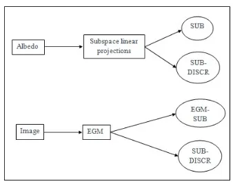
1) Albedo Images: Four source, three source, optimal three source (optimal according to [40]) and ray trace-based PS methods were employed for albedo computation. These methods are abbreviated as 4L-PS
[38], 3L-PS [38], 3L-OPT [40] and RAY-PS [39], respectively. The recognition results of the subspace
methods are abbreviated as SUB (i.e., NMF), while EGM methods using subspaces for boosting the
performance are abbreviated as EGM-SUB (the pipeline of the methods used for recognition in the albedo
and depth images can be seen in Fig. VI-C, along with their acronyms. Table I shows the recognition
rates for each method on this one-sample set-up. Note that the recognition rate is affected by the PS
method applied and noticeably better recognition performance is achieved by PS methods that use all
four illuminants. The best recognition rate was equal to 78% for the SUB methods and 82.5% for the
EGM-SUB method (the improvement is mainly due to the alignment step in the EGM algorithm).
For the case of the two-sample experiment, we used two different approaches:
TABLE II
ASUMMARY OF THE BESTPRFOR ALBEDO IMAGES FOR THE SECOND EXPERIMENTAL SET-UP(TWO-SAMPLE).
Method 4LPS (%) 3LPS (%) RPS (%) 3LPS-OPT (%)
EGM-DISCR 95 91.5 95 93.5
SUB-DISCR 92.5 86.5 89.5 88.5
EGM-SUB 87.5 84 88 86.5
SUB 85 80 85.5 84.5
TABLE III
ASUMMARY OF THE BESTPRFOR DEPTH IMAGES USING SUBSPACE ALGORITHMS FOR THE FIRST EXPERIMENTAL SET-UP.
Method 4LPS (%) 3LPS (%) RPS (%) 3LPS-OPT (%)
AT 59.5 58.5 60 59
DCTFC 74 67 72.5 70
FC 65.5 64 67 65
LS 63.5 60 64 66.5
ME 65.5 59.5 64 67
two samples of 2D albedo images and ranked the subjects based on the combined scores. Scores
from each modality are linearly normalized to the range of [0; 100] before combining. We explored
various confidence-weighted versions of the sum, product and minimum rules. However the simple
sum rule provided the best overall performance.
• Secondly, we applied supervised SUB (i.e., NMF plus LDA) and EGM methods, abbreviated to SUB-DISCR and EGM-DISCR respectively (DISCRiminant). In this case, the second sample is
used for learning discriminant projections and we classify using the minimum between the two
distances.
The recognition rates for these two-sample experiments for all PS algorithms is summarized in Table
II. As can be seen, the use of more than one sample increases the recognition performance. Moreover,
the methods which use all four illuminants achieved better recognition rates than those using only three,
as before. The best recognition rate was to 95%.
It is important to note that the recognition rate when using only the 96 subjects of the second experiment
in the one-sample tests, the recognition rate was also about 78%and 82.5%. Note the major improvement
of over 10% between the one-sample tests and the two-sample tests. As an extra verification of this, we
repeated the one-sample test using only the 96 subjects of the two-sample test and obtained similar
results.
2) Depth Images and Normal Orientations: We applied five different methods for surface reconstruc-tion from the normal field. For the reconstrucreconstruc-tion methods we use the following abbreviareconstruc-tions: 1) ’AT’
TABLE IV
ASUMMARY OF THE BESTPRFOR DEPTH IMAGES USINGEGMALGORITHM FOR FIRST EXPERIMENTAL SET-UP.
Method 4LPS (%) 3LPS (%) RPS (%) 3LPS-OPT (%)
AT 70 61 67 63
DCTFC 79 72 77.5 74.5
FC 74 67 71 70
LS 73 68 70 68
ME 73.5 68.5 67.5 68
TABLE V
ASUMMARY OF THE BESTPRFOR DEPTH IMAGES USING SUBSPACE ALGORITHMS AND FUSION FOR THE SECOND
EXPERIMENTAL SET-UP.
Method 4LPS (%) 3LPS (%) RPS (%) 3LPS-OPT (%)
AT 81 80 81 80
DCTFC 86.5 84 85.5 85.5
FC 82 82 81 81
LS 80 78 81 78
ME 79 78 81 78
3) FC for the original Frank-Chellappa method [64], 4) ’LS’ for the least square solution of the poison
equation [43] and 5) ’ME’ for the reconstruction based on M-estimator [45]. The recognition rates for
the one-sample experiment and for all reconstruction and PS methods are summarized in Table III for
SUB methods and Table IV for EGM-SUB.
The best recognition result acquired was 74% for SUB and 79% for EGM-SUB. As can be seen,
PS and reconstruction methods greatly affect the recognition performance. More precisely, four source
PS methods always achieve better recognition results, which is conducive to the albedo image tests.
Moreover, the depth maps that were produced by DCTFC constantly outperformed the PR of the depth
maps produced by all other reconstruction methods. The best results for the case of albedo in the
similar experimental setting was 78% for SUB and 82.5%. Hence, there is a difference of 4% and
3.5%, respectively. This is attributed to the error in reconstruction.
Experiments using two samples for training and one sample for testing are summarized in Tables V,
VI, VII and VIII for SUB, EGM-SUB, SUB-DISCR and EGM-DISCR, respectively. The same methods
as those used in case of albedo were applied in these experiments for fusion and classification. As can
also be observed, we can verify the finding of the first experiment where the images produced by 4
source PS methods and DCT-based FC surface reconstruction methods constantly outperform all other
methods.
The experiments using the NormalFace approach for all tested PS methods are summarized in Table IX
TABLE VI
ASUMMARY OF THE BESTPRFOR DEPTH IMAGES USINGEGMALGORITHMS AND FUSION FOR THE SECOND
EXPERIMENTAL SET-UP.
Method 4LPS (%) 3LPS (%) RPS (%) 3LPS-OPT (%)
AT 83 82 84.5 83
DCTFC 88 86 88 86.5
FC 84 82 83.5 83
LS 82 81.5 83.5 83
ME 82 81.5 82.5 83
TABLE VII
ASUMMARY OF THE BESTPRFOR DEPTH IMAGES USING DISCRIMINANT SUBSPACE ALGORITHMS FOR THE SECOND
EXPERIMENTAL SET-UP.
Method 4LPS (%) 3LPS (%) RPS (%) 3LPS-OPT (%)
AT 91 86 92 87
DCTFC 94 89 94.5 90.5
FC 93 87.5 92.5 89.5
LS 89 85 88.5 85
ME 88 84 87 85.5
kernel framework for feature extraction [59] using the proposed distance in (12). For the 2Tr.-Discr setting
we used the same framework as in 1 Tr. and then LDA on the produced features. For the two-sample
experiments fusion experiments, the same fusion strategy was applied to that in the albedo experiment
(2Tr.-Fuse).
A summary of the best results from all the modalities is given in Tables XXI. From the summary we
can deduce the following
• in the one sample experiment, the use of albedo produces better results than normal and depth • in the two sample experiment all modalities have similar performance
TABLE VIII
ASUMMARY OF THE BESTPRFOR DEPTH IMAGES USINGEGMALGORITHMS AND DISCRIMINANT SUBSPACE METHODS
FOR THE SECOND EXPERIMENTAL SET-UP.
Method 4LPS (%) 3LPS (%) RPS (%) 3LPS-OPT (%)
AT 93 89 93 90
DCTFC 96 92 96 93
FC 96 92 94 92
LS 93 89 92 90
TABLE IX
ASUMMARY OF THE BEST RECOGNITION RATE FORNORMALFACE AND ALL THE TESTED METHODS FOR BOTH
EXPERIMENTS
Exp. 4LPS (%) 3LPS (%) RPS (%) 3LPS-OPT (%)
1Tr. 76 72 78 73
2Tr.-Fuse 86 82 86 82
2Tr.-Discr 96 89 95 90.5
TABLE X
ASUMMARY OF THE BESTPRFOR ALL THE CONDUCTED EXPERIMENTS ACROSS DIFFERENT MODALITIES.
Recognition (PR%)
One Sample Two Samples Albedo Depth Normal Albedo Depth Normal
82.5 79 78 95 96 95
• there is no difference in performance between the depth and normals.
We have to note that these conclusions refer only to the applied methods.
3) Fusion 2D and 3D data: Multimodal decision fusion was performed by combining the match scores for each person across the modalities of 2D albedo and depth image and ranking the subjects based on the
combined scores in a similar manner as in the two-sample experiments above. The sum rule provided the
best performance as before. We performed fusion only on depth images derived from DCTFC method and
4LPS as these gave best results in the earlier experiments. Fusion of intensity and geometry information
was conducted only on the subset of subjects that have more than 2 samples available in order to be
directly comparable to the single-modality two-sample experiments. In Table XI we summarize the best
results of the one sample experiments (i.e., SSSM and SSMM experimental setups) in order to highlight
the advantage of fusing 2D and 3D information. As can be seen the fusion of 2D and 3D improves
significantly the recognition rate.
The recognition results from multimodal fusion (in both SSMM and MSSM setups) using SUB methods
and EGM-DISCR, which achieved the best results, is given in Table XII.
TABLE XI
ASUMMARY OF THE BESTPRFOR ALL THE CONDUCTED EXPERIMENTS ACROSS DIFFERENT MODALITIES.
Recognition (PR%) One Sample Albedo Depth Normal Albedo plus Depth
TABLE XII
ASUMMARY OF THE BESTPRFOR FUSION ACROSS DIFFERENT SAMPLES AND MODALITIES.
Recognition (PR%)
Sample Fusion Modality Fusion Method Albedo Depth Normal Albedo + Depth
SUB 85 86 86 85
EGM-SUB 88 88 - 89
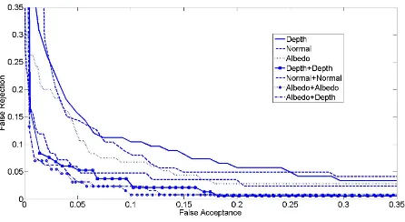
B. Verification Experiments
Face verification systems aim to determine whether or not an identity claim is valid. The performance
of face verification systems is typically measured in terms of the False Rejection Rate (FRR) achieved
at a fixed False Acceptance Rate (FAR). There is a trade-off between FAR and FRR. This trade-off
between the FAR and FRR can create a Receiver Operating Characteristic (ROC), where FRR is plotted
as a function of FAR. The performance of a verification system is often quoted by a particular operating
point of the ROC curve where FAR=FRR. This operating point is called Equal Error Rate (EER) and is
a useful scalar figure of merit commonly adopted to quantify verification performance. In the verification
experiments, we used the same matching score generators to those used in the recognition experiments
The verification protocol used in this paper is similar to the one defined in the FERET verification
protocol [65]. The test (or client) set was defined by the same 126 persons as in the above recognition
experiments. The first image per subject is used for training while the second is used for testing client
claims. The unused 135 people in the database, with one image per person, are considered to be impostors.
In a second verification experiment, we used two images from the 96 subjects for training while the
third is used for testing client claims. Again, the latter 135 persons were used for impostor claims.
1) Face Verification using Albedo, Depth and Normalface Images: The EERs for albedo data calcu-lated using the various PS methods for the one-sample experiment are summarized in Table XIII. The
corresponding results for the two-sample experiments are then summarized in Table XIV.
The EERs for various PS and surface reconstruction methods for the one-sample experiment are
summarized in Tables XV and XVI for SUB and EGM-SUB methods, respectively. The verification
results for the two-sample experiment and for various PS and surface reconstruction methods are depicted
in Tables XVII, XVIII, XIX and XX for SUB, EGM-SUB, SUB-DISCR and EGM-DISCR, respectively.
The EERs for various PS methods for the one-sample experiment for the case of Normalfaces are
summarized in Table XX. The corresponding verification results for the two-sample experiments and for
various PS methods are summarized in Table XXI (for the verification experiments the difference in EER
between fusion and discriminant learning was negligible hence for reasons of compactness we report
only the discriminant learning results).
TABLE XIII
ASUMMARY OF THE BESTEERFOR ALBEDO IMAGES FOR THE FIRST EXPERIMENTAL SET-UP.
Method 4LPS (%) 3LPS (%) RPS (%) 3LPS-OPT (%)
SUB 7.8 8 7.4 7.9
EGM-SUB 6.7 7.1 6.4 6.7
TABLE XIV
ASUMMARY OF THE BESTEERFOR ALBEDO IMAGES FOR THE SECOND EXPERIMENTAL SET-UP.
Method 4LPS (%) 3LPS (%) RPS (%) 3LPS-OPT (%)
EGM-DISCR 3.9 4.2 3.2 4.8
SUB-DISCR 4.4 4.7 3.8 5.2
EGM-SUB 5 6.4 4.3 6
SUB 5.8 7.3 5.3 6.2
TABLE XV
ASUMMARY OF THE BESTEERFOR DEPTH IMAGES USINGEGMALGORITHM FOR THE FIRST EXPERIMENTAL SET-UP.
Method 4LPS (%) 3LPS (%) RPS (%) 3LPS-OPT (%)
AT 12.1 13.7 12 12.4
DCTFC 8.8 11.4 9.9 10.7
FC 11 12.8 11.3 11.5
LS 10.7 12.8 10.7 11.9
ME 11.9 12.9 11.4 12
TABLE XVI
ASUMMARY OF THE BESTEERFOR DEPTH IMAGES USING SUBSPACE ALGORITHMS FOR THE FIRST EXPERIMENTAL SET-UP.
Method 4LPS (%) 3LPS (%) RPS (%) 3LPS-OPT (%)
AT 14.1 17.3 14.1 14.7
DCTFC 10.5 13.5 11.5 12.5
FC 13 15 13.1 13.7
LS 13 15.5 13.7 14.6
ME 13.9 15.4 14.4 14.9
TABLE XVII
ASUMMARY OF THE BESTEERFOR DEPTH IMAGES USING SUBSPACE ALGORITHMS AND FUSION FOR THE SECOND
EXPERIMENTAL SET-UP.
Method 4LPS (%) 3LPS (%) RPS (%) 3LPS-OPT (%)
AT 7.2 9.3 7.3 7.8
DCTFC 5.7 7.8 6 6.3
FC 7.2 10.2 8.4 8.6
LS 7.1 11.3 8.4 8.7
TABLE XVIII
ASUMMARY OF THE BESTEERFOR DEPTH IMAGES USINGEGMAND FUSION FOR THE SECOND EXPERIMENTAL SET-UP.
Method 4LPS (%) 3LPS (%) RPS (%) 3LPS-OPT (%)
AT 7.2 9.7 8.1 8.2
DCTFC 5 6.9 5.2 5.7
FC 6.7 9.6 7.3 7.5
LS 6.9 9 6.8 7.7
ME 6.7 8.5 6.5 8
TABLE XIX
ASUMMARY OF THE BESTEERFOR DEPTH IMAGES USING DISCRIMINANT SUBSPACE METHODS AND FUSION FOR THE
SECOND EXPERIMENTAL SET-UP.
Method 4LPS (%) 3LPS (%) RPS (%) 3LPS-OPT (%)
AT 5 5.9 5.3 5.8
DCTFC 4.2 5.2 4.5 4.7
FC 4.8 5.6 4.9 5.1
LS 4.9 5.3 4.7 5.1
ME 4.9 5.7 4.7 5
2) Multimodal Fusion: Multimodal decision fusion was performed in exactly the same way as for the recognition experiments. That is, by combining the match scores for each person across the modalities
of 2D albedo image and depth map and ranking the subjects based on the combined scores. In Table
XXIII we summarize the best results of the one sample experiment (i.e., SSSM and SSMM experimental
setups) in order to highlight the advantage of fusing 2D and 3D information. As can be seen the fusion
of 2D and 3D improves significantly the verification accuracy.
A summary of the best verification results for both the single modalities and multimodal fusion (in
both SSMM and MSSM setups) is given in Table XXIV.
TABLE XX
ASUMMARY OF THE BESTEERFOR DEPTH IMAGES USINGEGMAND DISCRIMINANT SUBSPACE METHODS FOR THE
SECOND EXPERIMENTAL SET-UP.
Method 4LPS (%) 3LPS (%) RPS (%) 3LPS-OPT (%)
AT 4.4 5 4.6 4.6
DCTFC 3.5 4.1 3.7 3.9
FC 4.1 4.6 4.2 4.3
LS 4.1 5 4.5 4.3
TABLE XXI
ASUMMARY OF THE BESTEERFORNORMALFACE AND ALL THE TESTED METHODS FOR BOTH EXPERIMENTS
Exp. 4LPS (%) 3LPS (%) RPS (%) 3LPS-OPT (%)
1Tr. 9 10.4 8.9 10.1
2Tr. 3.7 4.6 3.9 4.5
TABLE XXII
ASUMMARY OF THE BEST PERCENTAGE OFEERFOR ALL THE CONDUCTED EXPERIMENTS ACROSS DIFFERENT
MODALITIES.
Verification (EER%)
One sample Two samples Albedo Depth Normal Albedo Depth Normal
7.4 10.5 9.1 3.2 3.5 3.0
VIII. DISCUSSION ANDCONCLUDINGREMARKS
In this paper, we presented a new database collected in a real-life commercial setting based on PS.
We presented the first experiments which demonstrate how different methods in the pipeline of PS affect
the recognition performance and concluded the following:
• Four source PS methods produce facial samples (albedo, normals) that achieve constantly better recognition and verification performance than 3 source PS regardless of the reconstruction methods
applied.
• The reconstruction methods greatly affect the recognition and verification performance. The method
TABLE XXIII
ASUMMARY OF THE BESTPRFOR ALL THE CONDUCTED EXPERIMENTS ACROSS DIFFERENT MODALITIES.
Recognition (PR%) One Sample Albedo Depth Normal Albedo plus Depth
7.4 10.5 9.1 4.6
TABLE XXIV
ASUMMARY OF THE BEST PERCENTAGE OFEERFOR FUSION ACROSS DIFFERENT SAMPLES AND MODALITIES.
Verification (EER%)
Sample Fusion Modality Fusion Method Albedo Depth Normal Albedo + Depth
SUB 5.2 5.7 5.2 5.2
which constantly produces the best recognition/verification performance proved to be the one
pro-posed in [8], i.e. DCTFC.
Moreover, we have verified most of the following findings of [35]:
• In most cases, the best recognition and verification results using the recovered albedo, normals and reconstructed depth maps are approximately the same (there is difference in the one sample
experiment). In some cases, the recovered albedo produces better results.
• Fusion of the 2D (albedo) and 3D (depth or normal) information produce significantly better results than using either albedo or the depth image.
• Fusion of multiple albedo images and/or reconstructed surfaces produce significantly better results than using only one albedo or the depth image.
• Fusion of two albedo images (Single-Modality and Multiple-Sample (SMMS)) in the same way that we fused the results of albedo and depth map (Multiple-Modality and Single-Sample (MMSS)) gave
approximately the same recognition and verification performance. The major advantage of MMSS
over SMMS is that SMMS requires two recording sessions while MMSS only one.
The best recognition for any of the presented algorithms under the one-sample set-up was 86% and for the
two-sample was 96%. The corresponding verification experiments resulted in 6.4% for the one sample
experiment and 3.2% for the two sample experiment. The verification experiments show that there is
much space for improvement.
The database is available to the public by visiting
http://Photoface.iti.gr/ or http://www.uwe.ac.uk/research/Photoface.
ACKNOWLEDGMENTS
We would like to thank our colleagues at General Dynamics UK for their assistance in data capture
for this study.
REFERENCES
[1] S. Zafeiriou, M. Hansen, G. Atkinson, V. Argyriou, M. Petrou, M. Smith, and L. Smith, “The photoface database,”,” in
Proc. CVPR Workshop on Biometrics, Colorado Springs, Colorado, USA, 2011, pp. 161–168.
[2] R. J. Woodham, “Photometric method for determining surface orientation from multiple images,” Optical Engineering, vol. 19, pp. 139–144, 1980.
[3] S. Li and A. Jain, Handbook of Face Recognition, Springer-Verlag, 2005.
[4] P. J. Phillips, H. Wechsler, and P. Rauss, “The feret database and evaluation procedure for face-recognition algorithms,”
Image and Vision Computing, vol. 16, pp. 295–306, 1998.
[5] T. Sim, S. Baker, and M. Bsat, “The cmu pose, illumination, and expression database,” IEEE Trans. Patt. Anal. Mach. Intell., vol. 25, pp. 1615–1618, 2003.
[6] P. W. Hallinan, G. G. Gordon, A. L. Yuille, P. Giblin, and D. Mumford, Two- and Three- Dimensional Patterns of the Face, A K Peters Ltd., 1999.
[8] A. S. Georghiades, P. N. Belhumeur, and D. J. Kriegman, “From few to many: illumination cone models for face recognition under variable lighting and pose,” IEEE Trans. Patt. Anal. Mach. Intell., vol. 23, pp. 643–660, 2001.
[9] P. N. Belhumeur, J. P. Hespanha, and D. J. Kriegman, “Eigenfaces vs. fisherfaces: recognition using class specific linear projection,” IEEE Trans. Patt. Anal. Mach. Intell., vol. 19, pp. 711–720, 1997.
[10] K.C. Lee, J. Ho, and D. Kriegman, “Acquiring linear subspaces for face recognition under variable lighting,” IEEE Trans. Pattern Anal. Mach. Intelligence, vol. 27, no. 5, pp. 684–698, 2005.
[11] R. Gross, I. Matthews, J. Cohn, T. Kanade, and S. Baker, “Multi-pie,”Image and Vision Computing, vol. 28, pp. 807–813,
2010.
[12] G.B. Huang, M. Ramesh, T. Berg, and E. Learned-Miller, “Labeled faces in the wild: A database for studying face
recognition in unconstrained environments,” University of Massachusetts, Amherst, Technical Report 07, vol. 49, pp. 1, 2007.
[13] C. Beumier and M. Acheroy, “Face verification from 3d and grey level clues,” Pattern Recognition Letters, vol. 22, no. 11, pp. 1321–1329, 2001.
[14] C. Beumier and M. Acheroy, “Sic db: multi-modal database for person authentication,” 1999, pp. 704–708.
[15] A. Savran, N. Alyuz, H. Dibeklioglu, O. Celiktutan, B. Gokberk, B. Sankur, and L. Akarun, “Bosphorus database for 3d face analysis,” 2008, pp. 47–56.
[16] York 3D database, ,” 2011.
[17] T. Heseltine, N. Pears, and J. Austin, “Three-dimensional face recognition using combinations of surface feature map
subspace components,”Image and Vision Computing, vol. 26, no. 3, pp. 382–396, 2008.
[18] P. Phillips, P. Flynn, T. Scruggs, K. Bowyer, J. Chang, K. Hoffman, J. Marques, J. Min, and W. Worek, “Overview of the
face recognition grand challenge,” inIn Proc. CVPR, 2005, pp. 947–954.
[19] T. Faltemier, K. Bowyer, and P. Flynn, “Using multi-instance enrollment to improve performance of 3d face recognition,” 2008, vol. 112, pp. 114–125.
[20] www.konicaminolta.com/sensingusa/products/3d/non contact/vivid910, “[Accessed 15 Dec 2009],” .
[21] C. Zhong, Z. Sun, and T. Tan, “Robust 3d face recognition using learned visual codebook,” 2007, pp. 1–6.
[22] Casia 3D face database, ,” 2011.
[23] A. Moreno and A. Sanchez, “Gavabdb: a 3d face database,” 2004, pp. 75–80.
[24] L. Yin, X. Chen, Y. Sun, T. Worm, and M. Reale, “A high-resolution 3d dynamic facial expression database,” 2008, pp.
1–6.
[25] L. Yin, X. Wei, Y. Sun, T. Worm, J. Wang , and M. Rosato, “A 3d facial expression database for facial behavior research,” 2006, pp. 211–216.
[26] Texas 3D Face Recognition Database, ,” 2010.
[27] S. Gupta, M.K. Markey, and A.C. Bovik, “Anthropometric 3d face recognition,”International journal of computer vision,
vol. 90, no. 3, pp. 331–349, 2010.
[28] www.3dmd.com/3dmdface.html, “[Accessed 13 March 2010],” .
[29] P. Tan, S. Lin, and L. Quan, “Subpixel photometric stereo,” IEEE Transactions on Pattern Analysis and Machine
Intelligence, pp. 1460–1471.
[30] P. N. Belhumeur, J. P. Hespanha, and D. J. Kriegman, “Eigenfaces vs. Fisherfaces: Recognition using class specific linear
projection,” IEEE Transactions on Pattern Analysis and Machine Intelligence, vol. 19, no. 7, pp. 711–720, July 1997.
[31] S. Zafeiriou, A. Tefas, I. Buciu, and I. Pitas, “Exploiting discriminant information in nonnegative matrix factorization with
application to frontal face verification,”IEEE Transactions on Neural Networks, vol. 17, no. 3, pp. 683 – 695, 2006.
[32] S. Zafeiriou, A. Tefas, and I. Pitas, “Learning discriminant person specific facial models using expandable graphs,” IEEE
Transactions on Information Forensics and Security, vol. 2, no. 1, pp. 50–55, Mar. 2007.
[34] S. Zafeiriou and M. Petrou, “2.5d elastic graph matching,” Computer Vision and Image Understanding, vol. 115, no. 7, pp. 1062–1072, July 2011.
[35] K.I. Chang, K.W. Bowyer, and P.J. Flynn, “An evaluation of multimodal 2D+ 3D face biometrics,”IEEE Transactions on
Pattern Analysis and Machine Intelligence, pp. 619–624, 2005.
[36] B. Gokberk, H. Dutagaci, A. Ulas, L. Akarun, and B. Sankur, “Representation plurality and fusion for 3-D face recognition,”
IEEE Transactions on Systems Man and Cybernetics-Part B-Cybernetics, vol. 38, no. 1, pp. 155–173, 2008.
[37] R. Lienhart and J. Maydt, “An extended set of Haar-like features for rapid object detection,” inIEEE ICIP, 2002, pp. 900–903.
[38] D. A. Forsyth and J. Ponce, Computer Vision, A Modern Approach, Prentice Hall, Upper Saddle River, NJ, 2003.
[39] V. Argyriou and M. Petrou, “Recursive photometric stereo when multiple shadows and highlights are present,” in
Proceedings of IEEE Conference on Computer Vision and Pattern Recognition, 2008, pp. 1–6.
[40] Mark F. Hansen, Gary A. Atkinson, Lyndon N. Smith, and Melvyn L. Smith, “3D face reconstructions from photometric stereo using near infrared and visible light,”Comp. Vis. Im. Understanding, vol. to appear.
[41] R.T. Frankot and R. Chellappa, “A method for enforcing integrability in shape from shading algorithms,”IEEE Transactions on Pattern Analysis and Machine Intelligence, vol. 10, no. 4, pp. 439–451, 1988.
[42] A.S. Georghiades, P.N. Belhumeur, and D.J. Kriegman, “From few to many: Illumination cone models for face recognition
under variable lighting and pose,” IEEE Transactions on Pattern Analysis and Machine Intelligence, vol. 23, no. 6, pp. 643–660, 2001.
[43] T. Simchony, R. Chellappa, and M. Shao, “Direct analytical methods for solving Poisson equations in computer vision problems,” IEEE Transactions on Pattern Analysis and Machine Intelligence, vol. 12, no. 5, pp. 435–446, 1990.
[44] A. Agrawal, R. Chellappa, and R. Raskar, “An algebraic approach to surface reconstruction from gradient fields,” inProc.
Intl Conf. Computer Vision, 2005, vol. 1, pp. 174–181.
[45] A. Agrawal, R. Raskar, and R. Chellappa, “What is the range of surface reconstructions from a gradient field?,” Lecture Notes in Computer Science (European Conference on Computer Vision (ECCV 2006) ), vol. 3951, pp. 578, 2006.
[46] BKP Horn and MJ Brooks, “Shape and source from shading,” inInternational Joint Conference on Artificial Intelligence, 1985, pp. 932–936.
[47] M. Turk and A. P. Pentland, “Eigenfaces for recognition,” Journal of Cognitive Neuroscience, vol. 3, no. 1, pp. 71–86,
1991.
[48] D.D. Lee and H.S. Seung, “Algorithms for non-negative matrix factorization,” inNIPS, 2000, pp. 556–562.
[49] M.S. Bartlett, J.R. Movellan, and T.J. Sejnowski, “Face recognition by independent component analysis,”IEEE Transactions on Neural Networks, vol. 13, no. 6, pp. 1450–1464, 2002.
[50] J. Yang, A.F. Frangi, J. Yang, D. Zhang, and Z. Jin, “KPCA plus LDA: A complete kernel Fisher discriminant framework for feature extraction and recognition,” IEEE Transactions on Pattern Analysis and Machine Intelligence, vol. 27, no. 2,
pp. 230–244, 2005.
[51] H. Li, T. Jiang, and K. Zhang, “Efficient and robust feature extraction by maximum margin criterion,”IEEE Transactions on Neural Networks, vol. 17, no. 1, pp. 157–165, Jan. 2006.
[52] X. Jiang, B. Mandal, and A. Kot, “Eigenfeature regularization and extraction in face recognition,” IEEE Transactions on Pattern Analysis and Machine Intelligence, vol. 30, no. 3, pp. 383–394, 2008.
[53] S. Zafeiriou, A. Tefas, and I. Pitas, “Discriminant nmf-faces for frontal face verification,” inIEEE International Workshop
on Machine Learning for Signal Processing, Mystic, Connecticut, 2005.
[54] C. Kotropoulos, A. Tefas, and I. Pitas, “Frontal face authentication using discriminating grids with morphological feature vectors,” IEEE Transactions on Multimedia, vol. 2, no. 1, pp. 14–26, Mar. 2000.
[55] H.-C. Shin, J.H. Park, and S.-D. Kim, “Combination of warping robust elastic graph matching and kernel-based projection
discriminant analysis for face recognition,” IEEE Transactions on Multimedia, vol. 9, no. 6, pp. 1125–1136, Oct. 2007.
[56] S. Zafeiriou, A. Tefas, and I. Pitas, “The discriminant elastic graph matching algorithm applied to frontal face verification,”