Numerical Solutions of the Modiﬁed Burger’s Equation using FTCS Implicit Scheme

(1)

Numerical Solutions of the Modified Burger’s

Equation using FTCS Implicit Scheme

Surattana Sungnul, Bubpha Jitsom and Mahosut Punpocha

Abstract—In this paper, we investigate the behavior of a modified Burger’s equation in the form

ut+ (c+bu)ux= (µ0+µ1u)uxx,

where c, b, µ0 and µ1 are arbitrary parameters. Numerical

solutions of this problem is obtained by the finite difference method in FTCS implicit scheme. The results obtained by advantages of mathematical software are compared between the numerical solutions and the exact solutions for some given initial and boundary conditions.

Index Terms—Burger’s equation, FTCS implicit scheme, finite difference method.

I. INTRODUCTION

B

URGER’S equation is a nonlinear partial differential equation, describing an evolutionary process in which a convective phenomenon is in balance with a diffusive phenomenon. The complete nonlinear Burger’s equation is given by [13]

∂u ∂t +u

∂u ∂x =µ0

∂2_u

∂x2,(x, t)∈D, (1) where uis fluid velocity, µ0 is viscosity coefficient and D is a continuous domain.

Equation (1) is a parabolic PDE, which can serve as a model equation for the boundary-layer equations. For the steady boundary-layer and ”parabolized” Navier-Stokes equation, the independent variables tandxcan be replaced byxand y, respectively to give

∂u ∂x+u

∂u ∂y =µ0

∂2_u

∂y2,(x, y)∈D, (2)

where x, y are the marching direction. For simplicity, the linear Burger’s equation

∂u ∂t +c

∂u ∂x =µ0

∂2_u

∂x2, (3)

is often used in place of equation (1). Note that if c = 0, equation (3) represents the heat equation. The exact steady-state solution of equation (3) with the boundary conditions,

u(0, t) =u0≡constant, (4)

u(l, t) = 0, (5)

is given by

u=u0

{

1−exp[Rl(x_l −1)] 1−exp(−Rl)

}

, (6)

Manuscript received June 16, 2017; revised October 31, 2017. S. Sungnul is a lecturer at the Department of Mathematics, King Mongkut’s University of Technology North Bangkok, 10800 THAILAND and a researcher in Centre of Excellence in Mathematics, 10400 THAI-LAND e-mail: [email protected].

B. Jitsom and M. Punpocha are in the Department of Mathematics, King Mongkut’s University of Technology North Bangkok, 10800 THAILAND e-mail: [email protected] and [email protected].

where

Rl= cl µ0 .

The exact unsteady solution of equation (3) and the initial condition [13] can be expressed as

u(x,0) =sin(kx),

where k is a constant. The periodic boundary condition is given by

u(x, t) =exp(−k2µ0t)sink(x−ct). (7)

Equations (1) and (3) can be combined into a generalized equation as

ut+ (c+bu)ux=µ0uxx, (8)

wherec andb are free parameters. Note that if b = 0, the linear equation is obtained. Moreover if c = 0 andb = 1, the nonlinear Burger’s equation is obtained. For the case that c = 1₂ and b = −1, the generalized Burger’s equation has the stationary solution

u=−c b

[

1 +tanhc(x−x0) 2µ0

]

. (9)

Hence, if the initial distribution of u is given by equation (9), the exact solution does not vary with time but it remains fixed at the initial distribution. Additional exact solution of Burger’s equation can be found by Platzman (1972), which describes 35 different exact solutions.

Equation (8) can be put into conservative form

ut+Fx= 0, (10)

whereF is defined by

F =cu+bu 2

2 −µ0ux. (11)

Alternatively, equation (8) can be rewritten as

ut+Fx=µ0uxx, (12)

whereF is defined by

F =cu+bu 2

2 . (13)

For the linearized case (b= 0),F is reduced into

F =cu.

In 2010, Blandin et al [1] considered the problem of sta-bilization of the inviscid Burgers equation using boundary conditions. Wu [2] suggested a fractional Lie group method to solve fractional partial differential equation. A time-fractional Burgers equation is used as an example to illustrate the effectiveness of the Lie group method and a few classes

IAENG International Journal of Applied Mathematics, 48:1, IJAM_48_1_08

(2)

of the exact solution were obtained. Pandey and Verma [3] generated the numerical solutions of the Burger’s equation by applying the Crank-Nicolson method directly to the Burger’s equation.

In 2012, Jiwari [4] used uniform Haar wavelet and the quasilinearization process to propose for the numerical sim-ulation of time dependent nonlinear Burgers equation. The following year, the study of a fractional Burgers equation arising in nonlinear acoustics was presented by Lombard, et al [5].

In 2014, Wongsaijai et al [6] proposed a compact finite difference method to solve the Rosenau-RLW equation. A numerical tool is applied to the model by using a three-level average implicit finite difference technique.

In 2015, other methods occurred, such as a fourth-order singly diagonally implicit runge-Kutta method for solving one-dimensional Burgers’ equation was presented by Deng and Pan [7]. A hybrid numerical scheme based on the Euler implicit method and quasilinearization. Uniform Haar wavelets was developed for the numerical solution of the Burgers equation by Jiwari [8]. Zhanlav et al [9] proposed an explicit finite difference scheme to solve the unsteady Burgers equation. Esen and Tasboza [10] presented a few numerical examples which supported numerical results for the time fractional Burgers equation, where various boundary and initial conditions obtained by collocation method using cubic B-spline. Bhrawy [11] reported a new space-time spectral algorithm to obtain an approximate solution for the space-time fractional Burger’s equation. The algorithm was based on a spectral shifted Legendre collocation method in combination with the shifted Legendre operational matrix of fraction derivatives.

In 2016, Seydaoglu et al [12] used a high order splitting method to calculate the numerical solution of the Burger’s equation in one dimensional space with periodic boundary conditions.

In this work, we study the modified Burger’s equation (8) with modified coefficient of viscosity as

ut+ (c+bu)ux= (µ0+µ1u)uxx, (14)

where the parametersc,b,µ0 and µ1 are given. Numerical solutions of the modified Burger’s equation are obtained by the finite difference method in FTCS implicit scheme.

II. CONVERGENCETHEORY

Here we consider boundary value problem (BVP) consist-ing of a partial differential equation with initial and boundary conditions

Lu=f, in domain D, (15)

and boundary condition isu(x, t) =υ(x, t)for(x, t)∈∂D, where L is differential operator acting from a space of continuous functions Ω to a continuous function space H (L: Ω→H).

We construct the grid Dh ∈ D ∪∂D and determine the linear space of discrete functionsΩhgiven on gridDh. Let us consider a finite difference scheme (FDS) which corresponds

and boundary condition is

uh(xi, tn) =υh(xi, tn)for (xi, tn)∈∂Dh,

Dh={(xi, tn)|i= 0,±1,±2, ..., M, n= 0,1, ...,[T /τ]−1},

τ is time step,whereLh is difference operator acting from a discrete function space Ωh to a discrete function space Hh (Lh: Ωh→Hh). Assuminguis a function ofxandt, we haveun

i =u(xi, tn)and denotefh,such that

fh=

{

φn i ψi

, i= 0,±1,±2, ..., M, n= 0,1, ...,[T /τ]−1,

where φn_i is function on the right hand side of FDS (16) andψi is value of initial condition.

To study stability of numerical methods we need to introduce the norms into the set of discrete functions

∥uh∥Ωh =maxi,n|uni|,

∥fh∥Hh =maxi|ψi|+maxi,n|φ n i|.

Lax’s equivalence theorem[13]

Given a properly posed boundary value problem and a fi-nite difference approximation to it that satisfies the consistent condition, stability is the necessary and sufficient condition for convergence.

1) Consistency: A finite difference representation of a

PDE is said to be consistent [13] if we should be able to show that the difference between the PDE and its difference representation vanishes as the mesh is refined, i.e., the truncation error (T.E.) goes to zero as the mesh size go to zero. This should always be the case if the order of the T.E.vanishes under grid refinement.

It is said that FDS (16) approximate with orderkof BVP (15) if

∥T.E.∥Hh ≤Ch

k _as _h_→₀_,

where the constantC does not depend on h.

2) Stability: The finite difference scheme defined by (16)

with linear operatorLhis called stable, if there existh0>0 such that for arbitraryh < h0 and for any discrete function fh_∈_H

h,the solution of FDS,uh, which satisfies

Lhuh=fh,

exists uniquely and satisfies the inequality

∥uh∥Ωh ≤C∥f h_∥

Hh, (17)

where the constant C does not depend on h. The scheme defined by (16) is called stable for(x, t)∈D∪∂D, if there exist a constantC independent ofhandτ such that

maxi,n|un_i| ≤C[maxi|ψi|+maxi,n|φni|], (18)

i= 0,±1,±2, .., M, n= 0,1, ...,[T /τ]−1.

The inequality (18) has to hold for any functionsψi andφni. For a particular case whenφn

i ≡0,we have only necessary condition for stability.

By Fourier or Von Neumann Analysis [13], we will seek solution to FDS (16) in the form

IAENG International Journal of Applied Mathematics, 48:1, IJAM_48_1_08

(3)

whereeIαi _{are eigenvectors corresponding to an eigenvalue} λandαis a wave number.

Necessary condition for stability of FDS (16) will be true for allα∈R which the following inequality (20) holds

|λ(α)|≤1. (20)

III. NUMERICALRESULTS

This section presents the examples of linear and nonlinear modified Burger’s equation (14).

A. Linear Burger’s equation

In the modified Burger’s equation (14) ifb= 0andµ1= 0 is called the linear Burger’s equation and written in the form

ut+cux=µ0uxx (21)

In paper [14], B. Jitsom and et. al presented that the numerical solution by FTCS implicit scheme converge to an exact solution. They found that FTCS implicit scheme has properties of consistency with T.E.=(O(∆t,(∆x)2₎)_and unconditional stability with

λ= 1

1 + 4Qsin2(α₂)+IPsinα,

then

|λ|=√[ 1

1 + 4Qsin2(α₂)]2+P2_sin2_α≤ 1,

whereP =c∆t_∆x andQ= µ0∆t

(∆x)2.

An example of linear Burger’s equation is shown in problem A1.

Problem A1: Let us consider linear Burger’s equation (22)

ut+ 1 10ux=

1

2uxx, 0≤x≤1, 0≤t≤1. (22) With initial condition :

u(x,0) = 1 2

[

1−tanh

{

1

2(x−15)

}]

,

and boundary conditions :

u(0, t) =1 2

[

1−tanh

{

1 2(15−

1 2t)

}]

,

u(1, t) =1

2[1−tanh(−7−t)]. Grid system :

Dh={(xi, tn)|xi= (i−1)∆x, tn= (n−1)∆t),

i= 1,2, ..., M, n= 1,2, ..., T}.

By FTCS implicit scheme, we have

un+1_i −un i

∆t +

1 10

un+1_i+1 −un+1_i₋₁ 2(∆x) −

1 2

un+1_i+1 −2un+1_i +un+1_i₋₁ (∆x)2 = 0,

(23)

u0_i =1 2

[

1−tanh

{

1

2(xi−15)

}]

,

un₁ =1 2

[

1−tanh

{

1 2(15−

1 2tn)

}]

,

un_M = 1

2[1−tanh(−7−tn)].

The exact solution of (22) with the initial and boundary conditions is

u(x, t) = 1 2

[

1−tanh

{

1

2(x−15− 1 2t)

}]

[image:3.595.352.501.66.143.2]

. (24)

Table I presents the absolute error between exact and nu-merical solutions of problem A1 with ∆t = ∆x = 0.05 and the graphs of exact solution and numerical solutions of linear Burger’s equation for FTCS implicit scheme are shown in Fig. 1 and Fig. 2 respectively. Moreover, The graph of absolute error between exact and numerical solutions of problem A1 is shown in Fig. 3. We can see that maximum of absolute error occurred at the middle spacexin each time stept.

TABLE I

ABSOLUTE ERROR BETWEEN EXACT AND NUMERICAL SOLUTIONS FOR

PROBLEMA1WITH∆t= ∆x= 0.05

t x

0.25 0.50 0.505 0.75

0 0.00 0.00 0.00 0.00

0.10 2.16×10−4 ₂_.₇₆_×₁₀−4 ₂_.₇₇_×₁₀−4 ₂_.₅₅_×₁₀−4

0.20 3.46×10−4 ₄_.₆₃_×₁₀−4 ₄_.₆₃_×₁₀−4 ₄_.₁₃_×₁₀−4

0.30 4.28×10−4 5.81×10−4 5.81×10−4 5.11×10−4 0.40 4.78×10−4 ₆_.₅₄_×₁₀−4 ₆_.₅₃_×₁₀−4 ₅_.₇₁_×₁₀−4

0.50 5.08×10−4 ₆_.₉₈_×₁₀−4 ₆_.₉₆_×₁₀−4 ₆_.₀₇_×₁₀−4

0.60 5.24×10−4 ₇_.₂₃_×₁₀−4 ₇_.₂₁_×₁₀−4 ₆_.₂₇_×₁₀−4

0.70 5.33×10−4 ₇_.₃₆_×₁₀−4 ₇_.₃₄_×₁₀−4 ₆_.₃₇_×₁₀−4

0.80 5.36×10−4 ₇_.₄₁_×₁₀−4 ₇_.₃₉_×₁₀−4 ₆_.₄₁_×₁₀−4

0.90 5.36×10−4 ₇_.₄₁_×₁₀−4 ₇_.₃₉_×₁₀−4 ₆_.₄₁_×₁₀−4

1.00 5.34×10−4 ₇_.₃₈_×₁₀−4 ₇_.₃₆_×₁₀−4 ₆_.₃₈_×₁₀−4

0 0.2

0.4 0.6

0.8 1

0 0.2 0.4 0.6 0.8 1 0.97 0.98 0.99 1

x Exact solutions of linear Burger’s equation

t

U(x,t)

Fig. 1. The plot of exact solution for Problem A1 withc= 1/10,b= 0and µ0= 1/2.

IAENG International Journal of Applied Mathematics, 48:1, IJAM_48_1_08

[image:3.595.44.545.318.738.2]

(4)

0 0.2

0.4 0.6

0.8 1

0 0.2 0.4 0.6 0.8 1 0.97 0.98 0.99 1

x

Numerical solutions of linear Burger’s equation

t

U(x

i

,t n

[image:4.595.63.262.55.204.2]

)

Fig. 2. The plot of numerical solutions for Problem A1 withc= 1/10, b= 0, µ0= 1/2,∆t= 0.05and∆x= 0.05.

0 0.2 0.4

0.6 0.8 1

0 0.2 0.4 0.6 0.8 1 0 2 4 6 8

x 10−4

x

Error between exact and numerical solutions of linear Burgers equation

t

[image:4.595.73.264.275.411.2]

Error

Fig. 3. The plot of absolute error between exact and numerical solutions for Problem A1.

TABLE II

MAXIMUM OF ABSOLUTE ERRORS FORPROBLEMA1WITH ∆x= ∆t= 0.05,0.01,0.005,0.001

∆x ∆t Maximum of absolute errors

0.05 0.05 7.162×10−3 0.01 0.01 7.141×10−3

0.005 0.005 6.979×10−3

[image:4.595.299.551.497.802.2]

0.001 0.001 7.178×10−4

Table II presents the maximum of absolute errors, we can see that maximum of absolute error goes to zero as the grid sizes∆xand∆t go to zero.

B. Nonlinear Burger’s equations

Nonlinear Burger’s equations are investigated by comparing the results between numerical solutions in FTCS implicit scheme and exact solutions. We then study the behaviour of solutions of modified Burger’s equation (14) as follows,

ut+ (c+bu)ux= (µ0+µ1u)uxx. (25)

In this work, nonlinear Burger’s equation of 3 cases are studied as follows,

with0≤µ1≤1,

Case B3 : Nonlinear modified Burger’s equation for stationary solution withµ1= 0.

Case B1: Nonlinear modified Burger’s equation in conser-vative form withµ1= 0.

We consider nonlinear generalized Burger’s equation (8) in the conservative form,

ut+Fx=µ0uxx where F =cu+ bu2

2 . (26) To obtain numerical solutions, we use FTCS implicit scheme as follows,

un+1_i −un i

∆t +

Fn

i+1−Fin₋1 2∆x −µ0

un+1_i+1 −2un+1_i +un+1_i₋₁

(∆x)2 = 0. (27) Where∆t=τ and∆x=h,we have

un+1_i −un i +2hτ

(

Fn

i+1−Fin₋1

)

−µ0τ

h2

(

un+1_i+1 −2un+1_i +un+1_i₋₁)= 0

−µ0τ

h2 u

n+1 i−1 −

(

−1−2µ0τ

h2

)

un+1_i −2µτ_h2 u

n+1 i+1

=un_i −_2hτ (F_i+1n −F_in₋₁),

or

aiun+1i−1 −biun+1i −ciun+1i+1 =u n i +di

(

Fi+1n −F n i₋1

)

, (28)

i= 2, ..., M−1, n= 1, ...,[T /τ]−1, where

ai = −µ_h02τ,

bi= −1−2µ_h02τ,

ci= µ_h02τ,

di = −_2hτ, i= 2, ..., M−1.

The equation (28) can be written as the system of tridiagonal matrix, which we can solve these system by the sweep method.

Problem B1 : Let us consider nonlinear modified Burger’s equation (29) forc= 0, b= 1,andµ0= 1₄,

ut+uux= 1

4uxx, 0≤x≤1, 0≤t≤1. (29)

With initial condition :u(x,0) = 1 1+e2x, and boundary conditions :

u(0, t) = 1

1 +e−t, u(1, t) = 1 1 +e2₋t.

Grid system :

Dh={(xi, tn)|xi = (i−1)∆x, tn= (n−1)∆t),

i= 1,2, ..., M, n= 1,2, ..., T}.

By FTCS implicit scheme, we have

un+1_i −un i

∆t +

Fn

i+1−Fin−1

2∆x −

1 4

un+1_i+1 −2un+1_i +un+1_i₋₁ (∆x)2 = 0

(30)

u0i = 1

,

IAENG International Journal of Applied Mathematics, 48:1, IJAM_48_1_08

(5)

The exact solution of (29) with the initial and boundary conditions is

u(x, t) = 1 1 +e24x−tµ0

[image:5.595.323.521.59.202.2]

.

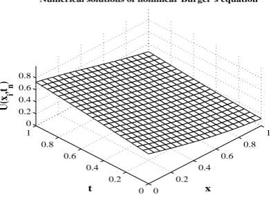
Table III presents the absolute error between exact and numerical solutions for problem B1 with ∆t= ∆x= 0.05 and the graphs of an exact and numerical solutions are shown in Fig. 4 and Fig. 5 respectively. Moreover, the graph of absolute errors is shown in Fig. 6. We can see that maximum of absolute error occurred at the middle spacexin each time step t.

TABLE III

ABSOLUTE ERROR BETWEEN EXACT AND NUMERICAL SOLUTIONS FOR

PROBLEMB1WITH∆t= ∆x= 0.05

t x

0.25 0.50 0.505 0.75

0 0.00 0.00 0.00 0.00

0.10 4.91×10−4 ₄_.₀₈_×₁₀−4 ₃_.₆₇_×₁₀−4 ₁_.₉₂_×₁₀−4

0.20 8.32×10−4 ₈_.₂₁_×₁₀−4 ₇_.₅₉_×₁₀−4 ₄_.₃₉_×₁₀−4

0.30 1.10×10−3 ₁_.₂₀_×₁₀−3 ₁_.₁₀_×₁₀−3 ₇_.₁₂_×₁₀−4

0.40 1.30×10−3 ₁_.₆₀_×₁₀−3 ₁_.₅₀_×₁₀−3 ₉_.₉₁_×₁₀−4

0.50 1.40×10−3 ₁_.₉₀_×₁₀−3 ₁_.₈₀_×₁₀−3 ₁_.₃₀_×₁₀−3

0.60 1.50×10−3 ₂_.₁₀_×₁₀−3 ₂_.₂₀_×₁₀−3 ₁_.₅₀_×₁₀−3

0.70 1.60×10−4 ₂_.₃₀_×₁₀−3 ₂_.₃₀_×₁₀−3 ₁_.₈₀_×₁₀−3

0.80 1.60×10−3 ₂_.₅₀_×₁₀−3 ₂_.₅₀_×₁₀−3 ₂_.₂₀_×₁₀−3

0.90 1.60×10−3 ₂_.₆₀_×₁₀−3 ₂_.₇₀_×₁₀−3 ₂_.₁₀_×₁₀−3

1.00 1.50×10−3 ₂_.₇₀_×₁₀−3 ₂_.₇₀_×₁₀−3 ₂_.₃₀_×₁₀−3

Table IV shows the maximum of absolute errors, we can see that the maximum of absolute error goes to zero as the mesh sizes∆xand∆t go to zero.

0 0.2

0.4 0.6

0.8 1

0 0.2 0.4 0.6 0.8 1 0 0.2 0.4 0.6 0.8

x Exact solutions of nonlinear Burger’s equation

t

U(x,t)

Fig. 4. The plot of exact solution for Problem B1 withc= 0,b= 1and µ0= 1/4.

0 0.2

0.4 0.6

0.8 1

0 0.2 0.4 0.6 0.8 1 0 0.2 0.4 0.6 0.8

x

Numerical solutions of nonlinear Burger’s equation

t

U(x

i

,t n

)

Fig. 5. The plot of numerical solutions for Problem B1 withc= 0,b= 1, µ0= 1/4,∆t= 0.05and∆x= 0.05.

0 0.2

0.4 0.6

0.8 1

0 0.2 0.4 0.6 0.8 1 0 1 2 3

x 10−3

x

Error between exact and numerical solutions of nonlinear Burger’s equation

t

[image:5.595.334.519.257.409.2]

Error

Fig. 6. The plot of absolute error between exact and numerical solutions for Problem B1.

TABLE IV

MAXIMUM OF ABSOLUTE ERRORS FORPROBLEMB1WITH∆x= ∆t

= 0.05,0.01,0.005,0.001

0.05 0.05 1.855×10−3

0.01 0.01 3.794×10−4

0.005 0.005 1.902×10−4

0.001 0.001 3.811×10−5

Case B2: Nonlinear modified Burger’s equation with 0≤µ1≤1.

We consider a modified Burger’s equation (14) in the form,

ut+R(u)ux=S(u)uxx, (31)

whereR(u) =c+bu and S(u) =µ0+µ1u.

FTCS implicit scheme is used in numerical solution, we get un+1_i −un

i

∆t +R(u n i)

un+1_i+1 −un+1_i₋₁ 2∆x

−S(un_i)u n+1 i+1 −2u

n+1

i +u

n+1 i−1

(∆x)2 = 0. (32)

Where∆t=τ and∆x=h,we have

IAENG International Journal of Applied Mathematics, 48:1, IJAM_48_1_08

[image:5.595.343.515.502.572.2]

(6)

un+1_i −un

i +R(uni) τ 2h

(

un+1_i+1 −un+1_i₋₁)

−S(un_i)_hτ2

(

un+1_i+1 −2un+1_i +un+1_i₋₁)= 0

[

−R(un_i)τ 2h−S(u

n i)

τ h2

]

un+1_i₋₁ −

[

−1−2S(un_i)τ h2

]

un+1_i

+[R(un i)

τ 2h−S(u

n i)

τ h2

]

un+1_i+1 =un i,

or

aiun+1i−1 −biun+1i +ciun+1i+1 =u n

i, (33)

i= 2, ..., M −1, n= 1, ...,[T /τ]−1,

where

ai= −R(uni)2hτ −S(u n i)hτ2,

bi= −1−2S(uni)hτ2,

ci= R(uni)2hτ −S(u n

i)hτ2, i= 2, ..., M−1.

We can see that equation (33) is the system of tridiagonal matrix. Numerical solutions are obtained by the sweep method.

Problem B2 : Let us consider nonlinear modified Burger’s equation (34) for c= 0, b= 1, µ0= 1₄ and

0≤µ1≤1 presents in the form,

ut+uux=

(

1 4 +µ1u

)

uxx, 0≤x≤1, 0≤t≤10 (34)

With initial condition : u(x,0) = 1 1+e2x, and boundary conditions :

u(0, t) = 1

1 +e−t, u(1, t) = 1 1 +e2−t.

Grid system :

Dh={(xi, tn)|xi= (i−1)∆x, tn= (n−1)∆t),

i= 1,2, ..., M, n= 1,2, ..., T}.

By FTCS implicit scheme, we have un+1_i −un

i

∆t +R(u n i)

un+1_i+1 −un+1_i₋₁ 2∆x

−S(un_i)u n+1 i+1 −2u

n+1

i +u

n+1 i−1

(∆x)2 = 0 (35)

u0i = 1 1 +e2xi,

un₁ = 1

1 +e−tn, u n

M =

1 1 +e2−tn.

Numerical solutions of a nonlinear modified Burger’s equa-tion (34) at fixed µ1 = 0.5 with vary time 0 ≤ t ≤ 10 are presented in Table V. We found that the numerical solutions will be increased and converge to 1.00 whereas time increases. In the case of fixed time, t = 5 and vary 0 ≤ µ1 ≤ 1 are shown in Fig. 7, we can see that the numerical solutions will be slightly decreased when µ1 increased. The graphs of numerical solutions of nonlinear modified Burger’s equation for µ1 = 0, 0.1, 0.5, 1.0 are shown in Fig. 8 - Fig. 11.

TABLE V

NUMERICAL SOLUTIONS OF NONLINEAR MODIFIEDBURGER’S EQUATION(34)AT FIXEDµ1= 0.5AND0≤t≤10

x= 0.00 x= 0.25 x= 0.50 x= 1.00

t= 0 0.500000 0.377540 0.268941 0.119202

t= 2 0.880797 0.800901 0.708335 0.500000

t= 5 0.999331 0.985310 0.975615 0.952574

t= 10 0.999954 0.999897 0.999827 0.999664

0 0.2 0.4 0.6 0.8 1

0.95 0.955 0.96 0.965 0.97 0.975 0.98 0.985 0.99 0.995 1

Numerical solutions of Modified Burgers equation at t=5

x

Numerical solutions

µ 1=0.0 µ

1=0.1 µ

[image:6.595.46.289.301.620.2]

1=0.5 µ₁=1.0

Fig. 7. The plot of numerical solutions of a nonlinear modified Burger’s equation (34) with t=5.

0 0.2

0.4 0.6

0.8 1

0 2 4 6 8 10

0 0.2 0.4 0.6 0.8 1

x

Numerical solutions of Modified Burger’s equation with µ₁ =0

t

U(x

i

,t n

)

Fig. 8. The plot of numerical solutions of a nonlinear modified Burger’s equation (34) atµ1= 0.

Case B3 : Nonlinear modified Burger’s equation for stationary solution withµ1= 0.

We consider a modified Burger’s equation (14) in the form,

ut+R(u)ux=S(u)uxx, (36)

whereR(u) =c+bu and S(u) =µ0+µ1u.

In casec= 1₂, b=−1 andµ0=14 andµ1= 0. We have,

ut+ ( 1

2 −u)ux= 1

4uxx, (37)

IAENG International Journal of Applied Mathematics, 48:1, IJAM_48_1_08

[image:6.595.315.523.408.556.2]

(7)

0 0.2

0.4 0.6

0.8 1

0 2 4 6 8 10

0 0.2 0.4 0.6 0.8 1

x Numerical solutions of Modified Burger’s equation with µ

1 =0.1

t

U(x

i

,t n

)

Fig. 9. The plot of numerical solutions of a nonlinear modified Burger’s equation (34) atµ1= 0.1.

0 0.2

0.4 0.6

0.8 1

0 2 4 6 8 10

0 0.2 0.4 0.6 0.8 1

1 =0.5

t

U(x

i

,t n

[image:7.595.65.262.56.204.2]

)

0 0.2

0.4 0.6

0.8 1

0 2 4 6 8 10

0 0.2 0.4 0.6 0.8 1

1 =1.0

t

U(x

i

,t n

[image:7.595.301.548.110.275.2]

)

un+1_i −un i

∆t +R(u n i)

un+1_i+1 −un+1_i₋₁

2∆x

−S(un_i)u n+1 i+1 −2u

n+1

i +u

n+1 i₋1

(∆x)2 = 0 (38)

Problem B3: Let us consider a nonlinear modified Burger’s equation (39)

ut+ ( 1

2 −u)ux= 1

4uxx, 0≤x≤10, 0≤t≤1. (39)

With initial condition : u(x,0) = 1₂(1 +tanh(x−5)), and boundary conditions : u(0, t) = 0 ,u(1, t) = 1.

Grid system :

Dh={(xi, tn)|xi= (i−1)∆x, tn = (n−1)∆t)},

i= 1,2, ..., M, n= 1,2, ..., T}.

By FTCS implicit scheme, we get un+1_i −un

i

∆t +R(u n i)

un+1_i+1 −un+1_i₋₁ 2∆x

−S(un_i)u n+1 i+1 −2u

n+1

i +u

n+1 i₋1

(∆x)2 = 0. (40)

u0_i = 1

2(1 +tanh(xi−5)),

un₁ = 0, un_M = 1.

The stationary solution of (39) with initial and boundary conditions has

u= 1

2(1 +tanh(x−5)).

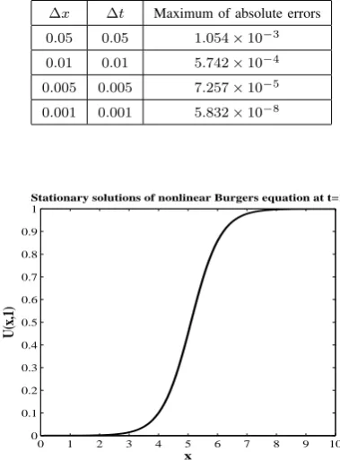
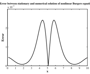
The graph of a stationary solution and absolute error of problem B3 at t = 1 are shown in Fig. 12, Fig. 13, Fig. 14 respectively.

TABLE VI

MAXIMUM OF ABSOLUTE ERRORS FORPROBLEMB3WITH ∆x= ∆t= 0.05,0.01,0.005,0.001ATt= 1

0.05 0.05 1.054×10−3

0.01 0.01 5.742×10−4 0.005 0.005 7.257×10−5

0.001 0.001 5.832×10−8

0 1 2 3 4 5 6 7 8 9 10

0 0.1 0.2 0.3 0.4 0.5 0.6 0.7 0.8 0.9 1

Stationary solutions of nonlinear Burgers equation at t=1

x

U(x,1)

Fig. 12. The plot of stationary solutions for Problem B3 withc=1 2,b= −1andµ0= 1/4 at t= 1.

Table VI shows the maximum of absolute errors, we can see that the maximum of absolute error goes to zero as the grid sizes∆xand∆tgo to zero.

IAENG International Journal of Applied Mathematics, 48:1, IJAM_48_1_08

[image:7.595.64.261.252.399.2] [image:7.595.325.515.445.702.2]

(8)

0 1 2 3 4 5 6 7 8 9 10 0

0.1 0.2 0.3 0.4 0.5 0.6 0.7 0.8 0.9 1

Numerical solutions of nonlinear Burgers equation at t=1

x

U(x

i

[image:8.595.64.263.53.209.2]

,1)

Fig. 13. The plot of numerical solution for Problem B3 withc= 1₂, b=−1, µ0= 1/4,∆t= 0.01and∆x= 0.01at t= 1.

0 1 2 3 4 5 6 7 8 9 10

0 1 2

x 10−4

x

Error

Error between stationary and numerical solution of nonlinear Burgers equation

Fig. 14. The plot of absolute error between stationary and numerical solutions for Problem B3 att= 1

IV. CONCLUSION

In this work, we have investigated the modified Burger’s equation in the form,

ut+ (c+bu)ux= (µ0+µ1u)uxx, (41)

where the parametersc,b,µ0andµ1 are given. An example of the linear Burger’ s equation (21) and the solutions were computed using the MATLAB program. We have found that the numerical solutions in the FTCS implicit scheme con-verge to related exact solutions is agreed with the theoretical convergence results.

Three cases of the numerical solutions for the nonlin-ear Burger’s equation were obtained by the FTCS implicit scheme as follows.

Case B1 : Nonlinear modified Burger’s equation in conservative form with

c= 0, b= 1, µ0= 1

4 andµ1= 0.

In the case, we have found that the numerical solutions obtained by the FTCS implicit scheme converge to the exact solution and the maximum of absolute error tends to zero when the grid sizes ∆xand∆t close to zero.

In the case, we have fixed time and varied the values of µ1 in 0 ≤ µ1 ≤1. The results showed that the numerical solutions are slightly decreased whenµ1is increasing. More-over, whenµ1is fixed, we found that the numerical solutions are increased and they are converged to1.00for all x as t is increasing.

Case B3 : Nonlinear modified Burger’s equation for stationary solution with

c=1

2, b=−1, µ0= 1

4 andµ1= 0.

In this case, we obtained the numerical solutions by the FTCS implicit scheme. All solutions are converged to the stationary exact solution.

ACKNOWLEDGMENT

I would like to express my sincere thanks to the De-partment of Mathematics, King Mongkut’s University of Technology North Bangkok (KMUTNB) for supporting us during this research.

REFERENCES

[1] Sebastien Blandin, Xavier Litrico and Alexandre Bayen, “Boundary stabilization of the inviscid Burgers equation using a Lyapunov method,”

49th_{IEEE Conference on Decision and Control}_{, pp. 1705-1712, 2010.} [2] Guo-cheng Wu, “Lie group classifications and exact solutions for

time-fractional Burgers equation,” pp. 1-9, 2010.

[3] Kanti Pandey and Lajja Verma, “A Note Crank-Nicolson Scheme for Burgers Equation,”Applied Mathematics, pp. 883-889, 2011. [4] Ram jiwari, “A Haar wavelet quasilinearization approach for numerical

simulation of Burgers equation,” Computer Physics Communications, vol. 183, pp. 2413-2423, 2012.

[5] Bruno Lombard, Denis Matignon and Yann Le Gorrec, “A fractional Burgers equation arising in nonlinear acoustics: theory and numeric,”

9th_{IFAC Symposium on Nonlinear Control Systems,}_{pp. 406-411, 2013.} [6] Ben Wongsaijai, Kanyuta Poochinapan, and Thongchai Disyadej, “A Compact Finite Difference Method for Solving the General Rosenau-RLW Equation,”IAENG International Journal of Applied Mathematics, vol. 44, no. 4, pp. 192-199, 2014.

[7] Dingwen Deng, and Tingting Pan, “A Fourth-order Singly Diagonally Implicit Runge-Kutta Method for Solving One-dimensional Burgers’ Equation,”IAENG International Journal of Applied Mathematics, vol. 45, no. 4, pp. 327-333, 2015.

[8] Ram Jiwari, “A hybrid numerical scheme for the numerical solution of the Burgers equation,”Computer Physics Communications, vol. 188, pp. 59-67, 2015.

[9] T. Zhanlav, O. Chuluunbaatar and V. Ulziibayar, “Higher-order accurate numerical solution of unsteady Burgers equation,”Applied Mathematics and Computational, vol. 250, pp. 701-707, 2015.

[10] Alaanttin Esen and orhun Tasbozan, “Numerical solution of time-fractional Burgers equation by Cubic B-spline finite elements,” Mediter-ranean journal of Mathematics, Birkhuser, pp. 1-13, 2015.

[11] A.H. Bhrawy, M.A. Zaky and D. Baleanu, “New numerical approx-imations for space-time fractional Burger’s equation VIA a Legendre spectral collocation method,”Romanian Reports in Physics, vol. 67, pp. 340-349, 2015.

[12] M. Seydaoglu, U. Erdogan and T.Ozis, “Numerical solution of Burger’s equation with high order splitting methods,”Journal of Computational and Applied Mathematics, vol. 291, pp. 410-421, 2016.

[13] John C. Tannehill, Dale A. Anderson and Richard H. Plrtcher. “Compu-tational fluid mechanics and heat transfer,”2nd_ed.,_{Taylor & Francis,} pp. 45-245, 1997.

[14] B. Jitsom, S. Sungnul and M. Punpocha, “Convergence of Numerical

IAENG International Journal of Applied Mathematics, 48:1, IJAM_48_1_08

[image:8.595.75.261.258.411.2]

(9)

Surattana Sungnulgraduated Ph.D. in Applied Mathematics, 2006, Surana-ree University of Technology, Thailand and is currently lecturer at the department of Mathematics, KMUTNB and a researcher in Centre of Excellence in Mathematics, THAILAND

Bubpha Jitsom graduated M.Sc. in Applied Mathematics, 2016, King Mongkut’s University of Technology North Bangkok, Thailand.

Mahosut Punpocha graduated Ph.D. in Mathematics, 2000, City University, UK and is currently lecturer at the department of Mathematics, KMUTNB.