Particle Swarm Optimization Feedforward Neural Network for Hourly Rainfall-runoff Modeling in Bedup Basin, Malaysia

Particle Swarm Optimization Feedforward Neural

Network for Hourly Rainfall-runoff Modeling in

Bedup Basin, Malaysia

Kuok King Kuok

, Sobri Harun

and Siti Mariyam Shamsuddin

Department of Hydraulics and Hydrology, Faculty of Civil Engineering, University Technology Malaysia, 81310 UTM, Johor, Malaysia

[email protected] 2

Department of Hydraulics and Hydrology, Faculty of Civil Engineering, University Technology Malaysia, 81310 UTM, Johor, Malaysia

[email protected] 3

Department of Computer Graphics and Multimedia, Faculty of Computer Science and Information System, University Technology Malaysia, 81310 UTM, Johor, Malaysia

[email protected]

Abstract

--

Index Term-- Modeling runoff, Backpropagation neural network (BPNN), Particle swarm optimization feedforward neural network (PS ONN), coefficient of correlation (R), Nash-S utcliffe coefficient (E2_).

1. INTRODUCTION

Various types of methods have been used in runoff estimation including conceptual and statistical models [1]. However, none of these methods can be considered as a single superior model [2]. Owing to the complexity of the hydrological process, the accurate runoff is difficult to be predicted using the linear recurrence relations or physically based watershed. The linear recurrence relation model does not attempt to take into account the nonlinear dynamic of hydrological process. The physically based watershed model also ignores the stochastic behavior underlying any hydrosystem. Besides, despite the application of deterministic models include all physical and chemical processes, the successful employment is restricted by a need for catchment-specific data and simplifications involved in solving the governing equations

[3]. The application of time series methods may be complicated by non-stationary and non-linearity in the data, requiring experience and expertise from the modeler [3]. Due to the difficulties of formulating reasonable nonlinear watershed model, artificial neural networks (ANNs) approach was applied for complex hydrologic modeling ([4], [5], [6], [7]).

In recent years, the application of ANNs in various aspects of hydrological modeling has undergone much investigation. The ability of ANNs to model non-linear relationship is appropriate to model the complex nature of hydrological systems. ANNs offer a relatively fast and flexible means of modeling. Besides, ANNs data are independent. ANNs do not impose functional relationship between independent and dependent variables. The functional relationship is determined by the data in the training process. The main advantage of ANNs is that a network with sufficient hidden units is able to approximate any continuous function to any degree of accuracy by performing efficient training ([8], [9]). When reviewed the application of ANNs in hydrology over the years, 90% of the researches are using multilayer feedforward neural network trained by standard backpropagation algorithmn (BPNN) [7]. Although BPNN proved to be efficient in some applications, its convergence rate is relatively slow and it often yields sub-optimal solutions ([10], [11], [12]).

BPNN learning basically is a hill climbing technique. Therefore, there is a risk of being trapped in local minima where every small change in synaptic weight increases the cost function. Sometime, the network is stuck where there exist another set of synaptic weight for which the cost function is smaller than the local minimum in the weight space. This made the BPNN undesirable to have the learning process terminate at a local minimum. Currently there are a few solutions proposed by Neural Network (NN) researcher to overcome this slow convergence rate problem.

Swarm Optimization (PSO) to form Particle Swarm Optimization Feedforward Neural Network (PSONN). The swarm is made up of particles, where each particle has a position and a velocity [13]. The function of PSO in NN is to get the best set of weight (or particle position) where several particles (problem solution) are trying to move or fly to get best solution. The application of PSONN in solving optimization problems is scarce. However, PSONN had been successfully applied in solving classification problems. PSONN was applied to solve the classification problems in medical domain [14] particularly in breast cancer and heart disease. PSO was applied to train NN for classifying Iris, Cancer, Wine, Diabetes, Hepatitis, Henan and Cubic data sets [15]. PSONN was proved to be more effective and efficient compared to Genetic Algorithm Backpropagation Neural Networks (GANN) for solving the classification problems using universal XOR, Cancer and Iris data set [16].

In this study, PSONN is employed to calibrate hourly rainfall-runoff relationship. The input data used are rainfall and rainfall-runoff data. The sensitivity of the PSONN performance to find the optimal architecture for achieving the best generalization errors possible was investigated using various data sets.

2. STUDY AREA

The selected study area is Sungai Bedup Basin, a sub-basin of Sadong Basin, Sarawak, Malaysia. This basin is located approximately 80km from Kuching City. For model calibration, data series used are only rainfall and observed runoff from year 1997 to year 1999.

The main boundary of Sadong Basin, rainfall and river stage gauging stations within Sadong Basin, are illustrated in Fig. 1. Bedup basin is located at upper stream of Batang Sadong where it is a non-tidal influence river basin. Fig. 2 shows the 5 rainfall gauging stations available in Sungai Bedup Basin, namely, Bukit Matuh (BM), Semuja Nonok (SN), Sungai Busit (SB), Sungai Merang (SM) and Sungai Teb (ST), and one river stage gauging station at Sungai Bedup located at the outlet of the basin.

Fig. 1. Location Map of Sadong Basin

Fig. 2. Bedup Basin Area with Stations

Bedup Basin covers a few villages, namely, Kampung Sungai Berok, Kampung Merjan and Kampung Longgo. The basin area is approximately about 47.5km2 and the elevation varies from 8m to 686m above mean sea level [17]. The vegetation cover is mainly of shrubs, low plant and forest. Sungai Bedup basin has a dendritic type channel system. The maximum stream length for the basin is approximately 10km, which is measured from the most remote area point of the stream to the basin outlet.

The input data used are daily rainfall data from the 5 rainfall stations. Observed hourly runoff and daily mean runoff data are converted from water level data through a rating curve given by Eq. (1) [18].

Q=9.19( H )1.9 (1) where Q is the discharge (m3/s) and H is the stage discharge (m). These observed runoff data were used to compare the model runoff.

3. PARTICLE SWARM OPTIM IZATION FEEDFORWARD

NEURAL NETWORK (PSONN)

3.1 Basic PSO Procedure

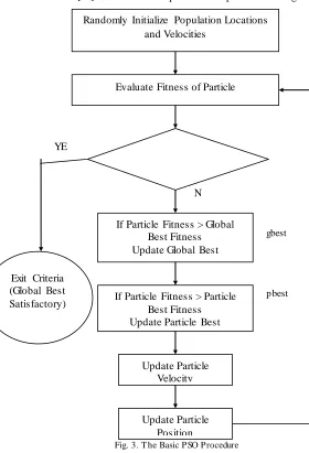
Particle swarm optimization (PSO), a new branch of the soft computing paradigms [19] called evolutionary algorithms (EA), was developed by Kennedy and Eberhart (1995). It is a group-based stochastic optimization technique for continuous nonlinear functions. It is also a simple concept adapted from nature decentralized and self-organized systems where all the particles move to get better results.

PSO is initialized with a group of random particles (solutions), which were assigned with random positions and velocities. The algorithm then searches for optima through a series of iterations where the particles are flown through the hyperspace searching for potential solutions. These particles learn over

time in response to their own experience and other p articles experience in their group [20].

Each particle keeps track of its best fitness position in hyperspace that has achieved so far [21]. This best position value is called personal best or “pbest”. The overall best value obtained by any particle so far in the population is called global best or “gbest”. During iteration, every particle is accelerated towards its own “pbest” as well as in the direction of the “gbest” position. This is achieved by calculating a new velocity term for each particle based on the distance from its “pbest” as well as its distance from the “gbest” position. These two “pbest” and “gbest” velocities are then randomly weighted to produce the new velocity value for this particle, which will affect the next position of the particle in next iteration [21]. The basic PSO procedure is presented in Fig. 3.

Meet Stopping Criteria

Fig. 3. T he Basic PSO Procedure

The advantage of the PSO over many of the other optimization algorithm is its relative simplicity [22]. The only two equations used in PSO are the movement equation (Eq. 2) and velocity update equation (Eq. 3) [23]. The movement equation provides for the actual movement of the particles using their specific vector velocity while the velocity updates equ ation provides for velocity vector adjustment given the two

competing forces (“gbest” and “pbest”). Besides, inertia weight () was introduced to improve the convergence rate of PSO algorithm [24].

t

V

on

prevLocati

on

presLocati







Vi =Vi-1 + c1*rand()*(pbest-presLocation)

+c2*rand()*(gbest-presLocation) (3)

where Vi is the current velocity,



t

interval over which the particle will move,  is the inertia weight, Vi-1 is the previous velocity, presLocation is the

present location of the particle, prevLocation is the previous location of the particle and rand() is a random number between (0, 1), c1 and c2 are the learning factors, stochastic

factors and acceleration constants for “gbest” and “pbest” respectively. Particles’ velocities are limited by a user-specified value, maximum velocity Vmax to prevent the

particles from flying too far from a target.

3.2 PSONN Algorithm

In this study, Particle Swarm Optimization (PSO) is applied to train feedforward neural network for enhancing the convergence rate and learning process. The basic element of NN is neuron. Each neuron is linked with its neighbors with an associated weight that represents information used by the net to solve a problem. The learning process involves finding a set of weights that minimizes the learning error.

The position of each particle in PSONN represents a set of weight for current iteration [25]. The dimension of each particle is the number of weights associated with the network. The learning error of this network is computed using Mean Squared Error (MSE). The particle will move within the weight space attempting to minimize learning error.

Fig. 4 shows the learning process of PSONN. The learning process of PSONN is initialized with a group of random particles (step 1), which were assigned with random PSO positions (weight and bias). The PSONN is trained using the initial particles position (step 2). Then, the feedforward NN in PSONN will produce the learning error (particle fitness) based on initial weight and bias (step 3). The learning error at current epoch will be reduced by changing the particles position, which will update the weight and bias of the network.

N

e

x

t

P

a

rt

ic

le

Exit Criteria (Global Best Satisfactory)

N 0

Randomly Initialize Population Locations and Velocities

Evaluate Fitness of Particle

If Particle Fitness > Global Best Fitness Update Global Best

If Particle Fitness > Particle Best Fitness Update Particle Best

Update Particle Velocity

Update Particle Position

gbest

pbest

Fig. 4. PSONN Learning P rocess

The “pbest” value (each particle’s lowest learning error so far) and “gbest” value (lowest learning error found in entire learning process so far) are applied to the velocity update equation (Eq. 2) to produce a value for positions adjustment to the best solution or targeted learning error (step 4). The new sets of positions (NN weight and bias) are produced by adding the calculated velocity value to the current position value using movement equation (Eq. 1). Then, the new sets of positions are used to produce new learning error in feedforward NN (step 5). This process is repeated until the stopping conditions either minimum learning error or maximum number of iteration are met (step 6). The optimization output, which is the solution for the optimizat ion problem, was based on gbest position value.

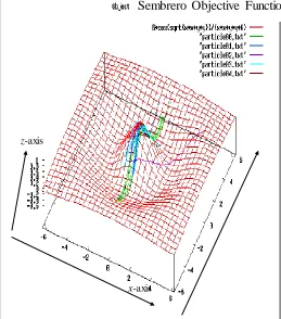
In this study, PSONN program has been developed based on PSO program for Sombrero function optimization. The particle position represents two-dimensional (2D) vector of x

and y values in Sombrero function. The objective is to reach the value of 1 based on value of x and y in Sombrero equation (Eq. 4) and the goal for the PSO is to maximize the function.

























6

*

*

*

*

cos

*

6

y

y

x

x

y

y

x

x

z

where x is value in x-axis, y is value in y-axis, z is value in z -axis.Fig. 5 shows that 5 particles move or fly to the solution in 2D problem to solve the Sombrero function. The fitness of the particle on the Sombrero is represented by z-axis.

Fig. 5. Particle Movement in Sombrero Function Optimization

4. MODEL DEVELOPM ENT

Various models were calibrated to determine to optimal configuration of PSONN models. PSONN architecture with well-selected parameter set can have good performance [26]. Hence, 7 parameters were investigate namely:

a) Acceleration constants for “gbest” (c1) b) Acceleration constants for “pbest” (c2) c) The time interval (Δt)

d) The number of particle (D).

e) Number of maximu m iteration (stopping condition) f) Number of hidden neurons

g) Length of training and testing data h) Number of antecedent hours.

Four basic parameters in PSO namely acceleration constants for “gbest” (c1), acceleration constants for “pbest” (c2), time interval (Δt), number of particles (D) are affecting the optimal configuration of PSONN [23]. Besides, other parameters including maximum iteration (stopping condition), number of hidden neurons in the hidden layer, length of input data and number of antecedent hours are also investigated for model calibration and optimization.

Meanwhile, parameters such as particle dimension also affect the optimization results. Number of dimension in PSONN is referring to number of weight and bias that is based on the dataset and PSONN architecture. PSONN dimension is calculated using Eq. 5.

Dimension =(input*hidden input hidden*output hidden)

+ hidden bias +output bias (5)

x-axis

y-axis

z-axis

TABLE I

Statistics for model comparison

5 models were developed to investigate the effect of antecedent hours to the configuration of PSONN. The input data of the models consists of antecedent rainfall, 1), P(t-2),…,P(t-n), antecedent runoff ,Q(t-1), Q(t-2),…,Q(t-n) and current rainfall, P(t). Where else, the output is the runoff at the current hour, Q(t). These 5 models are labeled as PSONNH1, PSONNH2, PSONNH3, PSONNH4 and PSONNH5.

4.1 Model PSONNH1

Q(t)=f[P(t),P(t-1),Q(t-1 (6)

4.2 Model PSONNH2

Q(t)=f[P(t),P(t-1),P(t-2),Q(t-1),Q(t-2)] (7)

4.3 Model PSONNH3

Q(t)=f[P(t),P(t-1),P(t-2),P(t-3),Q(t-1),Q(t-2),Q(t-3)] (8)

4.4 Model PSONNH4

Q(t)=f[P(t),P(t-1),P(t-2),P(t-3),P(t-4),Q(t-1),Q(t-2),Q(t-3),Q(t-4)] (9)

4.5 Model PSONNH5

Q(t)=f[P(t),P(t-1),P(t-2),P(t-3),P(t-4),P(t-5),Q(t-1),Q(t-2),Q(t-3),Q(t-4),Q(t-5)] (10) where t=time in hours, P=rainfall and Q=runoff. As time is one of the important factors in the model, the inputs shall be arranged in sequent.

The input data to PSONN need to be normalized as NN only work with data represented by numbers in the range between 0.001 and 0.999. The simplest normalization technique is dividing all data by the highest data value in that particular group (refer to Eq. 11). The output data need to be de-normalized to get the simulated runoff and compared with actual runoff.

x

x

y

max_



where y is the transform series and x is the original series of rainfall and runoff data.

The objective function used is Mean Squared Error (MSE). Optimization objective is important to ensure that Mean Squared Error (MSE) or learning error is getting lesser with the increase of number iterations. The PSONN performance is evaluated by Coefficient of correlation (R) and Nash -Sutcliffe coefficient (E2). R and E2 value of 1.0 implies a perfect fit and the formulas are presented in Table I.

5. LEARNING MECHANISM

Three layers PSONN was used in this study for model calibration. The number of input neurons depends on the model used (number of antecedent data) and there is only one neuron in the output layer. PSONN was trained and tested to find the best configuration using various dataset as shown below:

a) 1.6 to 2.2 of c1and c2 values.

b) Δt of 0.005, 0.010, 0.015, 0.020, 0.025 and 0.030 c) 17, 18, 19, 20, 21 and 22 numbers of particles. d) 75, 100, 125 and 150 number of hidden neurons in

hidden layer.

e) 400, 450, 500, 550 number of maximu m iteration. f) 3, 6, 9 and 12 months of training data and 1, 2, 3 and

4 months of testing data respectively. g) 1, 2, 3, 4 and 5 number of antecedent data.

6. RESULTS AND DISCUSSION 6.1 Number of Hidden Neurons

PSONN was investigated with 50, 75, 100 and 125 hidden neurons in the hidden layer. Table II presents that results obtained using various number of hidden neurons. Increasing number of hidden neuron from 50 to 100 increased the accuracy simulation results obtained. At 50 and 75 hidden neurons, the network may not have sufficient degrees of freedom to learn the process correctly. However, the performance of PSONNH4 starts to decrease at 125 hidden neurons. This is because at 125 hidden neurons, PSONNH4 takes a long time to get trained and may sometimes over fit the data. Thus, the optimal PSONNH4 model required 100 numbers of hidden neurons.

TABLE II

Performance Of PSONNH4 According T o Different Number Of Hidden Neurons Investigated. (PSONNH4 calibrated with c1and c2values of 2.0, 20

number of particles, Δt of 0.01, 9 months of training data, 3 months of testing data and 500 numbers of max iteration).

Different Hidden Neurons

Training Testing

R E2 R E2

50 0.847 0.8235 0.755 0.7713

75 0.882 0.8750 0.829 0.8871

100 0.975 0.9605 0.947 0.9461

125 0.912 0.8935 0.855 0.8966

6.2 Number of Maximum Iteration

PSONN is investigated with 400, 450, 500 and 550 numbers of maximum iteration. Table III compares the effect of various maximum iteration to PSONNH4. The performance of PSONNH4 improved with the increased of numbers of max iteration from 400 to 500 max iteration. At 400 and 450 maximum iterations, PSONNH4 is under trained and unable to approximate any continuous function to any degree of accuracy. In contrast, the PSONN performance decreased at 550 max iteration This may caused PSONN over trained and sometimes may over fit the data due to too many number of iterations are conducted. The best maximum iteration obtained

Coefficient Symbol Formula

Coefficient of Correlation R







Coefficient E2  









Note : obs = observed value, pred = predicted value, 

obs= mean

observed values, _pre_{d= mean predicted values and J = number of}

is 500 where it yields R=0.975 and E2=0.9605 for training data set and R=0.947 and E2=0.9461 for testing data set.

TABLE III

Performance Of PSONN According T o Different Maximum Iteration Investigated. (PSONNH4 calibrated with c1 and c2 values of 2.0, 20 number of

particles, Δt of 0.01, 9 months of training data, 3 months of testing data and 100 numbers of hidden neurons).

Different Maximum Iteration

Training Testing

R E2 R E2

400 0.836 0.8625 0.787 0.7936

450 0.883 0.8925 0.836 0.8647

500 0.975 0.9605 0.947 0.9461

550 0.935 0.9164 0.841 0.8692

6.3 Length of Training and Testing Data

The Performance of PSONN increased as the length of training increased from 3 to 9 months. The optimal length of 9 months training data is required to obtain an optimum result that yield R=0.975 and E2=0.9605 for training data set and R=0.947 and E2=0.9461 for testing data set. With more input data, PSONN will perform better as a more accurate determination of the synaptic weights is made by the PSONN. However, PSONN performance starts reducing at 12 months of training data. Table IV presented results of the four different length of training and testing data networks created, simulated with parameters of 100 hidden neurons, 500 maximu m iteration and 4 antecedent hours.

TABLE IV

Performance Of PSONN According T o Length Of Training And T esting Data Investigated. (PSONNH4 calibrated with c1 and c2 values of 2.0, 20 numbers

of particles, Δt of 0.01, 500 numbers of maximum iteration and 100 numbers of hidden neurons).

Length of Training

Data

Training Length of Testing

Data

Testing

R E2 R E2

3 months 0.968 0.9491 1 month 0.886 0.9270 6 months 0.970 0.9701 2 months 0.886 0.9339 9 months 0.975 0.9605 3 months 0.947 0.9461 12 months 0.874 0.7761 4 months 0.883 0.8233

6.4 Number of Antecedent Hours

The effect of number of antecedent days is to determine best time series to produce the best network. PSONNH4 performs the best with the highest coefficient of correlation and efficiency compared with other PSONN models as shown in Table V. The result showed that PSONNH4 is the optimal model for simulating hourly runoff in Bedup Basin.

Basically, the number of antecedent hours will determine the number of input neurons in input layer. For PSONNH1, PSONNH2 and PSONNH3, the network may not have sufficient degrees of freedom to learn the process correctly with little number of input neurons . In contrast, the number of input neuron is too high at PSONNH5. Hence, the network will take a long time to get trained as there are too many parameters to be estimated and may sometimes over fit the data.

TABLE V

Performance Of PSONN According T o Different Number Of Antecedent Hours Investigated. (PSONN calibrated with c1 and c2 values of 2.0, 20

number of particles, Δt of 0.01, 9 months of training data, 3 months of testing data , 500 numbers of maximum iteration and 100 numbers of hidden

neurons). Different

Antecedent Hours

Training Testing

R E2 R E2

PSONNH1 0.905 0.8994 0.820 0.8255

PSONNH2 0.975 0.9131 0.915 0.9242

PSONNH3 0.962 0.9670 0.898 0.9574

PSONNH4 0.975

0.9605 0.947 0.9461

PSONNH5 0.939 0.9238 0.840 0.8889

6.5 Different c1 and c2 Values

The acceleration constant c1 and c2 represent the stochastic acceleration that pulls each particle toward “pbest” and “gbest” position [21]. The c1constant affects the influence of

the global best solution over the particle, whereas the c2

constant affects how much influence of personal best solution has over the particle.

Reasonable results were obtained when PSONNH4 trained with acceleration constant, c1 and c2 values ranging from 1.6

to 2.2. The performance of PSONNH4 is improving as c1 and c2 values increased from 1.2 to 2.0. The reason is the particles

are attracted towards “pbest” and “gbest” with higher acceleration and abrupt movements when c1 and c2 values

increased from 1.2 to 2.0. Then, PSONNH4 performance decreased as c1 and c2 values decreased from 2.1 to 2.2. This

show PSONN is unable to converge with higher acceleration constant. Hence, the best c1 and c2 values required for optimal

configuration of PSONNH4 is 2.0 where R and E2 achieved 0.975 and 0.9605 for training, 0.947 and 0.9461 respectively for testing. The results for PSONNH4 trained with different c1

and c2values are tabulated in Table

VI.

TABLE VI

Performance Of PSONN According T o Different c1 and c2values.

(PSONNH4 calibrated with 20 numbers of particles, Δt of 0.01, 9 months of training data, 3 months of testing data, 500 numbers of maximum iteration

and 100 numbers of hidden neurons).

c

and

c

values

Training

Testing

R

E

R

E

1.6

0.928

0.8387

0.783

0.8085

1.7

0.960

0.9617

0.867

0.9189

1.8 0.952 0.9341 0.839 0.8864

1.9

0.971

0.9298

0.861

0.9147

2.0 0.975 0.9605

0.947

0.9461

2.1

0.966

0.9679

0.885

0.8947

2.2

0.965

0.9784

0.839

0.9008

6.6 Different Δt

solution space and higher Δt value performs lower granularity movement (greater distance achieved in less time).

The Performance of PSONNH4 increased as Δt increased from 0.005 to 0.01. PSONN is unable to converge at Δt of 0.005 due to the high granularity movement within the solution space. However, PSONNH4 performance is slightly decreased at Δt of 0.015. Then, PSONNH4 performance improved to R=0.951 and E2=0.9730 for training and R=0.830 and E2=0.8936 for testing at Δt of 0.020. PSONNH4 performance decreased again from Δt of 0.025 to 0.030. This is due to the low granularity movement within solution space. It was concluded the best Δt obtained in this study is 0.010 where R and E2 yield to 0.975 and 0.9605 respectively for training and 0.947 and 0.9461 respectively for testing. Table VII presents the performance of PSONNH4 when trained and tested with different Δt.

TABLE VII

Performance Of PSONN According T o Different Δt. (PSONN calibrated with

c1 and c2 values of 2.0, 20 number of particles, 9 months of training data, 3

months of testing data , 500 numbers of maximum iteration and 100 numbers of hidden neurons).

Δt values Training Testing

R E2 R E2

0.005 0.911 0.8527 0.758 0.8234

0.010 0.975 0.9605 0.947 0.9461

0.015 0.931 0.8267 0.763 0.8742

0.020 0.951 0.9730 0.830 0.8936

0.025 0.942 0.9675 0.877 0.8835

0.030 0.896 0.8807 0.704 0.8702

6.7 Different D

The number of particles in PSO determines the amount of space that is covered in the problem. The performance of PSONN increased with the increase of number of particles from 17 to 20. PSONN is unable to simulate well at 17, 18 and 19 numbers of particles because the space covered in the problem is not sufficient. Then, at 21 numbers of particles, the PSONN performance starts decreasing (refer to Table VIII) due to the space covered in solving the problem is too wide. The PSONNH4 performance is slightly improved with 22 numbers of particles. Generally, this study indicates that the best number of particles was found to be 20. The optimization period was getting longer with the increase of number of particles. This is because the more particles that are presented, the greater the amount of space that is covered in the problem.

TABLE VIII

Performance Of PSONN According T o Different Number Particles. (PSONN calibrated with c1 and c2 values of 2.0, Δt of 0.01, 9 months of training data, 3

months of testing data , 500 numbers of maximum iteration and 100 numbers of hidden neurons).

D Training Testing

R E2 R E2

17 0.967 0.9678 0.854 0.8920

18 0.908 0.9065 0.752 0.8079

19 0.938 0.9136 0.825 0.8738 20 0.975 0.9605 0.947 0.9461

21 0.955 0.9517 0.834 0.8704

22 0.968 0.9705 0.881 0.9018

6.8 Optimal Configuration of PSONN Network

The optimal configuration for PSONN network was found to be as follow:

a) Number of Hidden Neurons = 100 b) Number of Max Iteration = 500 c) Length of Training Data = 9 months

d) Number of antecedent data = 4 (PSONNH4) e) c1 and c2 values of 2.0

f) Time interval of 0.0100 g) 20 number of particles

6.9 Runoff Simulation with Lead-time

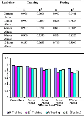
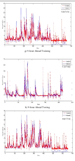
The optimal PSONN model determined above is will be used to generate hourly runoff with lead-time of 3, 6, 9 and 12-hour ahead. The results of this study are presented in Table IX, Fig. 6 and Fig. 7.

TABLE IX

Runoff Simulation Results at Different Lead-time using Optimal PSONN Model.

Lead-time Training Testing

R E2 R E2

Current hour

0.975 0.9605 0.947 0.9461

3-hour Ahead

0.957 0.9070 0.878 0.8836

6-hour Ahead

0.907 0.8211 0.853 0.8695

9-hour Ahead

0.900 0.7530 0.824 0.8525

12-hour Ahead

0.887 0.7633 0.740 0.8090

0 0.2 0.4 0.6 0.8 1 1.2

Current hour 3-hour

Ahead

6-hour Ahead

9-hour Ahead

12-hour Ahead

R a n d E V a lu e s

Different Lead Time

R Training E Training R Testing E (Testing)

2 2

2

a) Current Hour for T raining

b) Current Hour for T esting

c) 3-hour Ahead T raining

d) 3-hour Ahead T esting

e) 6-hour Ahead T raining

g) 9-hour Ahead T raining

h) 9-hour Ahead T esting

i) 12-hour Ahead T raining

j) 12-hour Ahead T esting

Fig. 7. Performance of PSONN for Runoff Simulation at Different lead-time.

Table IX and Fig. 6 show that the performance for PSONN is decreased with the increase of lead-time. For training dataset, R values produced by PSONNH4 with 3, 6, 9 and 12-hour ahead runoff forecast decreased from 0.957, 0.907, 0.900 to 0.887. Meanwhile, E2 decreased from 0.9070, 0.8211, 0.7530 to 0.7633 too. Similarly for testing dataset, R values obtained by PSONNH4 for 3, 6, 9 and 12-hour ahead runoff forecast are decreasing from 0.878, 0.853, 0.824 to 0.740. Average E2 also decreased from 0.8836, 0.8695, 0.8525 to 0.8090 with the increased of lead time from 3, 6, 9 and 12-hour ahead runoff forecast. It was observed that the hourly simulated obtained through PSONN is successful in approaching the maximum discharges but less successful in calculating the low discharges.

7.0 CONCLUSION

In this study, PSONN is successfully developed for hourly runoff simulation for Bedup Basin. The result show that this PSO based algorithm can train the NN as other existing techniques. The best PSONN for hourly runoff prediction is model PSONNH4 by yielding R=0.975 and E2=0.9605 for training dataset and R=0.947 and E2=0.9461 for testing dataset. Besides, the best configuration for modeling hourly rainfall-runoff relationship is using 100 numbers of hidden neuron, 500 numbers of maximum iteration, 9 months of input data for training and 3 months of testing data, 4 antecedent hours, c1 and c2 of 2.0, 20 numbers of particles and Δt of

0.010. Meanwhile, the optimal model of PSONN is also able to predict the runoff accurately at the lead-time of 3, 6, 9 and 12-hour ahead.

particles position are updated using movement equation (Eq. 2) and velocity update equation (Eq. 3), which search for “pbest” and “gbest” values. This will avoid the weight and biases being trapped in local minima. Besides, it was also found that input data including current rainfall, antecedent rainfall and antecedent runoff are sufficient enough for PSONN to predict current runoff accurately.

REFERENCES

[1] World Meteorological Organisation (WMO). (1994). “Guide for Hydrological Practices”. Geneva, Switzerland.

[2] Shamseldin, A.Y. (1997). “ Application of a Neural Network T echnique to Rainfall-runoff Modelling”. Journal of .Hydrology. 199, 272-294.

[3] Imrie, C.E., Durucan, S. and Korre, A. (2000). “ River Flow Prediction Using Artificial Neural Networks: Generalization Beyond the Calibration Range”. Journal of Hydrology, 233: 138-153, 2000.

[4] Saad, M., Bigras, P., T urgeon, A., Duquette, R. (1996). “ Fuzzy Learning Decomposition for the Scheduling of Hydroelectric Power Systems”. Water Resour. Res. 32(1), 179-186. [5] Clair, T .A. and Ehrman, J.M. (1998).” Using Neural Network to

assess the Influence of Changing Seasonal Climates in Modifying Discharge, Dissolved Organic Carbon, and Nitrogen Export in Eastern Canadian Rivers”. Water Resour. Res. 34(3), 447-455. [6] Jain, S.K., and Chalisgaonkar, C. (2000). “ Setting Up Stage-Discharge Relations Using ANN”, Journal of Hydrologic Engineering, 5(4), 424-433, 2000.

[7] Coulibaly, P., Anctil, F., Bobee, B., (2000). “ A Recurrent Neural Networks Approach Using Indices of Low-frequency Climatic Variability to Forecast Regional Annual Runoff”. Neural Networks

2(6), 121-135

[8] Cybenko, G. (1989). “Approxim ation By Superposition of a Sigm oidal Function, Math. Control Signals Syst”. 2, 303-314.

[9] Hornik, K., Stinchcombe, M., White, H. (1989). “ Multilayer Feedforward Networks are Universal Approximators”. Neural Networks 2(5), 359-366.

[10] Baldi, P., Hornik, K. (1989). “ Neural Network and Principal Component Analysis: Learning from Examples Without Local Minima”. Neural Networks 2(1), 53-58.

[11] Mulenbein, H. (1990). “ Limitations of Multilayer Perceptron Networks-Steps T owards Genetic Neural Networks”. Parallel Com puting 14, 249-260.

[12] Sima, S. (1996). “ Backpropagation is Not Efficient ”. Neural Networks 9(6), 1017-1023.

[13] Van den Bergh, F. (1999). “ Particle Swarm Weight Initialization In Multi-Layer Perceptron Artificial Neural Networks”. ICAI. Durban, South Africa.

[14] Zhang, C., Shao, H. and Li, Y. (2000). “ Particle Swarm Optimization for Evolving Artificial Neural Network ”. IEEE: 2487-2490.

[15] Van den Bergh, (2001). “An analysis of Particle Swarm Optim izers”. Ph.D dissertation,University of P retoria, South

Africa.

[16] Haza, N. (2006). “Particle Swarm Optimization for neural network learning enhancement”. Msc. T hesis, University T echnology of

Malaysia.

[17] JUPEM (1975). “National Mapping Malaysia”. Scale 1:50,000

[18] DID (2004). “Hydrological Year Book Year 2004”. Department of Drainage and Irrigation Sarawak, Malaysia.

[19] J. Kennedy and R.C. Eberhart (1995). “ Particle Swarm Optimization”. In Proceedings of the IEEE International Joint Conference on Neural Networks, pages 1942–1948. IEEE Press. [20] Ferguson, D. (2004). “Particle Swarm”. University of Victoria,

Canada.

[21] R. Eberhart, Y. Shi. (2001). “ Particle swarm optimization: developments, applications and resources”. IEEE Int. Conf. on Evolutionary Com putation, 2001: 81-86.

[22] Van den Bergh, F. and Engelbrecht, A. P. (2000). “ Cooperative Learning in Neural Networks using Particle Swarm Optimizers”.

South African Com puter Journal. (26):84-90.

[23] Jones M.T (2005). “AI Application Program m ing”. 2nd Ed. Hingham, Massachusetts:

[24] Y. Shi and R.C. Eberhart (1998). “ A Modified Particle Swarm Optimizer”. Proceedings of the 105 IEEE Congress on Evolutionary Com putation, p. 69–73, May 1998.

[25] Al-kazemi, B. and Mohan, C.K. (2002). “ T raining Feedforward Neural Network Using Multi-phase Particle Swarm Optimization”.

Proceeding of the 9th _{International Conference on Neural}

Inform ation Processing. New York.