www.j-sens-sens-syst.net/4/97/2015/ doi:10.5194/jsss-4-97-2015
© Author(s) 2015. CC Attribution 3.0 License.
A systematic MEMS sensor calibration framework
A. Dickow and G. Feiertag
Munich University of Applied Sciences, Munich, Germany
Correspondence to: A. Dickow ([email protected])
Received: 28 October 2014 – Revised: 31 December 2014 – Accepted: 13 January 2015 – Published: 27 February 2015
Abstract. In this paper we present a systematic method to determine sets of close to optimal sensor calibration points for a polynomial approximation.
For each set of calibration points a polynomial is used to fit the nonlinear sensor response to the calibration reference. The polynomial parameters are calculated using ordinary least square fit. To determine the quality of each calibration, reference sensor data is measured at discrete test conditions. As an error indicator for the quality of a calibration the root mean square deviation between the calibration polynomial and the reference measurement is calculated. The calibration polynomials and the error indicators are calculated for all possible calibration point sets. To find close to optimal calibration point sets, the worst 99 % of the calibration options are dismissed. This results in a multi-dimensional probability distribution of the probably best calibration point sets. In an experiment, barometric MEMS (micro-electromechanical systems) pressure sensors are calibrated using the proposed calibration method at several temperatures and pressures. The framework is applied to a batch of six of each of the following sensor types: Bosch BMP085, Bosch BMP180, and EPCOS T5400. Results indicate which set of calibration points should be chosen to achieve good calibration results.
1 Introduction
MEMS (micro-electromechanical systems) sensors are cali-brated at one or several points at the end of the production process in order to fulfill the product specifications. Various techniques can be applied to compensate sensor nonlineari-ties (see Brignell, 1987). In many cases (e.g., humidity sors, gyroscopes, pressure sensors, barometric pressure sen-sors) calibration relies on a polynomial for fitting the raw sensor data readout to reference signals (van der Horn and Hujising, 1997; Lyahou et al., 1996; Cerry et al., 1990; Bolk, 1985). Usually production issues limit the number of cali-bration points available for calibrating sensors against a ref-erence. An adequate choice of calibration points can reduce the number of calibration points and thus sensor calibration time and cost (see Dickow and Feiertag, 2014). As far as we know, no systematic technique for MEMS sensor calibration has been published, including both optimal calibration point selection and calibration using as few points as possible. In this paper a polynomial approach for MEMS sensor calibra-tion with only a few calibracalibra-tion points is proposed. An alge-braic framework is used to determine all possible calibration
point combinations. In an experiment, the proposed method is applied to barometric MEMS pressure sensors. Recom-mendations are made for an optimal choice of calibration points. The paper is structured as follows: Sect. 2 introduces the concept of polynomial calibration with parameter extrap-olation; in Sect. 3 a combinatorial framework is proposed for the selection of calibration point sets; in Sect. 4 the proposed framework is applied to barometric MEMS pressure sensors; and in Sect. 5 the results are discussed in a conclusion.
2 Calibration using polynomial regression
and Filzmoser, 2009. As multiple OLS is a linear regression method, calibration functions have to be linear in their pa-rameters. In this paper a multivariable polynomial is chosen as the calibration function to linearize the sensor behavior over specification. The polynomial function is capable of lin-earizing continuous, differentiable sensor readouts to a given specification. In some cases, polynomial functions of very high order are needed to reach the desired calibration accu-racy. Then, it is useful to switch to other functions, reach-ing accuracy goals with fewer parameters, or even switch to other regression methods, e.g., support vector regression (see Smola and Scholkopf, 2004).
2.1 Linear regression model for polynomial calibration
A calibration function gives the sensor output signal as a function of the sensor’s raw values. Multiple regression cal-ibration is used to generate an appropriate calcal-ibration func-tion for given reference values. The OLS calibrafunc-tion method is an integral part of research and production in many fields of applications (shown in Eriksson et al., 2006). A linear re-gression model forN observations can be expressed as
y=Xβ+ε, (1)
wherey is denoted as dependent variable (set of reference values measured at the calibration points), X is a matrix of independent variables (functions of sensor raw values at the calibration points),βis the calibration parameter vector and
εis the error term vector, describing the calibration errors at the distinct calibration points.
In matrix notation, the calibration problem transforms to
y1 . . . yN =
1 x11 . . . x1M . . . . . . . .. .. . 1 x1N . . . xN M
β0 . . . βM + ε1 . . . εN
, (2)
whereM=N−1 and rank(X)=N. Ncalibration points are required to calculate a unique solution for the calibration pa-rametersβ. Each single row ofXdescribes an independent variable vector of the calibration function used. An indepen-dent variable vector
1, xij, . . ., xiM describes transformed
raw sensor readouts at specific reference sensor readout yi.
When calibration uses a polynomial function with a single raw sensor readout signal,M=N−1 is also the polynomial orderK; so that
yk,poly =β0+β1xraw,k+β2xraw,k2 +. . .+βKxraw,kK
=
K
X
i=0
βixraw,ki =β0+ M
X
i=1
βixk,i (3)
describes the polynomial approximation of yk, where k∈
(1, . . ., N ). IfM < N−1, the OLS fit produces an errorεk.
When havingp raw sensor readout signals, the polynomial
approximation expands to
yk,poly = p Y j=1 Kj X i=0
βj,ixraw,j,ki
=β0+ M
X
i=1
βixk,i, (4)
needing
N=M+1=
p
Y
j=1
Kj+1
(5)
calibration points to calculate a unique solution to the multi-ple sensor signal calibration problem. The parameterKj, j∈
1, . . ., p
describes the polynomial order for each raw sensor signal used for calibration.
For example, MEMS pressure sensors with raw tempera-turexraw,T and raw pressure readoutxraw,P are usually
cali-brated with a polynomial of order 2 in temperature and order 1 in pressure:
ypoly =
β1,0+β1,1xraw,T+β1,2xraw,T2
β2,0+β2,1xraw,P
=β0+β1xraw,T+β2xraw,T2 +β3xraw,P+β4xraw,Pxraw,T
+β5xraw,Pxraw,T2 . (6)
In this case, N=(2+1)(1+1), six calibration points are required to determine all calibration parametersβi, i∈
(0, . . .,5).
2.2 Calibration criteria and option selection
In the following ki denotes a set of calibration points. For
the example from Eq. (6), each ki contains three
tempera-ture points (T1,T2,T3) and two pressure points (P1,P2) coupled in a row, leading to
ki=
(P1, T1)
(P1, T2)
(P1, T3)
(P2, T1)
(P2, T2)
(P2, T3)
. (7)
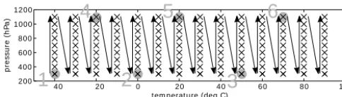
To decide which sets of calibration points give the best sensor accuracy a reference data set is necessary. This refer-ence data is measured at discrete values within the measure-ment range of the sensor. In the following we assume that all calibration points match the discrete values of the refer-ence data. This leads to a finite number of possible sets of calibration point combinations [k1, . . .,kL].In Fig. 1 this is
shown for the example given above. The reference data was measured for all points denoted with an “X”, the group of six grey circles is one set of calibration points.
For eachki, the OLS regression is performed using the
40 20 0 20 40 60 80 100 t em perat ure (deg C)
200 400 600 800 1000 1200
p
res
s
u
re
(h
P
a
)
1
2
3
4
5
6
Figure 1.Six selected calibration points for digital barometric pres-sure sensors, chosen from a reference data set (marked with ×); recorded data is in ascending order to avoid temperature hysteresis effects.
evaluate the calibration quality, the identified parameters are inserted intoypolyand used to calculate the calibration error
over the sensor working range. As calibration error indicator, the calibration root mean squared error (rms error),
e=
v u u t
1 R−1
R X
j=0
yj,poly(βj,xj,raw,1, . . .,xj,raw,p)−yj,ref
2, (8)
is calculated from the reference datayrefand the polynomial approximationypoly, whereRis the number of reference data points. N < Rdescribes the case, when more than one cal-ibration option is available. In this case the calcal-ibration task has
Ocal=
Rj
Kj+1
K
(9)
possible calibration options. For a multidimensional calibra-tion problem
Ocal=
p
Y
j=1
Rj
Kj+1
Kj
(10)
calibration options are possible, when the sensor is influ-enced bypsignals/factors. From all calibration options,
C=k1, k2, . . ., kOcal
,C∈RN xOcal, (11)
those are seen as optimal calibration options0, where
0=hek1, . . ., ekOcal
i
. (12)
2.3 Statistical evaluation
For a batch ofIsensors, with evaluated rms errors at C, there are
O0= {01, . . ., 0I} (13)
optimal calibration options. It can happen that some optimal calibration options are identical. If the batch of sensors is representative for a specific sensor type, the most common optimal calibration option should be preferred. However as sensors are influenced by multiple parameters, it is not very
likely to find sensors having exactly the same calibration rec-ommendation.
To retrieve more information about fields of attraction for best calibration options in a multidimensional optimization problem, a selection criteria weaker than Eq. (12) is pro-posed. The criteria
099⊂
h
ek1, . . ., ekOcal
i
(14)
dismisses those 99 % calibration options, which have the highest rms errors according to Eq. (8). The099 criteria is
applied to each sensor of a batch. This results in a calibration recommendation for an investigated sensor type
0r99=099,1, . . ., 099,I, (15)
which will be used in the following as a multidimensional indicator for close to optimal calibration points.
3 Software implementation
The proposed sensor calibration approach was implemented in a framework, written in Python language, to investigate commercial MEMS sensors with digital data readout. It uses the Fortran package LAPACK (Linear Algebra PACKage) to solve linear equations using LU (lower, upper) decom-position (Strang, 1980) with partial pivoting and row inter-change. A typical calibration workflow is depicted in Ta-ble 1. Four steps are needed to retrieve meaningful statisti-cal data out of given digital raw sensor readout and reference values: data processing, calibration, comparison and statisti-cal evaluation. If the number of required statisti-calibration points N is much smaller than the amount of available reference points for calibrationRor more than two independent sensor readoutspare used for calibration, the amount of OLS calls can get too high for desktop computers to solve within a rea-sonable time. In consequence, the framework should only be used for low- to medium-order polynomials, having only a few independent readout signals used for calibration.
4 Application example – barometric MEMS pressure
sensors
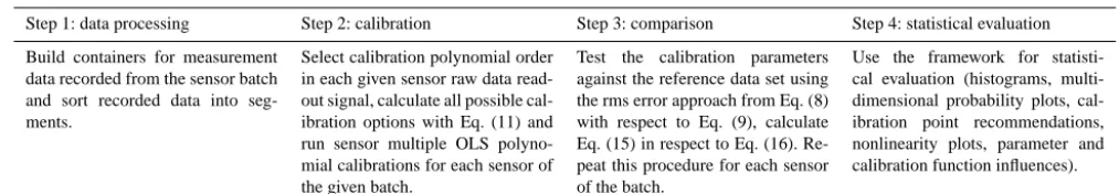
multipara-Table 1. A typical calibration workflow using the proposed framework; data processing, calibration and evaluation are implemented in independent modules.
Step 1: data processing Step 2: calibration Step 3: comparison Step 4: statistical evaluation
Build containers for measurement data recorded from the sensor batch and sort recorded data into seg-ments.
Select calibration polynomial order in each given sensor raw data read-out signal, calculate all possible cal-ibration options with Eq. (11) and run sensor multiple OLS polyno-mial calibrations for each sensor of the given batch.
Test the calibration parameters against the reference data set using the rms error approach from Eq. (8) with respect to Eq. (9), calculate Eq. (15) in respect to Eq. (16). Re-peat this procedure for each sensor of the batch.
Use the framework for statisti-cal evaluation (histograms, multi-dimensional probability plots, cal-ibration point recommendations, nonlinearity plots, parameter and calibration function influences).
metrical second-order calibration polynomial,
yBaro=β0+β1xraw,t+β2xraw,t2 +β3xraw,p
+β4xraw,txraw,p+β5xraw,t2 xraw,p, (16)
using the sensor’s raw temperature readoutxraw,t and a raw
pressure readoutxraw,p.
4.1 Calibration setup
The test equipment uses a pressurized climate chamber, a General Electric PACE 5000 pressure controller as pressure calibration reference and a combination of Peltier elements and a type K thermocouple for reference temperature con-trol, attached close to the sensor site. Data is recorded using a National Instruments USB-8451 I2C device, connected to the digital barometric MEMS pressure sensors, soldered on to a printed circuit board.
4.2 Calibration task
For all further investigations, it is assumed that the sensors deliver reproducible results. As barometric MEMS pressure sensors suffer from temperature hysteresis (see Waber et al., 2013), data was recorded in ascending temperature order to minimize the hysteresis effect.
Sensors used in the experiment have a measurement range from −40 to 90◦C and from 300 to 1100 hPa. To test the calculated sensor calibration, discrete points at [−40,−30, . . . , 90◦C] are chosen as test temperature points and [300, 400, . . . , 1100 hPa] are chosen as test pressure points. Within the measurement range, the sensor’s raw values, the refer-ence pressure and the referrefer-ence temperature are recorded in a sequence to avoid disturbances from temperature hystere-sis, as described in Fig. 1. At each point, the measurement device waits until stable pressure and temperature conditions are reached. Data recorded consists of time stamp, raw pres-sure, raw temperature, reference pressure and reference tem-perature. Six points are numerated and marked in grey. They exemplarily stand for a calibration point set, as presented in Eq. (7). In the following, this and all other possible calibra-tion opcalibra-tions will be evaluated to determine the best combina-tions possible.
4.3 Calibration point recommendation
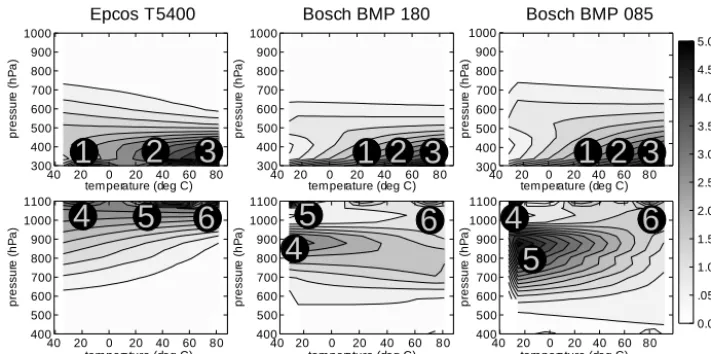
Data is recorded according to the description in Sect. 4.2. For the calibration polynomial from Eq. (16), the most likely best calibration point combinations were calculated using the procedure taken from Table 1. The experimental results are shown in a distribution landscape plot in Fig. 2. The plot ex-emplarily separates the first 3 calibration points (upper row in Fig. 2) from the calibration points 4–6 (second row in Fig. 2). This clustering into two distribution plots provides informa-tion about how to combine temperature points, when calibra-tion is restricted to only two possible pressure condicalibra-tions, as it can happen in industrial sensor production to save calibra-tion time. Figure 2 shows, that the investigated T5400 sensor should be calibrated at points at the borders of pressure range (300 and 1100 hPa), while the other sensor types investigated show a more heterogeneous calibration point recommenda-tion (300, 900 and 1100 hPa).
5 Other applications
40 20 0 20 40 60 80 300 400 500 600 700 800 900 1000 p re ssu re (hP a )
40 20 0 20 40 60 80 400 500 600 700 800 900 1000 1100 pr es s u re (hP a )
20 0 20 40 60 80 300 400 500 600 700 800 900 1000 p re ssu re (h P a )
20 0 20 40 60 80 400 500 600 700 800 900 1000 1100 p re ssu re (h P a )
20 0 20 40 60 80
p re ssu re (h P a )
40 20 0 20 40 60 80 400 500 600 700 800 900 1000 1100 p re ssu re (h P a ) 0.0 .05 1.0 1.5 2.0 2.5 3.0 3.5 4.0 4.5 5.0 300 400 500 600 700 800 900 1000
Epcos T5400 Bosch BMP 180 Bosch BMP 085
temperature (deg C) 40 40
40
temperature (deg C) temperature (deg C)
temperature (deg C) temperature (deg C) temperature (deg C)
rel a tiv e fre quenc y (%)
1
2
3
4
5
6
1 2 3
4
5
6
1 2 3
4
5
6
Figure 2.Recommended six calibration points for second order polynomial barometric pressure sensor calibration; frequency of the first three calibration points shown in the upper part; frequency of the last three calibration points shown in the lower part of the figure.
6 Conclusions
The proposed framework was used to calibrate barometric MEMS pressure sensors with six calibration points and a second-order calibration polynomial in temperature and first-order in pressure. For all sensors investigated, points selected at the upper and lower borders of temperature and pressure range increase the likelihood of appearing within the best 1 % of the calibration options. The proposed framework deter-mines all possible calibration options for a given set of sensor measurement data using a linear polynomial regression ap-proach and then applies the rms error over measured test con-ditions as calibration benchmark. The worst 99 % of the cal-ibrations are dismissed to show areas of attraction for good calibration options. For further research, calibration point ex-trapolation will be implemented to reduce the amount of cal-ibration points measured. This is used to achieve the sensor specification required by statistically estimating offset values for higher-order calibration polynomial parameters. Further calibration uncertainty considerations will be evaluated ac-cording to Waber et al. (2013), Heydorn and Anglov (2002) and Brüggemann and Wennrich (2002).
Acknowledgements. This work was supported by the Bavarian ministry of economic affairs within the research project MEMS-Baro.
Edited by: N.-T. Nguyen
Reviewed by: two anonymous referees
References
Aggarwal, P., Syed, Z., Niu, X., and El-Sheimy, N.: Cost-effective Testing and Calibration of Low Cost MEMS Sensors for Inte-grated Positioning, Navigation and Mapping Systems, XXIII FIG Congress, Munich, Germany, 8–13 October 2006.
Bolk, W. T.: A general digital linearising method for transducers, J. Phys. E: Sci. Instrum., 18, 61–64, 1985.
Bosch Sensortec: “BST-BMP085-DS000-03”, BMP 085 digital pressure sensor datasheet, Rev. 1.0, July 2008.
Bosch Sensortec: “BST-BMP180-DS000-09”, BMP 180 digital pressure sensor datasheet, Rev. 2.5, April 2013.
Brignell, J.: Digital compensation of sensors, J. Phys. E: Sci. In-strum., 20, 1097–1102, 1987.
Brüggemann, L. and Wennrich, R.: Evaluation of measurement un-certainty for analytical procedures using a linear calibration func-tion, Accred. Qual. Assur., 7, 269–273, 2002.
Cerry, S., Baer, W., Cowles, J., and Wise, K.: Digital compensation of high-performance silicon pressure transducers, Sensor. Actu-ators, A2I–A23, 70–72, 1990.
Dickow, A. and Feiertag, G.: A framework for calibration of baro-metric MEMS pressure sensors, Eurosensors conference 2014, Brescia, Italy, 7–10 September 2014.
EPCOS: “Saw Components Application Note T5400”, T5400 digi-tal pressure sensor application note, Rev 1.3.A1, February 2013. Eriksson, L., Johansson, E., Kettaneh-Wold. N., Trygg, J., Wik-ström, C., and Wold, S.: Multi- and Megavariate Data Analysis – Part 1 Basic Principles and Applications, 2nd Edn., Umetrics AB, Umea, Sweden, p. 127, 2006.
Heydorn, K. and Anglov, T.: Calibration uncertainty, Accred. Qual. Assur., 7, 153–158, 2002.
Kim, Y.-K., Choi, S.-H., Kim, H.-W., and Lee, J.-M.: Performance improvement and height estimation of pedestrian dead-reckoning system using a low cost MEMS sensor, 12th International Con-ference on Control, 1655–1660, 2012.
Lyahou, K., Van der Horn, G., and Huijsing, J.: A non-iterative, polynomial, 2-dimensional calibration method implemented in a microcontroller, J. Proceedings of the IEEE Instrumentation and Measurement Technology Conference, Brussels, Belgium, 62– 67, 4–6 June 1996.
Martens, H. and Naes, T.: Multivariate Calibration, Wiley & Sons, Hoboken, New Jersey USA, 49–59, 2002.
Seber, G. and Lee, A.: Linear Regression Analysis, Wiley series in probability and statistics, 2nd Edn., Wiley & Sons, Hoboken, New Jersey USA, 35–93, 2003.
Smola, A. and Scholkopf, B.: A tutorial on support vector regres-sion, Stat. Comput., 14, 199–222, 2004.
Strang, G.: Linear Algebra and Its Applications, 2nd Edn., Orlando, Florida, Academic Press, p. 22, 1980.
Van der Horn, G. and Huijsing, J.: Integrated smart sensor calibra-tion, Analog Integr. Circ. S., 14, 207–222, 1997.
Varmuza, K. and Filzmoser, P.: Introduction to Multivariate Statisti-cal Analysis in Chemometrics, 1st Edn., Taylor & Francis Group, Boca Raton, Florida USA, p. 105, 2009.