A Unified Framework for Model-based Clustering
Shi Zhong∗ [email protected]
Department of Computer Science and Engineering Florida Atlantic University, Boca Raton, FL 33431, USA
Joydeep Ghosh [email protected]
Department of Electrical and Computer Engineering The University of Texas at Austin, Austin, TX 78712, USA
Editor: Claire Cardie
Abstract
Model-based clustering techniques have been widely used and have shown promising results in many applications involving complex data. This paper presents a unified framework for proba-bilistic model-based clustering based on a bipartite graph view of data and models that highlights the commonalities and differences among existing model-based clustering algorithms. In this view, clusters are represented as probabilistic models in a model space that is conceptually separate from the data space. For partitional clustering, the view is conceptually similar to the Expectation-Maximization (EM) algorithm. For hierarchical clustering, the graph-based view helps to visualize critical/important distinctions between similarity-based approaches and model-based approaches. The framework also suggests several useful variations of existing clustering algorithms. Two new variations—balanced model-based clustering and hybrid model-based clustering—are discussed and empirically evaluated on a variety of data types.
Keywords: Model-based Clustering, Similarity-based Clustering, Partitional Clustering, Hierar-chical Agglomerative Clustering, Deterministic Annealing
1. Introduction
Clustering or segmentation of data is a fundamental data analysis step that has been widely studied across multiple disciplines for over 40 years (Hartigan, 1975; Jain and Dubes, 1988; Jain et al., 1999; Ghosh, 2003). In this paper we make a fundamental distinction between discriminative (or distance/similarity-based) approaches (Indyk, 1999; Scholkopf and Smola, 2001; Vapnik, 1998) and generative (or model-based) approaches (Blimes, 1998; Rose, 1998; Smyth, 1997) to cluster-ing. With a few exceptions (Vapnik, 1998; Jaakkola and Haussler, 1999), this is not considered the primary dichotomy in the vast clustering literature— partitional vs. hierarchical is a more popular choice by far. We shall show that the discriminative vs. generative distinction leads to a useful un-derstanding of existing clustering algorithms. In discriminative approaches, such as clustering via graph partitioning (Karypis et al., 1999), one determines a distance or similarity function between pairs of data objects, and then groups similar objects together into clusters. Parametric, model-based approaches, on the other hand, attempt to learn generative models from the data, with each model representing one particular cluster. In both categories, the most popular clustering techniques
include partitional clustering and hierarchical clustering (Hartigan, 1975; Jain et al., 1999). A parti-tional method partitions the data objects into K (often specified a priori) groups according to some optimization criterion. The widely-used k-means algorithm is a classic example of partitional meth-ods. A hierarchical method builds a hierarchical set of nested clusterings, with the clustering at the top level containing a single cluster of all data objects and the clustering at the bottom level containing N singleton clusters (i.e., one cluster for each data object), where N is the total number of data objects. The resulting hierarchy shows at each level which two clusters are merged together and the inter-cluster distance between them, and thus provides a good visualization tool.
In discriminative approaches, the most commonly used distance measures are Euclidean dis-tance and Mahalanobis disdis-tance for data that can be represented in a vector space. The insdis-tance- instance-based learning literature (Aha et al., 1991) provides several examples of scenarios where customized distance measures perform better than such generic ones. For high-dimensional text clustering, Strehl et al. (2000) studied the impact of different similarity measures and showed that Euclidean distances are not appropriate for this domain. For complex data types (e.g., variable length se-quences), defining a good similarity measure is very much data dependent and often requires expert domain knowledge. For example, a wide variety of distance measures have been proposed for clustering sequences (Geva and Kerem, 1998; Kalpakis et al., 2001; Qian et al., 2001). Another dis-advantage of similarity-based approaches is that calculating the similarities between all pairs of data objects is computationally inefficient, requiring a complexity of O(N2). Despite this disadvantage, discriminative methods such as graph partitioning and spectral clustering algorithms (Karypis et al., 1999; Dhillon, 2001; Meila and Shi, 2001; Ng et al., 2002; Strehl and Ghosh, 2002) have gained recent popularity due to their ability to produce desirable clustering results.
For model-based clustering approaches, the model type is often specified a priori, such as Gaus-sian or hidden Markov models (HMMs). The model structure (e.g., the number of hidden states in an HMM) can be determined by model selection techniques and parameters estimated using maximum likelihood algorithms, e.g., the EM algorithm (Dempster et al., 1977). Probabilistic model-based clustering techniques have shown promising results in a corpus of applications. Gaussian mixture models are the most popular models used for vector data (Symons, 1981; McLachlan and Basford, 1988; Banfield and Raftery, 1993; Fraley, 1999; Yeung et al., 2001); multinomial models have been shown to be effective for high dimensional text clustering (Vaithyanathan and Dom, 2000; Meila and Heckerman, 2001). By deriving a bijection between Bregman divergences and the exponential fam-ily of distributions, Banerjee et al. (2003b) have recently shown that clustering based on a mixture of components from any member of this vast family can be done in an efficient manner. For clus-tering more complex data such as time sequences, the dominant models are Markov Chains (Cadez et al., 2000; Ramoni et al., 2002) and HMMs (Dermatas and Kokkinakis, 1996; Smyth, 1997; Oates et al., 1999; Law and Kwok, 2000; Li and Biswas, 2002). Compared to similarity-based methods, model-based methods offer better interpretability since the resulting model for each cluster directly characterizes that cluster. Model-based partitional clustering algorithms often have a computational complexity that is “linear” in the number of data objects under certain practical assumptions, as analyzed in Section 2.4.
cluster-ing”1 with an emphasis on clustering of non-vector data such as variable-length sequences. Their work, however, does not address model-based hierarchical clustering or specialized model-based partitional clustering algorithms such as the Self-Organizing Map (SOM) (Kohonen, 1997) and the Neural-Gas algorithm (Martinetz et al., 1993), both of which use a varying neighborhood function to control the assignment of data objects to different clusters.
This paper provides a characterization of all existing model-based clustering algorithms under a unified framework. The framework includes a bipartite graph view of model-based clustering, an information-theoretic analysis of model-based partitional clustering, and a view of model-based hierarchical clustering that leads to several useful extensions. Listed below are four main contribu-tions of this paper:
1. We propose a bipartite graph view (Section 2.1) of data and models that provides a good visualization and understanding of existing model-based clustering algorithms— both parti-tional and hierarchical algorithms. For partiparti-tional clustering, the view is conceptually similar to the EM algorithm. For hierarchical clustering, it points out helpful distinctions between similarity-based approaches and model-based approaches.
2. We conduct an information-theoretic analysis of model-based partitional clustering that demon-strates the connections between many existing algorithms including k-means, EM clustering, SOM, and Neural-Gas from a deterministic annealing point of view (Section 2.2). Deter-ministic annealing has been used for clustering (Wong, 1993; Hofmann and Buhmann, 1997, 1998; Rose, 1998), but only on Gaussian models. Our analysis of model-based clustering algorithms from this perspective gives new insights into k-means and EM clustering, and provides model-based extensions of SOM and Neural-Gas algorithms. The benefits of this synthetic view are demonstrated through an experimental study on document clustering.
3. We present an analysis of model-based approaches vs. similarity-based approaches for archical clustering (Section 2.3) that leads to several useful extensions of model-based hier-archical clustering, e.g., hierhier-archical cluster merging with extended Kullback-Leibler diver-gences.
4. The unified framework is used to obtain two new variations of model-based clustering— balanced clustering (Section 5) and hybrid clustering (Section 6), tailored to specific applica-tions. Both variations show promising results in several case studies.
The organization of this paper is as follows. The next section presents the unified framework for model-based clustering and a synthetic view of existing model-based partitional and hierarchical clustering algorithms. Section 3 introduces several commonly used clustering evaluation criteria. Section 4 compares different models and different model-based partitional clustering algorithms for document clustering. Section 5 describes a generic balanced model-based clustering algorithm that produces clusters of high quality as well as of comparable sizes. Section 6 proposes a hybrid clustering idea to combine the advantages of both partitional and hierarchical model-based cluster-ing methods. Experimental results show the effectiveness of the proposed algorithms. Section 7 summarizes some related work. Finally, Section 8 concludes this paper.
2. A Unified Framework for Model-based Clustering
In this section, we present a unifying bipartite graph view of probabilistic model-based clustering and demonstrate the benefits of having such a viewpoint. In Section 2.2, model-based partitional clustering is mathematically analyzed from a deterministic annealing perspective, which reveals relationships between generic model-based k-means, EM clustering, deterministic annealing, SOM, and Neural-Gas algorithms. Model-based hierarchical clustering is discussed in Section 2.3, where a distinction between model-based and similarity-based hierarchical clustering is made. Several practical issues, including complexity analysis, are discussed in Section 2.4.
2.1 A Bipartite Graph View
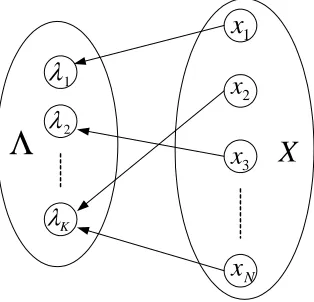
The bipartite graph view (Figure 1) assumes a set of N data objects X (e.g., sequences), represented by x1,x2, ...,and xN, and K probabilistic generative models (e.g., HMMs),λ1,λ2, ...,λK, each
corre-sponding to a cluster of data objects.2The bipartite graph is formed by connections between the data and model spaces. The model space usually contains members of a specific family of probabilistic models. A model λy can be viewed as the generalized “centroid” of cluster y, though it typically
provides a much richer description of the cluster than a centroid in the data space. A connection between an object x and a modelλy indicates that the object x is being associated with cluster y,
with the connection weight (closeness) between them given by the log-likelihood log p(x|λy).
1
λ
2
λ
K
λ
1
x
2
x
3
x
N
x
Λ
X
Figure 1: A bipartite graph view of model-based clustering.
Readers may immediately notice the conceptual similarity between this view and the EM algo-rithm (Dempster et al., 1977), which is a general algoalgo-rithm for solving maximum likelihood esti-mation from incomplete data. Indeed, for partitional clustering, the cluster indices for data objects can be treated as missing data and the EM algorithm can be employed to estimate the model param-eters that maximize the incomplete data likelihood P(X|Λ). The bipartite graph view, however, is not equivalent to the EM algorithm for two reasons. First, it is not an algorithm; rather it provides
2. We interchangeably useλto represent a model as well as the set of parameters of that model. The set of all parameters used for modeling the whole dataset is represented byΛ={λ1, ...,λK}. Later in this paper,Λalso includes cluster
a visualization for model-based clustering. Second, it also encompasses hierarchical model-based clustering which does not involve incomplete data. The idea of representing clusters by models generalizes the standard k-means algorithm, where both data objects and cluster centroids are in the same data space. The models also provide a probabilistic interpretation of clusters, which is a desirable feature in many applications.
A variety of hard and soft assignment strategies can be designed by attaching to each connection an association probability based on the connection weights. For hard clustering these probabilities are either 1’s or 0’s. Intuitively, a suitable objective function is the sum of all connection weights (log-likelihoods) weighted by the association probabilities, which is to be maximized. Indeed, max-imizing this objective function leads to a well-known hard clustering algorithm (Kearns et al., 1997; Li and Biswas, 2002; Banerjee et al., 2003b). We will show in the next section that soft model-based clustering can be obtained by adding entropy constraints to the objective function. Similar to deterministic annealing, a temperature parameter can be used to regulate the softness of data assignments.
1
λ
2
λ
λ
1
x
2
x
3
x
N
x
Λ
X
λ
λ
K
λ
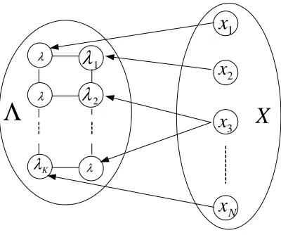
Figure 2: Model-based partitional clustering with an imposed logical neighborhood structure on cluster models.
which can produce balanced clusters, i.e., clusters with comparable number of data objects, and improve clustering quality by using balance constraints in the clustering process.
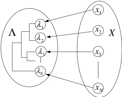
Alternatively, one can initialize K =N and hierarchically merge clusters in the model space,
resulting in a model-based hierarchical clustering algorithm (Figure 3). The difference from the standard single-link or complete-link hierarchical clustering algorithms is that the hierarchy is built in the model space using a suitable measure of divergence between models.
1
λ
2
λ
N
λ
1
x
2
x
3
x
N
x
Λ
X
3
λ
Figure 3:A graph view of model-based hierarchical clustering.
2.2 Model-based Partitional Clustering
In this section, we present a principled, information-theoretic analysis of model-based partitional clustering. The derivation process is similar to that of deterministic annealing (Rose, 1998) and the analysis provides a common view and useful generalization of existing algorithms, including k-means (MacQueen, 1967; Dermatas and Kokkinakis, 1996; Dhillon and Modha, 2001; Li and Biswas, 2002), EM clustering (McLachlan and Basford, 1988; Banfield and Raftery, 1993; Cadez et al., 2000; Meila and Heckerman, 2001), SOM (Kohonen, 1997), and Neural-Gas (Martinetz et al., 1993). The resulting algorithm involves a temperature parameter T , which governs the randomness of posterior data assignments. EM clustering corresponds to the special case T =1 whereas the k-means clustering corresponds to T =0.
Let the joint probability for a data object x and a cluster y be P(x,y). We aim to maximize the expected log-likelihood
L=
∑
x,y
P(x,y)log p(x|λy) =
∑
xP(x)
∑
y
P(y|x)log p(x|λy). (1)
Note that in practice one typically uses a sample average to calculate L, i.e., P(x) = N1,∀x∈X . As N goes to infinity, the sample average approaches the expected log-likelihood asymptotically.
Directly maximizing the objective function in Equation 1 over P(y|x)andλy leads to a known
Lloyd, 1982) and iterates between the following two steps:
P(y|x) =
1, y=arg maxy0log p(x|λy0);
0, otherwise, (2)
and
λy=arg max
λ
∑
x P(y|x)log p(x|λ). (3)The posterior probability P(y|x) in Equation 2 is actually conditioned on current parametersΛ=
{λ1, ...,λK}, but for simplicity we use P(y|x)instead of P(y|x,Λ)where there is no confusion.
Equa-tion 2 represents a hard data assignment strategy— each data object x is assigned, with probability 1, to the cluster y that gives the maximum log p(x|λy). When equi-variant spherical Gaussian models
are used for vector data, the mk-means algorithm reduces to the standard k-means algorithm. It is well known that the k-means algorithm tends to quickly get stuck in a local solution. One way of alleviating this problem is to use soft assignments (Rose, 1998).
To introduce some randomness or softness to the data assignment step, we add entropy con-straints to Equation 1. Let X be the set of all data objects and Y the set of all cluster indices. The new objective is
L1=L+T·H(Y|X)−T·H(Y) =L−T·I(X ;Y), (4) where H(Y) =−∑yP(y)log P(y)is the cluster prior entropy,
H(Y|X) =−
∑
x
P(x)
∑
y
P(y|x)log P(y|x)
the average posterior entropy, and I(X ;Y)the mutual information between X and Y . The parameter
T is a Lagrange multiplier used to trade off between maximizing the average log-likelihood L and
minimizing the mutual information between X and Y . If we fix H(y), minimizing I(X ;Y)is equiv-alent to maximizing the average posterior entropy H(Y|X), or maximizing the randomness of the data assignment.
Note that the added entropy terms do not change the model re-estimation formula in Equation 3 since the model parameters that maximize L also maximize L1. To solve for P(y|x)under constraint
∑yP(y|x) =1, one can first construct the Lagrangian
L
=L1+∑
x
ξx(
∑
y
P(y|x)−1),
where ξ’s are Lagrange multipliers, and then let the partial derivative ∂P∂(Ly|x) =0 .The resulting
P(y|x)is the well-known Gibbs distribution (Geman and Geman, 1984) given by
P(y|x) = P(y)p(x|λy) 1 T
∑y0P(y0)p(x|λy0)
1 T
. (5)
If P(y)is not known a priori, we can estimate it from the data as P(y) =∑xP(x)P(y|x).Now we
Algorithm: model-based clustering via deterministic annealing
Input: A set of N data objects X ={x1, ...,xN}, model structure Λ={λ1, ...,λK}, temperature
decreasing rateα,0<α<1, and final temperature Tf (usually a small positive value close to
0).
Output: Trained modelsΛand a partition of the data objects given by the cluster identity vector
Y ={y1, ...,yN}, yn∈ {1, ...,K}.
Steps:
1. Initialization: initialize the model parametersΛand set T to be high (a large number);
2. Optimization: optimize the objective in Equation 4 by iterating between an E-step (Equa-tion 5) and an M-step (Equa(Equa-tion 3) until convergence;
3. Annealing: lower the temperature parameter T(new)=αT(old), go to step 4 if T<Tf,
other-wise go back to step 2.
4. For each data object xn, set yn=arg maxyP(y|xn).
Figure 4: Deterministic annealing algorithm for model-based clustering.
algorithm for model-based clustering can be constructed as shown in Figure 4. Note that at each temperature, the EM algorithm is used to maximize the objective in Equation 4, with cluster labels Y being the hidden variables and Equation 5 and Equation 3 corresponding to the E-step and M-step, respectively.
It can be shown that plugging Equation 5 into Equation 4 and setting T =1 reduces the objective function to
L∗1=
∑
x
P(x)log
∑
y
P(y)p(x|λy)
!
, (6)
which is exactly the (incomplete data log-likelihood) objective function that the EM clustering max-imizes (Neal and Hinton, 1998). As T goes to 0, Equation 5 reduces to Equation 2 and the algorithm reduces to mk-means, independent of the actual P(y)’s (unless they are 1 and 0’s). For any T >0, iterating between Equation 5 and Equation 3 gives a soft model-based clustering algorithm that maximizes the objective function in Equation 4 for a given T .
A stochastic variant of the mk-means algorithm, stochastic mk-means, was described by Kearns et al. (1997) as posterior assignment (as opposed to k-means assignment and EM assignment). The basic idea is that each data object is stochastically (and entirely, not fractionally) assigned to one of the K clusters according to the posterior probability P(y|x). The stochastic mk-means can also be viewed as a sampled version of the EM clustering, where one uses a sampled E-step based on the posterior probabilities.
We now present a generalized batch version of the SOM and Neural-Gas algorithms in the con-text of model-based clustering and show they also can be interpreted from a deterministic annealing point of view. A distinct feature of SOM is the use of a topological map, in which each cluster has
a fixed coordinate. Let the map location of cluster y beφy and Kα(φy,φy0) =exp
−kφy−φy0k
2
2α2
be
the neighborhood function. Let y(x) =arg maxylog p(x|λy). The batch SOM algorithm amounts to
iterating between Equation 3 and the following step:
P(y|x) = Kα(φy,φy(x))
∑y0Kα(φy0,φy(x)) ,
whereαis a parameter controlling the width of the neighborhood function and decreases gradually during the clustering process. Hereαcan be seen as a temperature parameter as in a deterministic annealing process. SOM can be viewed as using a constrained E-step, where the calculation of posteriors P(y|x)is not only based on the actual log p(x|λy)’s, but also constrained by the topological
map structure. This mechanism gives SOM the advantage that all resulting clusters are related according to the pre-specified topological map.
The batch Neural-Gas algorithm differs from SOM and the algorithm in Figure 4, only in how
P(y|x)is calculated
P(y|x) = e−
r(x,y)/β
∑y0e−r(x,y0)/β
,
whereβis an equivalent temperature parameter and r(x,y)is a function of cluster rank. For example,
r(x,y)takes value 0 if y is the closest cluster centroid to x, value 1 if y is the second closest centroid to x, and value k−1 if y is the k-th closest centroid to x. It has been shown that the online Neural-Gas algorithm can converge faster and find better local solutions than the SOM and deterministic annealing algorithms for certain problems (Martinetz et al., 1993).
2.3 Model-based Hierarchical Clustering
For partitional clustering methods, the number of clusters needs to be specified a priori. This num-ber, however, is often unknown in many clustering problems. Moreover, sometimes one prefers the clustering algorithm to return a series of nested clusterings for interactive analysis (Seo and Shnei-derman, 2002). Hierarchical clustering techniques provide such an advantage. Although one can run k-means or EM clustering multiple times with different numbers of clusters, the returned clusterings are not guaranteed to be structurally related. Bottom-up hierarchical agglomerative clustering has been the most popular hierarchical method (Jain et al., 1999), although top-down methods have also been used, e.g., Steinbach et al. (2000).
hierarchical methods and similarity-based ones. Ward’s algorithm and centroid methods are model-based methods. The former selects two clusters whose merge maximizes the resulting likelihood, whereas the latter chooses the two clusters whose centroids are closest. Both methods use spherical Gaussians as the underlying models. On the other hand, single-link, complete-link, and average-link methods are all discriminative methods, since data-pairwise distances have to be calculated and form the basis for computing inter-cluster distances.
To design model-based hierarchical clustering algorithms, one first needs a methodology for identifying two clusters to merge at each iteration. To do this, we define a “distance”3measure be-tween clusters (i.e., models) and then iteratively merge the closest pair of clusters. A traditional way is to choose the two clusters such that merging them results in the largest log-likelihood log P(X|Λ)
(Fraley, 1999; Meila and Heckerman, 2001). The distance for this method can be defined as
DW(λk,λj) =log P(X|Λbe f ore)−log P(X|Λa f ter), (7)
whereΛbe f oreandΛa f terare the set of all parameters before and after merging two models (λkand
λj), respectively. We call this measure (generalized) Ward’s distance since this is exactly the Ward’s
algorithm (Ward, 1963) when equi-variant Gaussian models are used.
The above method is not efficient, however, since to find the closest pair one needs to train a merged model for every pair of clusters and then evaluate the resulting log-likelihood. In practice, except for some specific models for which the Ward’s distance can be efficiently computed (Fra-ley, 1999; Meila and Heckerman, 2001), the Kullback-Leibler (KL) distance measure which does not involve re-estimating models has been commonly used (Sinkkonen and Kaski, 2001; Ramoni et al., 2002). Exact KL divergence is difficult to calculate for complex4models. An empirical KL divergence (Juang and Rabiner, 1985) between two modelsλk andλj can be defined as
DK(λk,λj) =
1 |Xk|x
∑
∈Xk(log p(x|λk)−log p(x|λj)), (8)
where Xkis the set of data objects being grouped into cluster k. This distance can be made symmetric
by defining (Juang and Rabiner, 1985)
DKs(λk,λj) =
DK(λk,λj) +DK(λj,λk)
2 ,
or using the Jensen-Shannon divergence withπ1=π2=12 (Lin, 1991):
DJS(λk,λj) =
1 2D
K(λ
k,
λk+λj
2 ) + 1 2D
K(λ
j,
λk+λj
2 ).
Compared to classical hierarchical agglomerative clustering (HAC) algorithms, KL divergence is analogous to the centroid method. It can be shown that when Gaussian models with equal co-variance matrices are used, the KL divergence reduces to the Mahalanobis distance between two cluster means. Motivated by this observation as well as the single-link and complete-link HAC
3. This and several other quantities defined in this section that are used as merging criteria are termed “distance” only in a colloquial sense, since they may not satisfy the symmetry or triangle inequality properties needed of a metric. “Divergence” is the technically correct term in such situations.
algorithms, we propose several modified KL distances. Corresponding to single-link, we define a
minKL distance as
Dm(λk,λj) =min x∈Xk
(log p(x|λk)−log p(x|λj)), (9)
and corresponding to complete-link, we define a maxKL distance as
DM(λk,λj) =max x∈Xk
(log p(x|λk)−log p(x|λj)). (10)
Finally, to characterize high “boundary density” between two clusters for building complex-shaped clusters, we propose a boundaryKL distance measure
DB(λk,λj) =
1 |Bk|x
∑
∈Bk(log p(x|λk)−log p(x|λj)), (11)
where Bk is theηfraction of Xk that have smallest log p(x|λk)−log p(x|λj) values. A value of 0
for log p(x|λk)−log p(x|λj)defines the “boundary” between cluster k and j. This distance measure
reduces to the minKL distance if Bkcontains only one data object, and to the KL distance if Bk=Xk.
The minKL and maxKL measures are more sensitive to outliers than the KL distance since they are defined on only one specific data object. A favorable property of the minKL measure, however, is that hierarchical algorithms using this distance (analogous to single-link HAC methods) can produce arbitrary-shaped clusters. To guard against outliers but reap the benefits of single-link methods, we setηto be around 10%. The experimental results in Section 6 demonstrate the effectiveness of this new distance measure.
Figure 5 describes a generic view of model-based HAC algorithm. Instances of this generic algorithm include existing model-based HAC algorithms that were first explored by Banfield and Raftery (1993) and Fraley (1999) with Gaussian models, later by Vaithyanathan and Dom (2000) with multinomial models for clustering documents, and more recently by Ramoni et al. (2002) with Markov chain models for grouping robot sensor time series. The first three works used the Ward’s distance in Equation 7 and the fourth one employed the KL distance in Equation 8.
2.4 Practical Considerations
In general, the maximum likelihood estimation of model parameters in Equation 2 can itself be an iterative optimization process (e.g., estimation of HMMs), that needs appropriate initialization and may get into local minima. For the clustering algorithms to converge, sequential initialization has to be used. That is, the model parameters resulting from the previous clustering iteration should be used to initialize the current clustering iteration, to guarantee that the objective (Equation 1 or 4) does not decrease.
The second observation is that ML model estimation sometimes leads to a singularity prob-lem, i.e., unbounded log-likelihood. This can happen for a continuous probability distribution for which p(x|λ)is a probability density that can become unbounded even thoughR
xp(x|λ)dx=1. For
Algorithm: model-based HAC
Input: A set of N data objects X={x1, ...,xN}, and model structureλ.
Output: An N-level cluster (model) hierarchy and hierarchical partition of the data objects, with n models/clusters at the n-th level.
Steps:
1. Initialization: start with the N-th level, initialize each data object as a cluster itself and train a model for each cluster, i.e.,λn=max
λ log p(xn|λ);
2a. Distance calculation: compute pairwise inter-cluster distances using an appropriate measure, e.g., one of the measures defined in Equations 7–11;
2b. Cluster merging: merge the two closest clusters (assume they are k and j) and re-estimate a model from the merged data objects Xk=Xk∪Xj, i.e.,λk=max
λ log P(Xk|λ);
3. Stop if all data objects have been merged into one cluster, otherwise go back to Step 2a.
Figure 5: Model-based hierarchical agglomerative clustering algorithm.
A third comment is on the performance of mk-means, stochastic mk-means, and EM cluster-ing. In practice, it is common to see the condition p(x|λy(x)) p(x|λk),∀k6=y(x)(especially for
complex models such as HMMs), which means that P(k|x)in Equation 5 will be dominated by the likelihood values and be very close to 1 for k=y(x),and 0 otherwise, provided that T is small (≤1). This suggests that the differences between hard mk-means, stochastic mk-means, and EM clustering algorithms are often small, i.e., their clustering results will be similar in many practical applications.
Finally, let us look at the computational complexity for model-based clustering algorithms. First consider partitional clustering involving models for which the estimation of model parameters has a closed-form solution and does not need an iterative process, e.g., Gaussian, Multinomial, etc. For each iteration, the time complexity is linear in the number of data objects N and the number of clusters K for both the data assignment step and the model estimation step. The total complexity is O(KNM), where M is the number of iterations. For those models for which the estimation of parameters needs an iterative process (e.g., hidden Markov models with Gaussian observation den-sity), the model estimation complexity is O(KNM1)for each clustering iteration, where M1is the number of iterations used in the model estimation process. In this case, the total complexity of the clustering process is O(KNMM1). Theoretically the number of iterations M and M1could be very large and may increase a bit with N, but in practice the maximum number of iterations is typically set to be a constant based on empirical observations. In our experiments, the EM algorithm usually converges very fast (within 20 to 30 iterations when clustering documents).
The above analysis applies to mk-means, stochastic mk-means, and EM clustering. For the model-based deterministic annealing algorithm, there is an additional outer loop controlled by the decreasing temperature parameter. Therefore, a slower annealing schedule is computationally more expensive.
calculated isN(N2−1)for the bottom (N-th) level and i−1 for the i-th level (i<N, other than the N-th
level, one only needs to compute the distances between the merged cluster and other clusters). The total number of distances calculated for the whole hierarchy is
N(N−1)
2 + (N−2) + (N−3) +···+1'O(N 2).
Using the same logic, we can compute the total number of distance comparisons needed as
N(N−1)
2 +
(N−1)(N−2)
2 +···+
2·1
2 'O(N 3), and the total complexity for model estimation as
N·1M1+1·2M1+1·3M1+···+1·NM1'O(N2M1),
where M1 is the number of iterations used for model estimation. The complexity can be reduced to O(N2log N)for inter-cluster distance comparisons by using a clever data structure (e.g., heap) to store the comparison results (Jain et al., 1999). Clearly, a complexity of O(N3) or O(N2log N)is still too high for large datasets, which explains why model-based hierarchical clustering algorithms are not as popular as partitional ones. In areas where researchers do use hierarchical algorithms, model-specific tricks have often been used to further reduce the computational complexity (Fraley, 1999; Meila and Heckerman, 2001).
3. Clustering Evaluation
Comparative studies on clustering algorithms are difficult in general due to lack of universally agreed upon quantitative performance evaluation measures (Jain et al., 1999). Subjective (human) evaluation is often difficult and expensive, yet is still indispensable in many real applications. Ob-jective clustering evaluation criteria include intrinsic measures and extrinsic measures (Jain et al., 1999). Intrinsic measures formulate quality as a function of the given data and similarities/models and are often the same as the objective function that a clustering algorithm explicitly optimizes. For example, the data likelihood objective was used by Meila and Heckerman (2001) to cluster text data using multinomial models. For low-dimensional vector data, the average (or summed) distance from cluster centers, e.g., the sum-squared error criteria used for the standard k-means algorithm, is a common criterion.
Extrinsic measures are commonly used when the category (or class) labels of data are known (but of course not used in the clustering process). In this paper, a class is a predefined (“true”) data category but a cluster is a category generated by a clustering algorithm. Examples of external measures include the confusion matrix, classification accuracy, F1 measure, average purity, average entropy, and mutual information (Ghosh, 2003). There are also several other ways to compare two partitions of the same data set, such as the Rand index (Rand, 1971) and Fowlkes-Mallows measure (Fowlkes and Mallows, 1983) from the statistics community.
is 0. If a cluster contains an equal number of objects from each category, the purity is 1/K and the
normalized entropy is 1.
It has been argued that the mutual information I(Y ; ˆY) between a r.v. Y , governing the cluster labels, and a r.v. ˆY , governing the class labels, is a superior measure to purity or entropy (Dom,
2001; Strehl and Ghosh, 2002). Moreover, by normalizing this measure to lie in the range [0,1], it becomes relatively impartial to K. There are several choices for normalization based on the entropies
H(Y) and H(Yˆ). We shall follow the definition of normalized mutual information (NMI) using geometrical mean, NMI= √I(Y ; ˆY)
H(Y)·H(Yˆ), as given by Strehl and Ghosh (2002). The corresponding sample estimate is:
NMI= ∑h,l
nh,llog
n
·nh,l
nhnl
q
∑hnhlognnh
∑lnllognnl
,
where nhis the number of data objects in class h, nl the number of objects in cluster l and nh,l the
number of objects in class h as well as in cluster l. The NMI value is 1 when clustering results perfectly match the external category labels and close to 0 for a random partitioning.
In the simplest scenario where the number of clusters equals the number of categories and their one-to-one correspondence can be established, any of these external measures can be fruitfully applied. For example, when the number of clusters is small (<4), the accuracy measure is intuitive and easy to understand. However, when the number of clusters differs from the number of original classes, the confusion matrix is hard to read and the accuracy difficult (or sometimes impossible) to calculate. In such situations, the NMI measure is better than purity and entropy measures, both of which are biased towards high k solutions (Strehl et al., 2000; Strehl and Ghosh, 2002).
In this paper, several different measures are used, and we explain in each case study what mea-sures we use and why.
4. A Case Study on Document Clustering
We recently performed an extensive comparative study of model-based approaches to document clustering (Zhong and Ghosh, 2003a). This section reports on a small subset of this study with an intent to highlight how the unified framework proves very helpful in such an endeavor. Therefore, details of the data sets, experimental setting and comparative results are relegated to Zhong and Ghosh (2003a) while we focus here on the experimental process. In particular, we compare two different probabilistic model types, namely mixtures of multinomials and of von-Mises Fisher dis-tributions. For each model type, we instantiate the four generic model-based clustering algorithms (mk-means, stochastic mk-means, EM, and deterministic annealing) described in Section 2.2. The key observation is that the same pseudocode of mk-means (Figure 6) can be used for different models— only the model re-estimation segment (Step. 2a) needs to be changed. Thus, code devel-opment becomes easier and experimental settings can be automatically kept the same for different models to ensure a fair comparison.
The traditional vector space representation is used for text documents, i.e., each document is represented as a high dimensional vector of “word”5 counts in the document. The dimensionality equals the number of words in the vocabulary used.
Algorithm: mk-means
Input: Data objects X={x1, ...,xN}, and model structureΛ={λ1, ...,λK}.
Output: Trained model parametersΛand a partition of the data samples given by the cluster iden-tity vector Y={y1, ...yN},yi∈ {1, ...,K}.
Steps:
1. Initialization: initialize the model parametersΛand cluster identity vector Y ;
2a. Model re-estimation: for each cluster j, let Xj={xi|yi=j}, the parameters of each modelλj
is re-estimated asλj=max
λ ∑x∈Xjlog p(x|λ);
2b. Sample re-assignment: for each data sample i, set yi=arg max
j log p(xi|λj);
3. Stop if Y does not change, otherwise go back to Step 2a.
Figure 6:Common mk-means template for document clustering case study.
4.1 Models
Multinomial models have been quite popular for text clustering (Meila and Heckerman, 2001), and we use the standard formulation for estimating the model parameters following McCallum and Nigam (1998), who use Laplace smoothing to avoid zero probabilities. The second model uses the von Mises-Fisher distribution, which is the analogue of the Gaussian distribution for directional data in the sense that it is the unique distribution of L2-normalized data that maximizes the entropy given the first and second moments of the distribution (Mardia, 1975). There is a long-time folklore in the information retrieval community that the direction of a text vector is more important than its magnitude, leading to the practices of using cosine similarity, and of normalizing such vectors to unit length using L2norm. Thus a model for directional data seems worthwhile to consider. The pdf of a vMF distribution is
p(x|λ) = 1
Z(κ)exp κ·x
Tµ
,
where x is a L2-normalized data vector, µ the L2-normalized mean vector, and the Bessel function
Z(κ)a normalization term. Theκmeasures the directional variance (or dispersion) and the higher it is, the more peaked the distribution is. The maximum likelihood estimation of µ is simple and given by µ= ∑x
k∑xk. The estimation ofκ, however, is rather difficult due to the Bessel function involved
(Banerjee and Ghosh, 2002a; Banerjee et al., 2003a). In a k-means clustering setting, ifκis assumed to be the same for all clusters, then the clustering results do not depend onκ, which can be ignored. In this case, we can evaluate the average cosine similarity (N1∑xxTµ, which is actually a displaced
log-likelihood) as the objective (to be minimized). For EM clustering, the maximum likelihood so-lution has been derived by Banerjee et al. (2003a) including the computationally expensive updates forκ. In this work, for convenience, we use a simpler soft assignment scheme, which is discussed in Section 4.3. To use vMF models, the word-count document vectors are log(IDF)-weighted and then L2-normalized. The IDF here stands for inverse document frequency. The log(IDF) weighting is a common practice in the information retrieval community used to de-emphasize the words that occur in too many documents. The weight for word l is logNN
l, where N is the number of documents
vMF distribution is a directional distribution defined on a unit hypersphere and does not capture any magnitude information.
4.2 Datasets
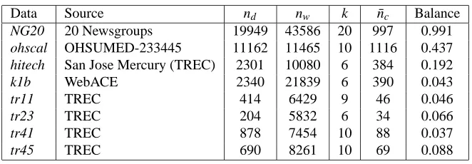
We used the 20-newsgroups dataset6and a number of datasets from the CLUTO toolkit7(Karypis, 2002). These datasets provide a good representation of different characteristics: the number of documents ranges from 204 to 19949, the number of terms from 5832 to 43586, the number of classes from 6 to 20, and the balance from 0.037 to 0.991. Here the balance of a dataset is defined as the ratio of the number of documents in the smallest class to the number of documents in the largest class. So a value close to 1(0) indicates a very (un)balanced dataset. A summary of all the datasets used in this section is shown in Table 1. Additional details on data characteristics and preprocessing are found work by Zhao and Karypis (2001) and Zhong and Ghosh (2003a).
Data Source nd nw k n¯c Balance
NG20 20 Newsgroups 19949 43586 20 997 0.991
ohscal OHSUMED-233445 11162 11465 10 1116 0.437
hitech San Jose Mercury (TREC) 2301 10080 6 384 0.192
k1b WebACE 2340 21839 6 390 0.043
tr11 TREC 414 6429 9 46 0.046
tr23 TREC 204 5832 6 34 0.066
tr41 TREC 878 7454 10 88 0.037
tr45 TREC 690 8261 10 69 0.088
Table 1: Summary of text datasets. (For each dataset, nd is the total number of documents, nwthe
total number of words, k the number of classes, and ¯ncthe average number of documents
per class.)
4.3 Experiments
For simplicity, we introduce some abbreviations: when instantiated with the multinomial model, the four algorithms— mk-means, stochastic mk-means, EM, and deterministic annealing— will be referred to as k-multinomials (kmnls), stochastic k-multinomials (skmnls), mixture-of-multinomials (mixmnls), and multinomial-based deterministic annealing (damnls), respectively. For vMF-based algorithms, the corresponding abbreviated names are kvmfs, skvmfs, softvmfs, and davmfs. We use softvmfs instead of mixvmfs for the soft vMF-based algorithm for the following reason. As mentioned previously, the estimation of parameterκin a vMF model is difficult but is needed for the mixture-of-vMFs algorithm. As a simple heuristic, we useκm=20m, where m is the iteration
number. Soκis set to be a constant for all clusters at each iteration, and gradually increases over iterations.
The davmfs algorithm uses an exponential schedule for the (equivalent) inverse temperature parameterκ, i.e.,κm+1=1.1κm, starting from 1 and up to 500. For the damnls algorithm, an inverse
temperature parameterγ=1/T is created to parameterize the E-step of mixmnls. The annealing
schedule forγis set toγm+1=1.3γm, andγstarts from 0.5 and can go up to 200.
For all the model-based algorithms, we use a relative convergence criterion— when the likeli-hood objective changes less than 0.01% for the multinomial models or the average cosine similarity less than 0.1% for the vMF models, the iterative process is treated as converged. For all situations except the vMF models on the NG20 dataset, the clustering process converges in 20 or fewer iter-ations on average. The largest average number of iteriter-ations needed is 38, for the skvmfs algorithm running on NG20 with 30 clusters. Each experiment is run ten times, each time starting from a random balanced partition of documents. The averages and standard deviations of the normalized mutual information results are reported. We use NMI measure since the class labels of each doc-ument are available and the number of clusters is relatively large. Recall that NMI measures how well the clustering results match existing category labels. We also include the results for one state-of-the-art graph partitioning approach to document clustering— CLUTO (Karypis, 2002). We use the vcluster algorithm in the CLUTO toolkit with default setting. The algorithm is run ten times, each time with randomly ordered documents. Note that results of regular k-means (using Euclidean distance) are not included since this is well known to perform miserably for high-dimensional text data (Strehl et al., 2000).
4.4 Discussion
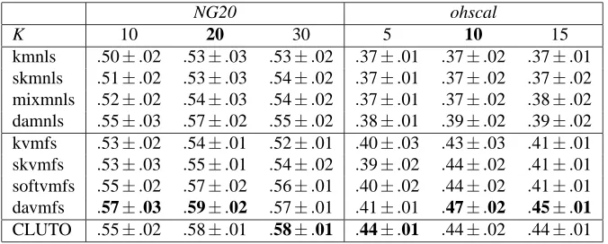
Table 2 shows the NMI results on the NG20 and ohscal datasets, across different number of clusters for each dataset. All numbers in the table are shown in the format average±1 standard deviation.
Boldface entries highlight the best performance in each column. The number of clusters K does not seem to affect much the relative comparison between different algorithms, at least for the range of K we have experimented with in this study. This is also the case for other datasets (Zhong and Ghosh, 2003a). Therefore, to save space, we show the NMI results on all other datasets for one specific K only in Table 3.
NG20 ohscal
K 10 20 30 5 10 15
kmnls .50±.02 .53±.03 .53±.02 .37±.01 .37±.02 .37±.01 skmnls .51±.02 .53±.03 .54±.02 .37±.01 .37±.02 .37±.02 mixmnls .52±.02 .54±.03 .54±.02 .37±.01 .37±.02 .38±.02 damnls .55±.03 .57±.02 .55±.02 .38±.01 .39±.02 .39±.02 kvmfs .53±.02 .54±.01 .52±.01 .40±.03 .43±.03 .41±.01 skvmfs .53±.03 .55±.01 .54±.02 .39±.02 .44±.02 .41±.01 softvmfs .55±.02 .57±.02 .56±.01 .40±.02 .44±.02 .41±.01 davmfs .57±.03 .59±.02 .57±.01 .41±.01 .47±.02 .45±.01 CLUTO .55±.02 .58±.01 .58±.01 .44±.01 .44±.02 .44±.01
Table 2: NMI results on NG20 and ohscal dataset
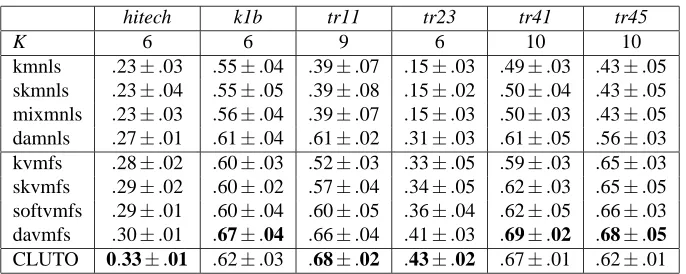
hitech k1b tr11 tr23 tr41 tr45
K 6 6 9 6 10 10
kmnls .23±.03 .55±.04 .39±.07 .15±.03 .49±.03 .43±.05 skmnls .23±.04 .55±.05 .39±.08 .15±.02 .50±.04 .43±.05 mixmnls .23±.03 .56±.04 .39±.07 .15±.03 .50±.03 .43±.05 damnls .27±.01 .61±.04 .61±.02 .31±.03 .61±.05 .56±.03 kvmfs .28±.02 .60±.03 .52±.03 .33±.05 .59±.03 .65±.03 skvmfs .29±.02 .60±.02 .57±.04 .34±.05 .62±.03 .65±.05 softvmfs .29±.01 .60±.04 .60±.05 .36±.04 .62±.05 .66±.03 davmfs .30±.01 .67±.04 .66±.04 .41±.03 .69±.02 .68±.05 CLUTO 0.33±.01 .62±.03 .68±.02 .43±.02 .67±.01 .62±.01
Table 3: NMI Results on hitech, k1b, tr11, tr23, tr41, and tr45 datasets
Zhong and Ghosh (2003a) indicates that algorithms using soft assignment take (slightly) longer time than those using hard assignments. While the kvmfs algorithm is the fastest overall, deterministic annealing is much slower for vMF distributions.
5. Balanced Model-based Clustering
The problem of clustering large scale data under constraints such as balancing has recently received attention in the data mining literature (Bradley et al., 2000; Tung et al., 2001; Banerjee and Ghosh, 2002b; Strehl and Ghosh, 2003; Zhong and Ghosh, 2003b). Balanced solutions yield comparable numbers of objects in each cluster, and are desirable in a variety of applications (Zhong and Ghosh, 2003b). However, since balancing is a global property, it is difficult to obtain near-linear time techniques to achieve this goal while retaining high cluster quality. In this section we show how balancing constraints can be readily incorporated into the unified framework. Essentially, one needs to perform a balanced partitioning of the bipartite graph (Figure 1) at each iteration of the EM algorithm, i.e., use a balanced E-step. The suggested approach can be easily generalized to handle partially balanced assignments and specific percentage assignment problems.
5.1 Balanced Model-based K-means
Since we focus on balanced hard clustering, the posteriors are either 1’s or 0’s. For simplicity, let
znk be a binary assignment variable with a value of 1 indicating that data object xnis assigned to
cluster k. The completely balanced mk-means clustering problem can then be written as:
max
{λ,z} n∑,k
znklog p(xn|λk)
s.t. ∑kznk=1,∀n; ∑nznk=N/K,∀k;
znk∈ {0,1},∀n,k.
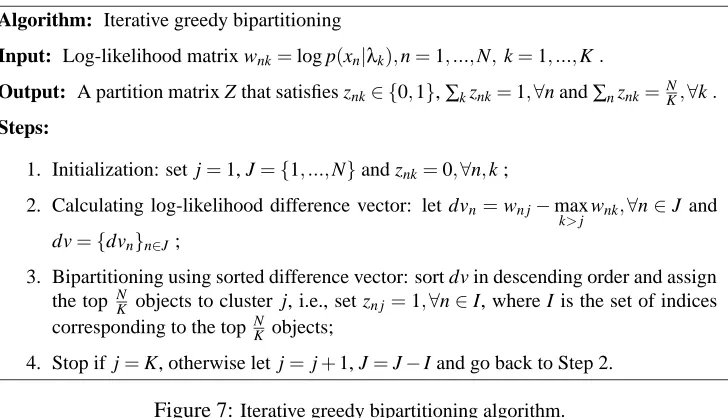
Algorithm: Iterative greedy bipartitioning
Input: Log-likelihood matrix wnk=log p(xn|λk),n=1, ...,N, k=1, ...,K.
Output: A partition matrix Z that satisfies znk∈ {0,1},∑kznk=1,∀n and∑nznk=NK,∀k.
Steps:
1. Initialization: set j=1, J={1, ...,N}and znk=0,∀n,k ;
2. Calculating log-likelihood difference vector: let dvn=wn j−max
k>jwnk,∀n∈J and
dv={dvn}n∈J;
3. Bipartitioning using sorted difference vector: sort dv in descending order and assign the top NK objects to cluster j, i.e., set zn j=1,∀n∈I, where I is the set of indices
corresponding to the topNK objects;
4. Stop if j=K, otherwise let j=j+1, J=J−I and go back to Step 2.
Figure 7:Iterative greedy bipartitioning algorithm.
and M-step in the EM algorithm, respectively. The balanced data assignment subproblem is
max
{z} n∑,k
znklog p(xn|λk)
s.t. ∑kznk=1,∀n; ∑nznk=N/K,∀k;
znk∈ {0,1},∀n,k.
(12)
This is an integer programming problem, which is NP-hard in general. Fortunately, this integer programming problem is special in that it has the same optimum as its corresponding real relaxation (Bradley et al., 2000), which is a linear programming problem. The best known exact algorithm to solve this linear programming problem is an improved interior point method that has a complexity of O(N3K3/log(NK)), according to Anstreicher (1999).
To make this clustering algorithm scalable to large database, we seek approximate solutions (to the optimization problem in Equation 12) that can be obtained in time better than O(N2). We propose an iterative greedy bipartitioning algorithm (Figure 7) that assigns N/K data objects to one
of the K clusters at each iteration in a locally optimal fashion.
The motivation behind this heuristic is that it solves the balanced assignment problem (Equa-tion 12) exactly for K =2. In other words, if there are just two clusters, one simply sorts the difference vector dvn=log p(xn|λ1)−log p(xn|λ2),n=1, ...,N in descending order and assigns the first N/2 objects to cluster 1 and the second half to cluster 2. It is easy to show that this gives a {N
2,
N
2} bipartition that maximizes the objective in Equation 12. For K>2, a greedy bipartition is conducted at each iteration that separates the data objects for one cluster from all the others in such a way that the objective in Equation 12 is locally maximized. It is trivial to show that the j-th iteration of the algorithm in Figure 7 gives a locally optimal{NK,(K−Kj)N}bipartition that assigns NK objects to the j-th cluster.
Let us now look at the time complexity of this algorithm. Let Nj = (K+1K−j)N be the length
of the difference vector computed at the j-th iteration. Calculating the difference vectors takes
time complexity is O(K2N+KN log N) for the greedy bipartitioning algorithm and O(K2MN+ KMN log N) for the resulting balanced clustering algorithm, where M is the number of clustering iterations. The greedy nature of the algorithm stems from the imposition of an arbitrary ordering of the clusters using j. So one should investigate the effect of different orderings. In the experiments, the ordering is done at random in each experiment, multiple experiments are run and the variation in results is inspected. The results exhibit no abnormally large variations and suggest that the effect of ordering is small.
A post-processing refinement can be used to improve cluster quality when approximate rather than exact balanced solutions are acceptable. This is achieved by letting the results from completely balanced mk-means serve as an initialization for the regular mk-means. Since the regular mk-means has relatively low complexity of O(KMN), this extra overhead is low. The experiments reported in this section reflect a “full” refinement in the sense that the regular mk-means in the refinement step is run until convergence. Alternatively, partial refinement such as one round of ML re-assignment can be used and is expected to give an intermediate result between the completely balanced one and the “fully” refined one. In the experimental results, intermediate results are not shown but they will be bounded from both sides by the completely balanced and the “fully” refined results.
The refinement step can be viewed from a second perspective— results from completely bal-anced clustering serve as an initialization to regular mk-means clustering. From this point of view, the completely balanced data assignment generates better initial clusters than random initialization according to our experimental results.
5.2 Results on Real Text Data
We used the NG20 dataset described in Section 4.2, and two types of models, vMFs and multinomi-als. For each model type, we compare the balanced mk-means with regular mk-means clustering in terms of balance, objective value and mutual information with original labels, over different num-ber of clusters. The balance of a clustering is defined as the normalized entropy of cluster size distribution of the clustering, i.e.,
Nentro=−
1 log K
K
∑
k=1
Nk
N log
Nk
N
,
where Nkis the number of data objects in cluster k. A value of 1 means perfectly balanced
cluster-ing and 0 extremely unbalanced clustercluster-ing. The average log-likelihood of a clustercluster-ing is given by 1
N∑x∑dl=1x(l)log P
(y)
l for multinomial models and by
1
N∑xxTµyfor von Mises-Fisher models, where
y=arg maxy0p(x|λy0)and d is the dimensionality of document vectors. Other experimental settings
are the same as in Section 4.3.
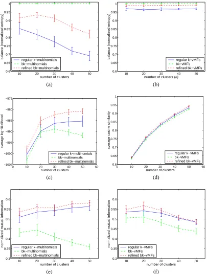
Figure 8 show the results on the NG20 dataset, with results for multinomial models on the left column and those for vMF models on the right. The first row shows balance results (normalized entropy), the second row average log-likelihood (ALL) values and the last row normalized mutual information (NMI) values. All results are shown as average±1 standard deviation over 20 runs.
10 20 30 40 50 0.6 0.65 0.7 0.75 0.8 0.85 0.9 0.95 1
number of clusters
balance (normalized entropy) regular k−multinomials
bk−multinomials refined bk−multinomials
10 20 30 40 50 0.6 0.65 0.7 0.75 0.8 0.85 0.9 0.95 1
number of clusters (k)
balance (normalized entropy) regular k−vMFs
bk−vMFs refined bk−vMFs
(a) (b)
0 10 20 30 40 50 60
−1005 −1000 −995 −990 −985 −980 −975
number of clusters
average log−likelihood
regular k−multinomials bk−multinomials refined bk−multinomials
0 10 20 30 40 50 60 0.6 0.65 0.7 0.75 0.8 0.85 0.9 0.95 1
number of clusters
average cosine similarity
regular k−vMFs bk−vMFs refined bk−vMFs
(c) (d)
10 20 30 40 50 0.3 0.35 0.4 0.45 0.5 0.55 0.6
number of clusters
normalized mutual information regular k−multinomials
bk−multinomials refined bk−multinomials
10 20 30 40 50 0.3 0.35 0.4 0.45 0.5 0.55 0.6
number of clusters
normalized mutual information regular k−vMFs
bk−vMFs refined bk−vMFs
(e) (f)
clusterings than the regular mk-means. Comparing multinomial models with vMF ones, we see that the vMF-based algorithms produce much more balanced clusterings for all datasets.
Note that the balanced variation of model-based clustering is generic since it is applied on the unified framework. One can simply plug in different models for different applications. For conciseness, we have only shown results on one dataset here. More experimental results can be found in an earlier paper (Zhong and Ghosh, 2003b).
6. Hybrid Model-based Clustering
This section presents a hybrid methodology that combines the advantages of partitional and hierar-chical methods. The idea is a “reverse” of the “Scatter/Gather” approach (Cutting et al., 1992) and has been used by Vaithyanathan and Dom (2000) and Karypis et al. (1999). We shall first analyze the advantages of this hybrid approach for model-based clustering, and then present a new variation called hierarchical meta-clustering in Section 6.1. Two case studies are presented in Section 6.2 and 6.3 to show the benefits of hybrid model-based clustering algorithms. The key observation, how-ever, is that the hybrid methodology is built on top of the generic partitional model of Section 2.2 and thus inherits its generality.
Figure 9 shows a generic model-based hybrid algorithm. We first cluster the data into K0(greater than the “natural” number of clusters K, which may be unknown) groups, that is, cluster the data into fine granularity, using a partitional method discussed in Section 2.2. For model-based clustering, this means that we now have K0models. The first step can be viewed as compressing/coarsening of the data. In the second step, we run the HAC algorithm starting from the K0clusters to iteratively merge the clusters that are closest to each other until all data objects are in one cluster or the process is stopped by a user. This hybrid approach returns a series of nested clusterings that can be either interactively analyzed by the user or evaluated with an optimization criterion. Note the methodology is not necessarily limited to model-based clustering (Karypis et al., 1999) although we only intend to show the benefits of model-based approaches in this paper.
This hybrid algorithm is a practical substitute for hierarchical agglomerative clustering algo-rithm since it keeps some hierarchical structure and the visualization benefit but reduces compu-tational complexity from O(N3)to O(K03+K0NM1).8 We can reasonably set K0 to be a constant times K to obtain the same complexity as model-based partitional clustering (assuming K0N).
It can also be used to improve partitional clustering algorithms by starting at K0 clusters and it-eratively merge back to K clusters. This method has proven to be effective for graph partitioning techniques to generate high quality partitions (Karypis et al., 1999). An intuitive explanation is that the second merging step fine-tunes and improves the initial flat clusters. Experimental results in Section 6.3 show the effectiveness of the hybrid clustering approach on time series clustering with hidden Markov models.
In the next section, we introduce a particular variation of this hybrid algorithm— a hierarchical meta-clustering algorithm.
8. The number of distance comparisons is O(K03)and the complexity for estimating models is O(K0NM1)following the
Algorithm: model-based hybrid partitional-hierarchical clustering
Input: Data objects X={x1, ...,xn}, model structureλand hierarchy depth K0.
Output: A K0level cluster (model) hierarchy and hierarchical partition of the data objects, with i
clusters at the i-th level.
Steps:
1. Flat partitional clustering: partition data objects into K0clusters using one of the model-based
partitional clustering algorithms discussed in Section 2.2;
2a. Distance calculation: compute pairwise inter-cluster distances using one of the measures defined in Equations 8–11, and identify the closest cluster pair;
2b. Cluster merging: merge the two closest clusters (assume they are j and j0) and re-estimate a model for the merged data objects Xj=Xj∪Xj0, i.e., letλj=arg max
λ log P(Xj|λ);
3. Stop if all data objects have been merged into one cluster or user-specified number of clusters is reached, otherwise go back to Step 2a.
Figure 9:Model-based hybrid partitional-hierarchical clustering algorithm.
6.1 Hierarchical Meta-clustering
Let us first introduce a composite modelλj j0 ={λj,λj0}for the cluster merged from cluster j and
j0 and define the likelihood of a data object x given this model as
p(x|λj j0) =max{p(x|λj),p(x|λj0)}. (13)
Let us callλj andλj0 children of the composite modelλj j0. For the set of data objects in the merged
cluster Xj j0 =Xj∪Xj0, we then have
log p(Xj j0|λj j0) =log p(Xj|λj) +log p(Xj0|λj0). (14)
Furthermore, we define the distance between two composite modelsλa={λa1,λa2, ...}andλb=
{λb1,λb2, ...}to be
D(λa,λb) =min
λ∈λa
λ0∈λb
D(λ,λ0). (15)
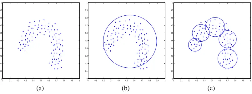
Two immediate benefits result from the above design. First, no model (parameter) re-estimation is needed after merging two clusters, since a composite model is simply represented by the parame-ters of its children. From Equation 14, it can be seen that now the cluster merging does not change the likelihood P(X|Λ), which also means that the Ward’s distance (Equation 7) cannot be used in this case. Second, a composite model can be used to characterize complex clusters that a single model represents poorly. For example, a (rotated) u-shape cluster (Figure 10) cannot be accurately modeled by a single Gaussian but can be approximated by a mixture of Gaussians. Using a sin-gle Gaussian model loses the u-shape structure of the cluster whereas concatenating five spherical Gaussian clusters gives a good representation, as shown in Figure 10(b) & (c).
0 0.1 0.2 0.3 0.4 0.5 0.6 0.7 0.8 0.9 1 0
0.1 0.2 0.3 0.4 0.5 0.6 0.7 0.8 0.9 1
0 0.1 0.2 0.3 0.4 0.5 0.6 0.7 0.8 0.9 1 0
0.1 0.2 0.3 0.4 0.5 0.6 0.7 0.8 0.9 1
0 0.1 0.2 0.3 0.4 0.5 0.6 0.7 0.8 0.9 1 0
0.1 0.2 0.3 0.4 0.5 0.6 0.7 0.8 0.9 1
(a) (b) (c)
Figure 10: (a) A u-shape cluster. (b) Using a single spherical Gaussian model for the cluster. (c) Using a union of five spherical Gaussian models for the cluster. (Each circle shows the isocontour of a Gaussian model at two times the standard deviation.)
cluster as a meta-object and applying the traditional single-link hierarchical clustering algorithm to group the meta-objects. Obviously, nothing prevents us from using a different hierarchical method (e.g., complete-link, average-link, etc.) to cluster the meta-objects, by suitably modifying the mea-sure definition in Equation 15. Each hierarchical method can be desirable in different applications.
The hierarchical meta-clustering algorithms can be seen as a combination of model-based flat clustering and discriminative hierarchical methods. Compared to using a single complex model, we favor this strategy of merging simple models to form complex clusters when a single complex model is difficult to define and to train. For example, what is the distribution for the u-shape cluster in Figure 10(a)? Furthermore, it is almost impossible to avoid poor local solutions even if we can define such a complex distribution.
It is sometimes helpful to produce approximately balanced clusters in the first (partitional) step. This may not be immediately clear, so let us again look at the u-shape cluster in Figure 10(a) as an example. Suppose we divide the data into five clusters in the flat clustering step. Using the k-means algorithm, we may get a very unbalanced clustering that contains one big cluster as in Figure 10(b) and four other near empty clusters (not shown), or a balanced solution as in Figure 10(c). While merging the five clusters back to one in either solution leads to the same set of data objects, we prefer the latter solution since it provides a useful hierarchy, disclosing the u-shape structure of the cluster.
6.2 Results on Synthetic 2-D Spatial Data