A Fast Hybrid Algorithm for Large-Scale
ℓ
1-Regularized
Logistic Regression
Jianing Shi [email protected]
Department of Biomedical Engineering Columbia University
New York, NY 10025, USA
Wotao Yin [email protected]
Department of Computational and Applied Mathematics Rice University
Houston, TX 77005, USA
Stanley Osher [email protected]
Department of Mathematics
University of California Los Angeles Los Angeles, CA 90095, USA
Paul Sajda [email protected]
Department of Biomedical Engineering Columbia University
New York, NY 10025, USA
Editor: Saharon Rosset
Abstract
ℓ1-regularized logistic regression, also known as sparse logistic regression, is widely used in ma-chine learning, computer vision, data mining, bioinformatics and neural signal processing. The use ofℓ1regularization attributes attractive properties to the classifier, such as feature selection, robust-ness to noise, and as a result, classifier generality in the context of supervised learning. When a sparse logistic regression problem has large-scale data in high dimensions, it is computationally ex-pensive to minimize the non-differentiableℓ1-norm in the objective function. Motivated by recent work (Koh et al., 2007; Hale et al., 2008), we propose a novel hybrid algorithm based on combin-ing two types of optimization iterations: one becombin-ing very fast and memory friendly while the other being slower but more accurate. Called hybrid iterative shrinkage (HIS), the resulting algorithm is comprised of a fixed point continuation phase and an interior point phase. The first phase is based completely on memory efficient operations such as matrix-vector multiplications, while the second phase is based on a truncated Newton’s method. Furthermore, we show that various optimization techniques, including line search and continuation, can significantly accelerate convergence. The algorithm has global convergence at a geometric rate (a Q-linear rate in optimization terminology). We present a numerical comparison with several existing algorithms, including an analysis using benchmark data from the UCI machine learning repository, and show our algorithm is the most computationally efficient without loss of accuracy.
1. Introduction
Logistic regression is an important linear classifier in machine learning and has been widely used in computer vision (Bishop, 2007), bioinformatics (Tsuruoka et al., 2007), gene classification (Liao and Chin, 2007), and neural signal processing (Parra et al., 2005; Gerson et al., 2005; Philiastides and Sajda, 2006). ℓ1-regularized logistic regression or so-called sparse logistic regression (Tibshi-rani, 1996), where the weight vector of the classifier has a small number of nonzero values, has been shown to have attractive properties such as feature selection and robustness to noise. For supervised learning with many features but limited training samples, overfitting to the training data can be a problem in the absence of proper regularization (Vapnik, 1982, 1988). To reduce overfitting and obtain a robust classifier, one must find a sparse solution.
Minimizing or limiting the ℓ1-norm of an unknown variable (the weight vector in logistic re-gression) has long been recognized as a practical avenue for obtaining a sparse solution. The use of
ℓ1minimization is based on the assumption that the classifier parameters have, a priori, a Laplace distribution, and can be implemented using maximum-a-posteriori (MAP). Theℓ2-norm is a result of penalizing the mean of a Gaussian prior, while aℓ1-norm models a Laplace prior, a distribution with heavier tails, and penalizes on its median. Such an assumption attributes important properties to ℓ1-regularized logistic regression in that it tolerates outliers and, therefore, is robust to irrele-vant features and noise in the data. Since the solution is sparse, the nonzero components in the solution correspond to useful features for classification; therefore, ℓ1 minimization also performs feature selection (Littlestone, 1988; Ng, 1998), an important task for data mining and biomedical data analysis.
1.1 Logistic Regression
The basic form of logistic regression seeks a hyperplane that separates data belonging to two classes. The inputs are a set of training data X = [x1,· · ·,xm]⊤∈Rm×n, where each row of X is a sample
and samples of either class are assumed to be independently identically distributed, and class labels
b∈Rmare of−1/+1 elements. A linear classifier is a hyperplane{x : w⊤x+v=0}, where w∈Rn
is a set of weights and v∈Rthe intercept. The conditional probability for the classifier label b based on the data, according to the logistic model, takes the following form,
p(bi|xi) = exp (w Tx
i+v)bi
1+exp (wTxi+v)bi, i=1, ...,m.
The average logistic loss function can be derived from the empirical logistic loss, computed from the negative log-likelihood of the logistic model associated with all the samples, divided by number of samples m,
lavg(w,v) = 1
m m
∑
i=1θ (wTxi+v)bi
,
whereθis the logistic transfer function:θ(z):=log(1+exp(−z)). The classifier parameters w and
v can be determined by minimizing the average logistic loss function,
arg min
w,v lavg(w,v).
Such an optimization can also be interpreted as a MAP estimate for classifier weights w and intercept
1.2 ℓ1-Regularized Logistic Regression
The so-called sparse logistic regression has emerged as a popular linear decoder in the field of machine learning, adding theℓ1-penalty on the weights w:
arg min
w,v lavg(w,v) +λkwk1, (1)
whereλis a regularization parameter. It is well-known thatℓ1 minimization tends to give sparse solutions. Theℓ1regularization results in logarithmic sample complexity bounds (number of train-ing samples required to learn a function), maktrain-ing it an effective learner even under an exponential number of irrelevant features (Ng, 1998, 2004). Furthermore,ℓ1regularization also has appealing asymptotic sample-consistency for feature selection (Zhao and Yu, 2007).
Signals arising in the natural world tend to be sparse (Parra et al., 2001). Sparsity also arises in signals represented in a certain basis, such as the wavelet transform, the Krylov subspace, etc. Exploiting sparsity in a signal is therefore a natural constraint to employ in algorithm development. An exact form of sparsity can be sought using theℓ0regularization, which explicitly penalizes the number of nonzero components,
arg min
w,v lavg(w,v) +λkwk0. (2)
Although theoretically attractive, problem (2) is in general NP-hard (Natarajan, 1995), requiring an exhaustive search. Due to this computational complexity,ℓ1 regularization has become a pop-ular alternative, and is subtly different thanℓ0 regularization, in that the ℓ1-norm penalizes large coefficients/parameters more than small ones.
The idea of adopting theℓ1regularization for seeking sparse solutions to optimization problems has a long history. As early as the 1970’s, Claerbout and Muir first proposed to useℓ1 to decon-volve seismic traces (Claerbout and Muir, 1973), where a sparse reflection function was sought from bandlimited data (Taylor et al., 1979). In the 1980’s, Donoho et al. quantified the ability of
ℓ1to recover sparse reflectivity functions (Donoho and Stark, 1989; Donoho and Logan, 1992). Af-ter the 1990s’, there was a dramatic rise of applications using the sparsity-promoting property of theℓ1-norm. Sparse model selection was proposed in statistics using LASSO (Tibshirani, 1996), wherein the proposed soft thresholding is related to wavelet thresholding (Donoho et al., 1995). Ba-sis pursuit, which aims to extract sparse signal representation from overcomplete dictionaries, also underwent great development during this time (Donoho and Stark, 1989; Donoho and Logan, 1992; Chen et al., 1998; Donoho and Huo, 2001; Donoho and Elad, 2003; Donoho, 2006). In recent years, minimization of the ℓ1-norm has appeared as a key element in the emerging field of compressive sensing (Cand´es et al., 2006; Cand´es and Tao, 2006; Figueiredo et al., 2007; Hale et al., 2008).
1.3 Existing Algorithms forℓ1-Regularized Logistic Regression
The ℓ1-regularized logistic regression problem (1) is a convex and non-differentiable problem. A solution always exists but can be non-unique. These characteristics postulate some difficulties in solving the problem. Generic methods for nondifferentiable convex optimization, such as the el-lipsoid method and various sub-gradient methods (Shor, 1985; Polyak, 1987), are not designed to handle instances of (1) with data of very large scale. There has been very active development on nu-merical algorithms for solving theℓ1-regularized logistic regression, including LASSO (Tibshirani, 1996), Gl1ce (Lokhorst, 1999), Grafting (Perkins and Theiler, 2003), GenLASSO (Roth, 2004), and SCGIS (Goodman, 2004). The IRLS-LARS (iteratively reweighted least squares least angle regression) algorithm uses a quadratic approximation for the average logistic loss function, which is consequently solved by the LARS (least angle regression) method (Efron et al., 2004; Lee et al., 2006). The BBR (Bayesian logistic regression) algorithm, described in Eyheramendy et al. (2003), Madigan et al. (2005), and Genkin et al. (2007), uses a cyclic coordinate descent method for the Bayesian logistic regression. Glmpath, a solver forℓ1-regularized generalized linear models using path following methods, can also handle the logistic regression problem (Park and Hastie, 2007). MOSEK is a general purpose primal-dual interior point solver, which can solve theℓ1-regularized logistic regression by formulating the dual problem, or treating it as a geometric program (Boyd et al., 2007). SMLR, algorithms for various sparse linear classifiers, can also solve sparse logistic regression (Krishnapuram et al., 2005). Recently, Koh, Kim, and Boyd proposed an interior-point method (Koh et al., 2007) for solving (1). Their algorithm takes truncated Newton steps and uses preconditioned conjugated gradient iterations. This interior-point solver is efficient and provides a highly accurate solution. The truncated Newton method has fast convergence, but forming and solv-ing the underlysolv-ing Newton systems require excessive amounts of memory for large-scale problems, making solving such large-scale problems prohibitive. A comparison of several of these different algorithms can be found in Schmidt et al. (2007).
1.4 Our Hybrid Algorithm
In this paper, we propose a hybrid algorithm that is comprised of two phases: the first phase is based on a new algorithm called iterative shrinkage, inspired by a fixed point continuation (FPC) (Hale et al., 2008), which is computationally fast and memory friendly; the second phase is a customized interior point method, devised by Koh et al. (2007).
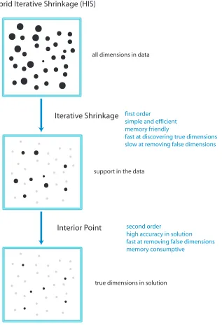
Hybrid Iterative Shrinkage (HIS)
Iterative Shrinkage
Interior Point
first order
simple and efficient memory friendly
fast at discovering true dimensions slow at removing false dimensions
second order
high accuracy in solution fast at removing false dimensions memory consumptive
all dimensions in data
support in the data
true dimensions in solution
There are several novel aspects of our hybrid approach. The rationale of the hybrid approach is based on the observation that the iterative shrinkage phase reduces the algorithm to gradient projection after a finite number of iterations, which will be described in Section 3.1. We build on this observation a hybrid approach to take advantage of the two phases of the computation using two types of numerical methods. In the first phase, inspired by the FPC by Hale et al. (2008), we customize the iterative shrinkage algorithm for the sparse logistic regression, whose objective function is not quadratic. In particular, the step length in the iterative shrinkage algorithm is not constant, unlike the compressive sensing problem. Therefore, we resort to a line search strategy to avoid computing the Hessian matrix (required for finding the step length for stability). In addition, theℓ1regularization is only applied to the w component and not v in sparse logistic regression. This change in the model requires a different shrinkage step, as well as a careful treatment in the line search strategy.
The remainder of the paper is organized as follows. In Section 2, we present the iterative shrink-age algorithm for sparse logistic regression, and prove its global convergence and Q-linear conver-gence. In Section 3, we provide the rationale for the hybrid approach, together with a description of the hybrid algorithm. Numerical results are presented in Section 4. We conclude the paper in Section 5.
2. Sparse Logistic Regression using Iterative Shrinkage
The iterative shrinkage algorithm used in the first phase is inspired by a fixed point continuation algorithm by Hale et al. (2008).
2.1 Notation
For simplicity, we define k · k:=k · k2, as the Euclidean norm. The support of x∈Rn is denoted by supp(x):={i : xi6=0}. We use g to denote the gradient of f , that is, g(x) =∇f(x),∀x. For any
index set I⊆ {1, . . . ,n}(later, we will use index sets E and L),|I|is the cardinality of I and xI is
defined as the sub-vector of x of length|I|, consisting only of components xi, i∈I. Similarly, for
any vector-value mapping h, hI(x)denotes the sub-vector of h(x)consisting of hi(x), i∈I.
To express the subdifferential ofk · k1we will use the signum function and multi-function (i.e., set-valued mapping). The signum function of t∈Ris
sgn(t):=
+1 t>0,
0 t=0,
−1 t<0;
while the signum multi-function of t∈Ris
SGN(t):=∂|t|=
{+1} t>0,
[−1,1] t=0,
{−1} t<0,
which is also the subdifferential of|t|.
For x∈Rn, we define sgn(x)∈Rn and SGN(x)⊂Rncomponent-wise as(sgn(x))i:=sgn(xi)
and max{x,y}are defined to operate component-wise, analogous with the definitions of sgn and SGN above. For x,y∈Rn, let x⊙y∈Rn denote the component-wise product of x and y, that is,
(x⊙y)i=xiyi. Finally, we let X∗denote the set of all optimal solutions of problem (3).
2.2 Review of Fixed Point Continuation forℓ1-minimization
A fixed-point continuation algorithm was proposed in Hale et al. (2008) as a fast algorithm for large-scale ℓ1-regularized convex optimization problems. The authors considered the following large-scaleℓ1-regularized minimization problem,
min
x∈Rn f(x) +λkxk1, (3)
where f :Rn→Ris differentiable and convex, but not necessarily strictly convex, andλ>0. They devised a fixed-point iterative algorithm and proved its global convergence, including finite con-vergence for some quantities, and a Q-linear (Quotient-linear) concon-vergence rate without assuming strict convexity of f or solution uniqueness. Numerically they demonstrated Q-linear convergence in the quadratic case f(x) =kAx−bk2
2, where A is completely dense, and applied their algorithm toℓ1-regularized compressed sensing problems. As we will adopt this algorithm for solving our problem (1), we review some important and useful results here and develop some new insights in the context ofℓ1-regularized logistic regression.
The rationale for FPC is based on the idea of operator splitting. It is well-known in convex analysis that minimizing a function in the form of φ(x) =φ1(x) +φ2(x), where both φ1 and φ2 are convex, is equivalent to finding a zero of the subdifferential∂φ(x), that is, seeking x satisfying
0∈T1(x) +T2(x)for T1:=∂φ1and T2:=∂φ2. We say(I+τT1)is invertible if y=x+τT1(x)has a unique solution x for any given y. Forτ>0, if(I+τT1)is invertible and T2is single-valued, then
0∈T1(x) +T2(x) ⇐⇒ 0∈(x+τT1(x))−(x−τT2(x)) ⇐⇒ (I−τT2)x∈(I+τT1)x
⇐⇒ x= (I+τT1)−1(I−τT2)x. (4) This gives rise to the forward-backward splitting algorithm in the form of a fixed-point iteration,
xk+1:= (I+τT1)−1(I−τT2)xk. (5) Applying (4) to problem (1), whereφ1(x):=λkxk1andφ2(x):= f(x), the authors of Hale et al. (2008) obtained the following optimality condition of x∗:
x∗∈X∗ ⇐⇒ 0∈g(x∗) +λSGN(x∗)⇐⇒x∗= (I+τT1)−1(I−τT2)x∗,
where T2(·) =g(·), the gradient of f(·), and(I+τT1)−1(·)is the shrinkage operator. Therefore, the fixed-point iteration (5) for solving (3) becomes
xk+1=s◦h(xk),
which is a composition of two mappings s and h fromRntoRn.
The gradient descent operator is defined as
The shrinkage operator, on the other hand, can be written as
s(·) =sgn(·)⊙max{| · | −ν,0}, (6)
whereν=λτ. Shrinkage is also referred to soft-thresholding in the language of wavelet analysis:
(s(y))i=
yi−ν, yi>ν,
0, yi∈[−ν,ν], yi+ν, yi<−ν.
In each iteration, the gradient descent step h reduces f(x)by moving along the negative gradient direction of f(xk)and the shrinkage step s reduces theℓ1-norm by “shrinking” the magnitude of each nonzero component in the input vector.
2.3 Iterative Shrinkage for Sparse Logistic Regression
Recall that in the sparse logistic regression problem (1), theℓ1regularization is only applied to w, not to v. Therefore, we propose a slightly different fixed point iteration. For simplicity of notation, we define column vectors u= (w; v)∈Rn+1and c
i= (ai; bi)∈Rn+1, where ai=bxi, for i=1,2, ...,m.
This reduces (1) to
min
u lavg(u) +λku1:nk1,
where lavg=m1∑mi=1θ(cTi u), andθdenotes the logistic transfer functionθ(z) =log(1+exp(−z)). The gradient and Hessian of lavgwith respect to u is given by
g(u) ≡ ∇lavg(u) = 1
m m
∑
i=1θ′(c⊤ i u)ci,
H(u) ≡ ∇2l
avg(u) = 1
m m
∑
i=1θ′′(c⊤ i u)cic⊤i ,
whereθ′(z) =−(1+ez)−1andθ′′(z) = (2+e−z+ez)−1. To guarantee convergence, we require the step length be bounded by 2(maxuλmaxH(u))−1.
The iterative shrinkage algorithm for sparse logistic regression is
uk+1 = s◦h1:n(uk),for w component,
uk+1 = hn+1(uk), for v component, (7) which is a composition of two mappings h and s fromRntoRn, where the gradient operator is
h(·) =· −τg(·) =· −τ∇lavg(·).
While the authors in Hale et al. (2008) use a constant step length satisfying
0<τ<2/λmax{HEE(u): u∈Ω},
Algorithm 1 Fixed-Point Continuation Algorithm
Require: A = [c⊤1; c⊤2;· · ·; c⊤m] ∈ Rm×(n+1), u = (w; v) ∈ Rn+1, f(u) = m−1φ(Au), task: minulavg(u) +λkuk1
Initialize u0
while “not converge” do
Armijo-like line search algorithm (Algorithm 2)
k=k+1
end while
2.4 Convergence
Global convergence and finite convergence on certain quantities were proven in Hale et al. (2008) when the following conditions are met: (i) the optimal solution set X∗is non-empty, (ii) f ∈C2and its Hessian H=∇2f is positive semi-definite inΩ={x :kx−x∗k ≤ρ} ⊂Rnforρ>0, and (iii) the
maximum eigenvalue of H is bounded onΩby a constant ˆλmaxand the step lengthτis uniformly less than 2/λˆmax. These conditions are sufficient for the forward operator h(·)to be non-expansive.
Assumption 1 Assume problem (1) has an optimal solution set X∗6=/0, and there exists a set Ω={x :kx−x∗k ≤ρ} ⊂Rn
for some x∗∈X∗andρ>0 such that f ∈C2(Ω), H(x):=∇2f(x)0 for x∈Ωand ˆ
λmax:=sup
x∈Ω
λmax(H(x))<∞.
For simplicity for the analysis, we choose a constant step lengthτin the fixed-point iterations (7): xk+1=s(xk−τg(xk)), whereν=τλ, and
τ∈0,2/ˆλmax
,
which guarantees that h(·) =I(·)−τg(·)is non-expansive inΩ.
Theorem 1 Under Assumption, the sequence{uk}generated by the fixed-point iterations (7) ap-plied to problem (1) from any starting point x0∈Ωconverges to some u∗∈U∗∩Ω. In addition, for all but finitely many iterations, we have
uki =u∗i =0, ∀i∈L={i :|g∗i|<λ,1≤i≤n}, (8) sgn(hi(uk)) =sgn(hi(u∗)) =−1
λg∗i, ∀i∈E={i :|g∗i|=λ,1≤i≤n}, (9)
where as long as
ω:=min{ν(1−|g
∗ i|
λ ): i∈L}>0.
The numbers of iterations not satisfying (8) and (9) do not exceedku0−u∗k2/ω2andku0−u∗k2/ν2,
Proof We sketch the proof here. First, the iteration (7) is shown to be non-expansive inℓ2, that is, kuk−u∗k does not increase in k with the assumption on the step length τ. Specifically, in Assumption, the step lengthτis chosen small enough to guarantee thatkh(uk)−h(u∗)k ≤ kuk−u∗k (in practice,τis determined, for example, by line search.) On the other hand, through a component-wise analysis, one can show that no matter what τ is, the shrinkage operator s(·) is always non-expansive, that is,ks(h1:n(uk))−s(h1:n(u∗))k ≤ kh1:n(uk)−h1:n(u∗)k. Therefore, from the definition of uk+1in (7), we have
kuk+1−u∗k ≤ kuk−u∗k, (10) using the fact that u∗is optimal if and only if u∗is a fixed point with respect to (7). However, this non-expansiveness of (7) does not directly give convergence.
Next,{uk}is shown to have a limit point ¯x, that is, a subsequence converging to ¯u, due to the
compactness ofΩand (10). (7) can be proven to converge globally to ¯u. To show this, we first get
k[s◦h1:n(u¯); hn+1(u¯)]−[s◦h1:n(u∗); hn+1(u∗)]k=ku¯−u∗k,
from the fact that ¯u is a limit point, and then use this equation to show that ¯u= [s◦h1:n(u¯); hn+1(u¯)], that is, ¯u is a fixed point with respect to (7), and thus an optimal solution. Repeating the first step
above we havekuk+1−u¯k ≤ kuk−u¯k, which extends ¯u from being the limit of a subsequence to
one of the entire sequence.
Finally, to obtain the finite convergence result, we need to take a closer look at the shrinkage operator s(·). When (8) does not hold for some iteration k at component i, we have|uik+1−u∗i|2≤ |uki −u∗i|2−ω2, and for (9), we have|uk+1
i −u∗i|2≤ |uik−u∗i|2−ν2. Obviously, there can be only
a finite number of iterations k in which either (8) or (9) does not hold, and such numbers do not exceedku0−u∗k2/ω2andku0−u∗k2/ν2, respectively.
A linear convergence result with a certain convergence rate can also be obtained. As long as
HEE(x∗):= [Hi,j(x∗)]i,j∈Ehas full rank or f(x)is convex quadratic in x, the sequence{xk}converges
to x∗ R-linearly, and {kxkk1+µ f(xk)} converges to kx∗k1+µ f(x∗) Q-linearly. Furthermore, if
HEE(x∗)has the full rank, then R-linear convergence can be strengthened to Q-linear convergence by using the fact that the minimal eigenvalue of HEE at x∗is strictly greater than 0.
2.5 Line Search
An important element of the iterative shrinkage algorithm is the step lengthτat each iteration. To ensure the stability of the algorithm, we require that the step length satisfy
0<τ<2/λmax{HEE(u): u∈Ω}.
Algorithm 2 Armijo-like Line Search Algorithm
Compute heuristic step lengthα0 Gradient step: uk−=uk−α0∇lavg(uk) Shrinkage step: uk+=s1:n(uk−,λα0) Obtain search direction: pk=uk+−uk while “j<max line search attempts” do
if Armijo-like condition is met then
Accept line search step, update uk+1=uk+αjpk else
Keep backtrackingαj=µαj−1
end if j= j+1
end while
Let’s denote the objective function for theℓ1-regularized logistic regression asφ(u)for conve-nience:
φ(u) =lavg(u) +λku1:nk1, where lavg(u) = 1
m∑ m
i=1θ(cTi u)andθis the logistic transfer function. A line search method, at each
iteration, computes the step lengthαk and the search direction pk:
uk+1=uk+αkpk.
The search direction will be described in Eqn. (12). For our sparse logistic regression, a sequence of step length candidates are identified, and a decision is made to accept one when certain conditions are satisfied. We compute a heuristic step length and gradually decrease it until a sufficient decrease condition is met.
Let’s define the heuristic step length as α0. Ideally the choice of step length α0, would be a global minimizer of the smooth part of the objective function,
ϕ(α) =lavg(uk+αpk), α>0,
which is too expensive to evaluate, unlike the quadratic case in compressive sensing. Therefore, an inexact line search strategy is usually performed in practice to identify a step length that achieves sufficient decrease inϕ(α)at minimal cost. Motivated by a similar approach in GPSR (Figueiredo et al., 2007), we compute the heuristic step length through a minimizer of the quadratic approxima-tion forϕ(α),
lavg(uk−α∇lavg(uk))≈lavg(uk)−α∇lavg(uk)T∇lavg(uk) +0.5α2∇lavg(uk)TH(uk)∇lavg(uk). Differentiating the right-hand side with respect toαand setting the derivative to zero, we obtain
α0=
∇lavg(u¯k)T∇lavg(u¯k)
∇lavg(u¯k)TH(u¯k)∇lavg(u¯k)
, (11)
Based on the heuristic step lengthα0, we can obtain the search direction pk, which is a combi-nation of the gradient descent step and the shrinkage step:
uk−=uk−α0∇lavg(uk),
uk+=s1:n(uk−,λα0),
pk=uk+−uk. (12)
It is easy to verify that sν(y) is the solution to the non-smooth unconstrained minimization problem min12kx−yk2
2+λkxk1. This minimization problem is equivalent to the following smooth constrained optimization problem,
min1 2kx−yk
2
2+νz, subject to(x,z)∈Ω:={(x,z)| kxk1≤z}, whose optimality condition is
(s(x,ν)−x)T(y−s(x,ν) +ν(z− ks(x,ν)k1)≥0,
for all x∈Rn,(y,z)∈Ωandν>0. Once we substitute u−τg for x, u for y,ku1:nk1for z and set
ν=λτ, the optimality condition becomes
(s1:n(u−τg,λτ)−(u−τg))T(u−s1:n(u−τg,λτ)) +λτ(ku1:nk1− ks1:n(u−τg,λτ)k1)≥0.
Using the fact u+=s1:n(u−τg,λτ), p=u+−u, we get
gTp+λ(ku+1:nk1− ku1:nk1)≤ −pTp/τ, which means
∇lavg(uk)
T
pk+λkuk1:n+k1−λkuk1:nk1≤0.
We then geometrically backtrack the step lengths, letting αj =α0, µα0, µ2α0, . . ., until the following Armijo-like condition is satisfied:
φ(uk+αjpk)≤Ck+αj∆k.
Notice that the Armijo-like condition for line search stipulates that the step lengthαj in the search
direction pk should produce a sufficient decrease of the objective functionφ(u). Ck is a reference
value with respect to the previous objective values, while the decrease in the objective function is described as
∆k:=∇lavg(uk)
T
pk+λkuk1:n+k1−λkuk1:nk1≤0.
There are two types of Armijo-like conditions depending on the choice of Ck. One can choose Ck =φ(uk), which makes the line search monotone. One can also derive a non-monotone line search, where Ckis a convex combination of the previous value Ck−1and the function valueφ(uk). We refer interested readers to Wen et al. (2009) for more details.
2.6 Continuation Path
A continuation strategy is adopted in our algorithm, by designing a regularization path similar to that is used in Hale et al. (2008),
λ0>λ1> ... >λL−1=¯λ.
This idea is closely related to the homotopy algorithm in statistics, and has been successfully applied to theℓ1-regularized quadratic case, where the fidelity term is f(x) =kAx−bk2
2. The ratio-nale of using such a continuation strategy is due to a fast rate of convergence for largeλ. Therefore, by taking advantage of different convergence rate for a family of regularization parameter λ, if stopped appropriately, we can speed up the convergence rate of the full path. An intriguing discus-sion regarding the convergence rate of fixed-point algorithm withλandω, the spectral properties of Hessian, was presented in Hale et al. (2008). In the case of the logistic regression, we have decided to use the geometric progression for the continuation path. We define
λi=λ0βi−1,for i=0, ...,L−1,
whereλ0can be calculated based on the ultimate ¯λwe are interested in and the continuation path length L, that is,λ0=¯λ/βL−1.
As mentioned earlier, the goal of a continuation strategy is to construct a path with different rate of convergence, with which we can speed up the whole algorithm. The solution obtained from a previous subpath associated withλi−1is used as the initial condition for the next subpath forλi.
Note that we design the path length L and the geometric progression rateβin such a way that the initial regularizationλ0is fairly large, leading to a sparse solution for the initial path. Therefore, the initial condition for the whole path, considering the sparsity in solution, is a zero vector.
Another design issue regarding such a continuation strategy is we stop each subpath according to some criteria, in an endeavor to approximate the solution in the nextλas fast as possible. This means that a strong convergence is not required in subpath’s except for the final one, and we can vary the stopping criteria to “tighten” such a convergence as we proceed. The following two stopping criteria are used:
kuk+1−ukk
max(kukk,1) <utoli,
k∇lavg(uk)k∞
λi
−1<gtol.
The first stopping criterion requires that relative change in u be small, while the second one is related to the optimality condition, defined in Eqn. (13). Theoretically, we would like to vary utolito attain
a seamless Q-linear convergence path. Such a choice seems to be problem dependent, and probably even data dependent in practice. It remains an important, yet difficult research topic to study the properties of different continuation strategies. We have chosen to use a geometric progression for the tolerance value, utoli=utol0∗γi−1, with utol0=utol/γL−1. In our numerical simulation, we use utol=10−4and gtol=0.2.
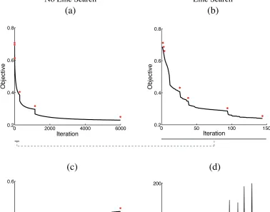
fairly flat reduction at earlier stages of the path. Clearly by relaxing the convergence at earlier stages of the path, we can accelerate the computation, shown in (b). The choice of utol and gtol seems to be data dependent in our experience, and the result we show in (b) might be suboptimal. Further optimization of the continuation path can potentially accelerate the computation even more, which remains an open question for future research.
0 100 200 300 400 500
0.2 0.4 0.6 0.8
Iteration
Objective
0 50 100 150 200
0.2 0.4 0.6 0.8
Iteration
Objective
(a) Fix
utol
(b) Vary
utol
Figure 3: Illustration of the continuation strategy (a) using a fixed utol =0.0001 is used for the stopping criterion, (b) using a varying utol according to geometric progression. Note that a stronger convergence is not necessary in earlier stages on the continuation path. By using a varying utol, especially tightening utol as we move along the path, we can accelerate the fixed point continuation algorithm. Shown is the objective value (black curve) as a function of iteration, where the transition point on the regularization path is labeled in (red asterisk). Data used in this experiment has 10000 dimension and 100 samples. A continuation path of length 8, starting from 0.128 and ending at 0.001.
3. Hybrid Iterative Shrinkage (HIS) Algorithm
In this section we describe a hybrid approach called HIS, which uses the iterative shrinkage algo-rithm described previously to enforce sparsity and identify the support in the data, followed by a subspace optimization via an interior point method.
3.1 Why A Hybrid Approach?
The hybrid approach is based on an interesting observation for the iterative shrinkage algorithm, regarding some finite convergence properties. The optimality condition for min f(x) +λkxk1is the following
which requires that|gi| ≤λ, for i=1, ...,n. We define two index sets
L :={i :|g∗i|<λ} and E :={i :|g∗i|=λ},
where g∗=g(u∗)is constant for all u∗∈X∗ and|g∗i| ≤λfor all i. Hence, L∩E=/0 and L∪E=
{1, . . . ,n}. The following holds true for all but a finite number of k:
uki =u∗i =0, ∀i∈L,
sgn(hi(uk)) =sgn(hi(u∗)) =−
1
λg∗i, ∀i∈E.
Assume that the underlying problem is nondegenerate, then L and E equal the sets of zero and nonzero components in x∗. According to the above finite convergence result, the iterative shrinkage algorithm obtains L and E, and thus the optimal support and signs of the optimal nonzero compo-nents, in a finite number of steps.
Corollary 2 Under Assumption 1, after a finite number of iterations, the fixed-point iteration (7) reduces to gradient projection iterations for minimizingφ(uE)over a constraint set OE, where
φ(uE):=−(g∗E)⊤uE+f((uE; 0)),and
OE={uE ∈R|E|:−sgn(g∗E)⊙uE ≥0}. Specifically, we have uk+1= (ukE+1; 0)in which
ukE+1:=POE
ukE−τ∇φ(ukE),
where POE is the orthogonal projection onto OE, and∇φ(uE) =−g ∗
E+gE((uE; 0)).
This corollary, see Corollary 4.6 in Hale et al. (2008), can be directly applied to sparse logistic regression. The fixed point continuation reduces to the gradient projection after a finite number of iterations. The proof of this corollary is in general true for the u1:n, that is, the w component in our problem.
Corollary 2 implies an important fact: there are two phases in the fixed point continuation algorithm. In the first phase, the number of nonzero elements in the x evolve rapidly, until after a finite number of iterations, when the support (non-zero elements in a vector) is found. Precisely, it means that for all k>K, the nonzero entries in uk include all true nonzero entries in u∗ with the matched signs. However, unless k is large, uk typically also has extra nonzeros. At this point, the fixed point continuation reduces to the gradient projection, starting the second phase of the algorithm. In the second phase, the zero elements in the vector stay unaltered, while the magnitude of the nonzero elements (support) keeps evolving.
The above observation is a general statement for any f that is convex. Recall the quadratic case, where f =ky−Axk2
regularization parameter ¯λof interest. In some sense, we have designed a continuation path that is super-fast until it reaches the second phase of the final subpath. This is not surprising given that the fixed point continuation algorithm is based on gradient descent and shrinkage operator. We envision that by switching to a Newton’s method, we can accelerate the second phase.
Based on this intuition, we are now in a position to describe a hybrid algorithm: a fixed point continuation plus an interior point truncated Newton method. For the latter part we resort to the customized interior point in Koh et al. (2007). We modified the source code of the l1logreg software (written in C), and built an interface to our MATLAB code. This hybrid approach, based on our observation of the two phases, enables us to attain a good balance of speed and accuracy.
3.2 Interior Point Phase
The second phase of our HIS algorithm used an interior point method developed by Koh et al. (2007). We directly used a well-developed software package l1logreg1 and modified the source code to build an interface to MATLAB. We review some key points for the interior point method here.
In Koh et al. (2007), the authors overcome the difficulty of non-differentiability of the objec-tive function by transforming the original problem into an equivalent one with linear inequality constraints,
min 1
m m
∑
i=1lavg(wTai+vbi) +λ1Tu s.t. −ui≤wi≤ui, i=1, ...,n.
A logarithmic barrier function, smooth and convex, is further constructed for the bound con-straints,
ρ(w,u) =−
n
∑
i=1log(ui+wi)− n
∑
i=1log(ui−wi),
defined on the domain{(w,u)∈Rn×Rn||wi|<ui,i=1, ...,n}. The following optimization problem
can be obtained by augmenting the logarithmic barrier,
ψt(v,w,u) =tlavg(v,w) +tλ1Tu+ρ(w,u),
where t >0. The resulting objective function is smooth, strictly convex and bounded below, and therefore has a unique minimizer(v∗(t),w∗(t),u∗(t)). This defines a curve inR×Rn×Rn,
param-eterized by t, called the central path. The optimal solution is also shown to be dual feasible. In addition,(v∗(t),w∗(t))is 2n/t-suboptimal.
As a primal interior-point method, the authors computed a sequence of points on the central path, for an increasing sequence of values of t, and minimized ψt(v,w,u) for each t using a truncated
Newton’s method. The interior point method was customized by the authors in several ways: 1) the dual feasible point and the associated duality gap was computed in a cheap fashion, 2) the central path parameter t was updated to achieve a robust convergence when combined with the preconditioned conjugate gradient (PCG) algorithm, 3) an option for solving the Newton’s system was given for problems of different scales, where small and medium dense problems were solved by direct methods (Cholesky factorization), while large problems were solved using iterative methods (conjugate gradients). Interested readers are referred to Koh et al. (2007) for more details.
3.3 The Hybrid Algorithm
The hybrid algorithm leverages the computational strengths of both the iterative shrinkage solver and the interior point solver.
Algorithm 3 Hybrid Iterative Shrinkage (HIS) Algorithm
Require: A= [c⊤1; c⊤2;· · ·; c⊤m]∈Rm×n+1, u= (w; v)∈Rn+1, f(u) =m−1φ(Au)
task: minulavg(u) +λkuk1 Initialize u0
PHASE 1 : ITERATIVE SHRINKAGE
Selectλ0and utol0
while “not converge” do
if “the last continuation path”, i== (L−1)and “transition condition” then “transit into PHASE 2”
else
Updateλi=λi−1β, utoli=utoli−1γ Compute heuristic step lengthα0
Gradient descent step: uk−=uk−α0∇lavg(uk) Shrinkage step: uk+=s1:n(uk−,λα0)
Obtain line search direction: pk=uk+−uk while “j<max line search attempts” do
if Armijo-like condition is met then
Accept line search step, update uk+1=uk+αjpk else
Keep backtrackingαj=µαj−1
end if j=j+1
end while end if end while
PHASE 2 : INTERIOR POINT
Initialize ˜w=wnonzero get subproblem minψt(v,w,u˜ ) while “not converged”η>εdo
Solve the Newton system :∇2ψkt(v,w,˜ u)[∆v,∆w,˜ ∆u] =−∇ψk
t(v,w,u˜ )
Backtracking line search : find the smallest integer j≥0 that satisfies
ψk
t(v+αj∆v,w˜+αj∆w,˜ u+αj∆u)≤ψkt(v,w,˜ u) +cαj∇ψkt(v,w,u˜ )T[∆v,∆w,˜ ∆u]
Updateψkt+1(v,w,˜ u) =ψk
t(v,w,u˜ ) +αj(∆v,∆w,˜ ∆u)
Check dual feasibility Evaluate duality gapη
k=k+1
end while
last subpath whereλis the desired one, we transit to the interior point when the true support of the vector is found. The corollary in Section 3.1 states that iterative shrinkage recovers the true support in a finite number of steps. In addition, iterative shrinkage obtains all true nonzero components long before the true support is obtained. Therefore, as long as the iterative shrinkage seems to stagnate, which can be observed when the objective function evolves very slowly, it is highly likely that all true nonzero components are obtained. This indicates that the algorithm is ready for switching to the interior point.
In practice, we require the following transition condition,
kuk+1−ukk
max(kukk,1) <utolt,
and extract the nonzero components in w as the input to the interior point solver. By doing so, we reduce the problem to a subproblem where the dimension is much smaller, and solve the subproblem using the interior point method.
The resulting hybrid algorithm achieves high computational speed while attaining the same numerical accuracy as the interior point method, as demonstrated with empirical results in the next section.
4. Numerical Results
In this section we present numerical results, on a variety of data sets, to demonstrate the benefits of our hybrid framework in terms of computational efficiency and accuracy.
4.1 Benchmark
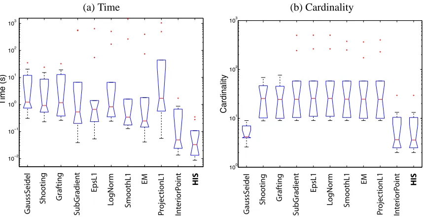
We carried out a numerical comparison of the HIS algorithm with several existing algorithms in liter-ature forℓ1-regularized logistic regression. Inspired by a comparison study on this topic by Schmidt et al. (2007),2 we compared our algorithm with 10 algorithms, including a generalized version of Gauss-Seidel, Shooting, Grafting, Sub-Gradient, epsL1, Log-Barrier, Log-Norm, SmoothL1, EM, ProjectionL1 and Interior-Point method. In the numerical study, we replaced the interior point solver by the one written by Koh et al. (2007). Benchmark data were taken from the publicly avail-able UCI machine learning repository.3 We used 10 data sets of small to median size (internetad1, arrhythmia, glass, horsecolic, indiandiabetes, internetad2, ionosphere, madelon, pageblock, spam-base, spectheart, wine).
All of the methods were run until the same convergence criteria was met, where appropriate, for instance the step length, change in function value, negative directional derivative, optimality condition, convergence tolerance is less than 10−6. We treated each algorithm solver as a black box and evaluated both the computation time and the sparsity (measured by cardinality of solution). We set an upper limit of 250 iterations, meaning we stop the solver when the number of iteration exceeds 250. Since different algorithm has different speed for each iterate (usually a Newton step is more expensive than a gradient descent step), we think the computation time is a more appropriate evaluation criterion than number of iterations. The ability of the algorithm to find a sparse solution, measured by the cardinality, was also evaluated in this process.
2. Source code is available athttp://www.cs.wisc.edu/˜gfung/GeneralL1.
Figure 4 shows the benchmark result using data from the UCI machine learning repository. All numerical results shown are averaged over a regularization path. The parameters for the regulariza-tion path are calculated according to each data set, where the maximal regularizaregulariza-tion parameter is calculated as follows:
λmax=
1
m
m− m b
∑
i=+1 ai+
m+
m b
∑
i=−1ai
∞, (14)
where m−is the number of training samples with label−1 and m+is the number of training samples with label +1 (Koh et al., 2007). λmax is an upper bound for the useful range of regularization
parameter. When λ≥λmax, the cardinality of the solution will be zero. In this case, we test a
regularization path of length 10, that is,λmax, 0.9λmax, 0.8λmax... 0.1λmax. Among all the numerical
solvers, our HIS algorithm is the most efficient. HIS achieves comparable cardinality in the solution, compared to the interior point solver.
We also evaluated the accuracy of the solution by looking at the classification performance using Kfold cross-validation. Table 1 summaries the accuracy of the solution using the HIS algorithm, compared to the interior point (IP) algorithm. Clearly, HIS algorithm achieves comparable accuracy compared to IP, an algorithm that is recognized for its high accuracy.
(a) Time (b) Cardinality
10−2 10−1 100 101 102 103 Time (s) G aussS eidel S h o o ti n g G ra ft in g S u b G ra d ie n t E p sL 1 Lo g N o rm SmoothL1 EM P rojec tionL1 In ter io rP o in t HIS 100 101 102 103 C a rd in a lit y G aussS eidel S h o o ti n g G ra ft in g S u b G ra d ie n t E p sL 1 Lo g N o rm SmoothL1 EM P rojec tionL1 In ter io rP o in t HIS
Figure 4: Comparison of our hybrid iterative shrinkage (HIS) method with several other existing methods in literature. Benchmark data were taken from the UCI machine learning reposi-tory, including 10 publicly available data sets. (a) Distribution of computation time across 10 data sets, (b) Distribution of cardinality for the solution across 10 data sets, averaged over a regularization path.
4.2 Scaling Result
Accuracy Comparison (Az∈[0.5,1.0])
dataname accuracy(HIS) accuarcy(IP)
arrhythmia 0.7363 0.7363
glass 0.6102 0.6102
horsecolic 0.5252 0.5252
ionosphere 0.5756 0.5756
madelon 0.6254 0.6254
spectheart 0.5350 0.5350
wine 0.6102 0.6102
internetad 0.8486 0.8486
Table 1: Comparison of solution accuracy for our hybrid iterative shrinkage (HIS) algorithm and the interior point (IP) algorithm. Accuracy of the solution was measured by Az value, resulted from Kfold cross-validation, where Kfold is 10. A regularization path of varying
λwere computed to determine the maximum generalized Az value. The data sets were taken from the UCI machine learning repository.
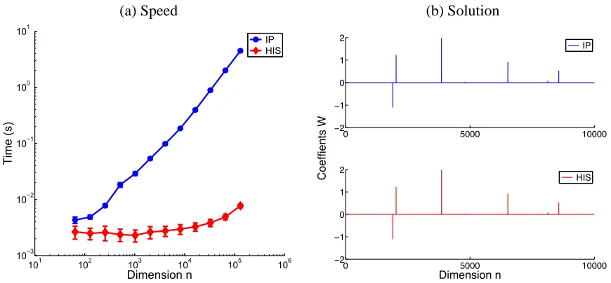
data is drawn from a Normal distribution, where the mean of the distribution is shifted by a small amount for each class (0.1 for samples with label 1, and −0.1 for samples with label−1). The number of samples is the same for both classes and chosen to be smaller than the dimension of the data. Experiments for each dimension were carried out on 100 different sets of random data. We compared the mean and variances of the computation time, and compared our HIS algorithm to the IP algorithm.
Table 2 summarizes the computational speed for the HIS algorithm and the IP algorithm. It is noteworthy that the HIS algorithm improves the efficiency of computation, while maintaining comparable accuracy to the IP algorithm. Figure 5 plots the computation result as a function of dimension for better illustration. In (a) one can clearly see the speedup we gain from the HIS algorithm (red), compared to the IP algorithm (blue). We also show the solution quality in (b), where the weights we get from both solvers, is comparable.
4.3 Regularization Parameter
In general, the regularization parameterλaffects the number of iterations to converge for any solver. Asλbecomes smaller, the cardinality of the solution increases, and the computation time needed for convergence also increases. Therefore when one seeks a solution with less sparsity (smallλ), it is more computationally expensive.
In practice, when one carries out classification on a set of data, the optimal regularization pa-rameter is often unknown. Speaking of optimality, we refer to a regularization papa-rameter that results in the best classification result evaluated using Kfold cross-validation. One would run the algorithm along a regularization path,λmax, ...,λmin, whereλmax is computed by Eqn. (14) and whereλminis
supplied by the user.
Speed Comparison (in second)
dimension mean(HIS) std(HIS) mean(IP) std(IP)
64 0.0026 0.00069 0.0043 0.00057
128 0.0025 0.00058 0.0049 0.00037 256 0.0026 0.00075 0.0078 0.00052
512 0.0024 0.00059 0.018 0.0017
1024 0.0023 0.00056 0.029 0.0023
2048 0.0026 0.00064 0.054 0.0026
4096 0.0028 0.00057 0.098 0.0050
8192 0.0030 0.00059 0.19 0.0076
16384 0.0033 0.00055 0.40 0.018
32768 0.0038 0.00055 0.89 0.037
65536 0.0049 0.00054 2.01 0.096
131072 0.0077 0.00056 4.49 0.24
Table 2: Speed comparison of the HIS algorithm with the IP algorithm, based on simulated random benchmark data. Shown here is the computation speed as a function of dimension. Data used here are generated by sampling from two Gaussian distributions. Note that in the simulation, the continuation path used in the iterative shrinkage may or may not be optimal, which means that the speed profile for the HIS algorithm can be essentially accelerated even more.
(a) Speed (b) Solution
101 102 103 104 105 106
10−3 10−2 10−1 100 101
Dimension n
T
ime
(s)
IP HIS
0 5000 10000
−2 −1 0 1 2
0 5000 10000
−2 −1 0 1 2
Dimension n
Coeffients W
IP
HIS
λ
W
0 0.05 0.1
0.15 0.2
5
10
15
20
25
30
−4 −2 0 2 4 6 8
Figure 6: Solution w evolves along a regularization path, following a geometric progression from 10−1 to 10−4. Data is ionosphere from UCI machine learning repository. As theλ be-comes smaller, the cardinality of the solution goes up.
in the solution, and one can determine the optimal sparsity for the data. This is an attractive prop-erty of this model, where one can search in the feature space the most informative features about discrimination.
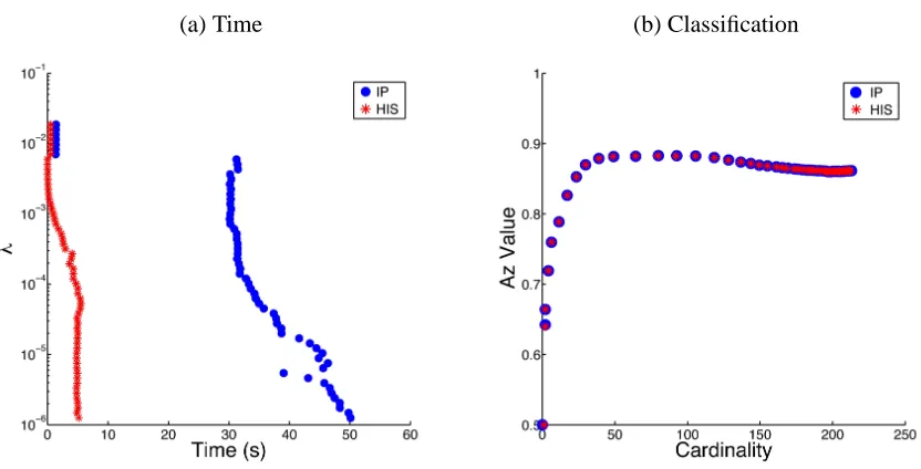
We illustrate the effect of the regularization parameter using real data of large scale. The data concerns a two alternative force choice task for face versus car discrimination. We used a spik-ing neuron model of primary visual cortex to map the input into cortical space, and decoded the resulting spike trains using sparse logistic regression (Shi et al., 2009). The data has 40960 dimen-sions and 360 samples for each of the two classes. Kfold cross-validation was used to evaluate the classification performance, where the number of Kfolds is 10 in our simulation.
(a) Time (b) Classification
Figure 7: An example using real data of large scale, n=40960, m=360. (a) Computation time along such a regularization path, where the smallerλrequires more computation time. Note that the simulation is carried out for eachλ separately. (b) Classification perfor-mance derived from ROC analysis based on Kfold cross-validation. Data used in this simulation are neural data for a visual discrimination task (Shi et al., 2009).
4.4 Data Sets with Large Dimensions and Samples
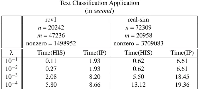
We applied the HIS algorithm to some examples of real-world data that have both large dimensions
n and samples m. In this case, we considered text classification using the binary rcv1 data4(Lewis et al., 2004), and real-sim data.5
We ran the simulation on an Apple Mac Pro with two 3 GHz Quad-Core Intel processors, and 8 GB of memory. The timing of the simulation was calculated within the Matlab interface. All the operations were optimized for sparse matrix computation. Table 3 summarizes the numerical results. For both examples of text classification, we observed a speedup using the HIS algorithm while attaining the same numerical accuracy, compared with the IP algorithm. The regularization parameter does affect the computational efficiency, as we have observed in the previous section.
5. Conclusion
We have presented in this paper a computationally efficient algorithm for theℓ1-regularized logistic regression, also called the sparse logistic regression. The sparse logistic regression is a widely used model for binary classification in supervised learning. The ℓ1 regularization leads to sparsity in the solution, making it a robust classifier for data whose dimensions are larger than the number of
4. Binary rcv1 data is available athttp://www.csie.ntu.edu.tw/˜cjlin/libsvmtools/datasets/binary.html#
rcv1.binary.
Text Classification Application (in second)
rcv1 real-sim
n = 20242 n = 72309
m = 47236 m = 20958
nonzero = 1498952 nonzero = 3709083
λ Time(HIS) Time(IP) Time(HIS) Time(IP)
10−1 0.11 1.93 0.62 6.61
10−2 0.27 1.93 0.62 6.61
10−3 2.08 8.20 5.50 18.45
10−4 5.80 8.66 13.12 19.36
Table 3: Illustration of performance on text classification, where both the dimensions n and samples
m are large-scale. We compare the computational efficiency of the HIS and IP algorithms.
In both cases, the solution accuracy is the same.
samples. Sparsity also provides an attractive avenue for feature selection, useful for various data mining tasks.
Solving the large-scale sparse logistic regression usually requires expensive computational re-sources, depending on the specific solver, memory and/or CPU time. The interior point method is so far the most efficient solver in the literature, but requires expensive memory consumption. We have presented the HIS algorithm, which couples a fast shrinkage method and a slower but more accurate interior point method. The iterative shrinkage algorithm has global convergence with a Q-linear rate. Various techniques such as line search and continuation strategy are used to accelerate the computation. The shrinkage solver only involves the gradient descent and the shrinkage operator, both of which are first-order. Based solely on efficient memory operations such as matrix-vector multiplication, the shrinkage solver serves as the first phase for the algorithm. This reduces the problem to a subspace whose dimension is smaller than the original problem. The HIS algorithm then transits into the second phase, using a more accurate interior point solver. We numerically compare the HIS algorithm with other popular algorithms in the literature, using benchmark data from the UCI machine learning repository. We show that the HIS algorithm is the most computa-tionally efficient, while maintaining high accuracy. The HIS algorithm also scales very well with dimension of the problem, making it attractive for solving large-scale problems.
There are several ways to extend the HIS algorithm. One is to extend it beyond binary classifi-cation, allowing for multiple classes (Krishnapuram and Hartemink, 2005). The other is to further improve the regularization path. When applying the HIS algorithm, one will usually explore a range of sparsity by constructing a regularization path (λmax, λ1, ..., λmin). Usually the smaller the λ,
Acknowledgments
We thank Mads Dyrholm (Columbia University) for fruitful discussions. We appreciate the anony-mous reviewers, who have helped improve the quality of our paper. Jianing Shi and Paul Sajda’s work was supported by grants from NGA (HM1582-07-1-2002) and NIH (EY015520). Wotao Yin’s work was supported by NSF CAREER Award DMS-0748839 and ONR Grant N00014-08-1-1101. Stanley Osher’s work was supported by NSF grants DMS-0312222, and ACI-0321917 and NIH G54 RR021813.
References
C.M. Bishop. Pattern Recognition and Machine Learning. Springer, 2007.
S. Boyd, S.-J. Kim, L. Vandenberghe, and A. Hassibi. A tutorial on geometric programming.
Opti-mization and Engineering, 8(1):67–127, 2007.
M. Burger, G. Gilboa, S. Osher, and J. Xu. Nonlinear inverse scale space methods. Communications
in Mathematical Sciences, 4:179–212, 2006.
E.J. Cand´es and T. Tao. Near optimal signal recovery from random projections: Universal encoding strategies? IEEE Trans. Inform. Theory, 52(2):5406–5425, 2006.
E.J. Cand´es, J. Romberg, and T. Tao. Robust uncertainty principles: Exact signal reconstruction from highly incomplete frequency information. IEEE Trans. Inform. Theory, 52(2):489–509, 2006.
S. Chen, D.L. Donoho, and M.A. Saunders. Atomic decomposition by basis pursuit. SIAM J.
Scientific Computing, 20:33–61, 1998.
J.F. Claerbout and F. Muir. Robust modeling with erratic data. Geophysics, 38(5):826–844, 1973.
A. d’Aspremont, L. El Ghaoui, M. Jordan, and G. Lanckriet. A direct formulation for sparse pca using semidefinite programming. In Advances in Neural Information Processing Systems, pages 41–48. MIT Press, 2005.
D.L. Donoho. Compressed sensing. IEEE Trans. Inform. Theory, 52:1289–1306, 2006.
D.L. Donoho and M. Elad. Optimally sparse representations in general nonorthogonal dictionaries byℓ1minimization. Proc. Nat’l Academy of Science, 100(5):2197–2202, 2003.
D.L. Donoho and X. Huo. Uncertainty principles and ideal atomic decomposition. IEEE. Trans.
Inform. Theory, 48(9):2845–2862, 2001.
D.L. Donoho and B.F. Logan. Signal recovery and the large sieve. SIAM J. Appl. Math., 52(2): 577–591, 1992.
D.L. Donoho, I. Johnstone, G. Kerkyacharian, and D. Picard. Wavelet shrinkage: Asymptopia? J.
Roy. Stat. Soc. B, 57(2):301–337, 1995.
B. Efron, T. Hastie, I. Johnstone, and R. Tibshirani. Least angle regression. Annals of Statistics, 32(2):407–499, 2004.
S. Eyheramendy, A. Genkin, W. Ju, D. Lewis, and D. Madigan. Sparse bayesian classifiers for text categorization. Technical report, J. Intelligence Community Research and Development, 2003.
M. Figueiredo. Adaptive sparseness for supervised learning. IEEE Trans. Pattern Analysis and
Machine Intelligence, 25:1150–1159, 2003.
M. Figueiredo and A. Jain. Bayesian learning of sparse classifiers. In IEEE Conf. Computer Vision
and Pattern Recognition, pages 35–41, 2001.
M. Figueiredo, R. Nowak, and S. Wright. Gradient projection for sparse reconstruction: application to compressed sensing and other inverse problems. IEEE J. Selected Topics in Signal Processing:
Special Issue on Convex Optimization Methods for Signal Processing, 1(4):586–598, 2007.
A. Genkin, D.D. Lewis, and D. Madigan. Large-scale bayesian logistic regression for text catego-rization. Technometrics, 49(3):291–304, 2007.
A.D. Gerson, L.C. Parra, and P. Sajda. Cortical origins of response time variability during rapid discrimination of visual objects. Neuroimage, 28(2):342–353, 2005.
A. Ghosh and S. Boyd. Growing well-connected graphs. In 45th IEEE Conference on Decision and
Control, pages 6605–6611, 2006.
J. Goodman. Exponential priors for maximum entropy models. In Proceedings of the Annual
Meetings of the Association for Computational Linguistics, 2004.
E. Hale, W. Yin, and Y. Zhang. Fixed-point continuation forℓ1-minimization: methodology and convergence. SIAM J. Optimization, 19(3):1107–1130, 2008.
A. Hassibi, J. How, and S. Boyd. Low-authority controller design via convex optimization. AIAA
Journal of Guidance, Control and Dynamics, 22(6):862–872, 1999.
K. Koh, S.-J. Kim, and S. Boyd. An interior-point method for large-scaleℓ1-regularized logistic regression. J. Machine Learning Research, 8:1519–1555, 2007.
B. Krishnapuram and A. Hartemink. Sparse multinomial logistic regression: fast algorithms and generalization bounds. IEEE Trans. Pattern Analysis and Machine Intelligence, 27(6):957–968, 2005.
B. Krishnapuram, L. Carin, and M. Figueiredo. Sparse multinomial logistic regression: fast algo-rithms and generalization bounds. IEEE Trans. Pattern Analysis and Machine Intelligence, 27(6): 957–968, 2005.
S. Lee, H. Lee, P. Abbeel, and A. Ng. Efficientℓ1-regularized logistic regression. In 21th National
D.D. Lewis, Y. Yang, T.G. Rose, and F. Li. Rcv1: A new benchmark collection for text categoriza-tion research. J. Machine Learning Research, 5:361–397, 2004.
J.G. Liao and K.V. Chin. Logistic regression for disease classification using microarray data: model selection in a large p and small n case. Bioinformatics, 23(15):1945–51, 2007.
N. Littlestone. Learning quickly when irrelevant attributes abound: A new linear-threshold algo-rithm. Machine Learning, 2:285–318, 1988.
M. Lobo, M. Fazel, and S. Boyd. Portfolio optimization with linear and fixed transaction costs.
Annals of Operations Research, 152(1):376–394, 2007.
J. Lokhorst. The lasso and generalised linear models. Technical report, Honors Project, Department of Statistics, University of Adelaide, South Australia, Australia, 1999.
D. Madigan, A. Genkin, D. Lewis, and D Fradkin. Bayesian multinomial logistic regression for author identification. In Maxent Conference, pages 509–516, 2005.
B.K. Natarajan. Sparse approximate solutions to linear system. SIAM J. Computing, 24(2):227–234, 1995.
A. Ng. Feature selection,ℓ1vsℓ2regularization, and rotational invariance. In International
Confer-ence on Machine Learning (ICML), pages 78–85. ACM Press, New York, 2004.
A. Ng. On feature selection: Learning with exponentially many irrelevant features as training examples. In International Conference on Machine Learning (ICML), pages 404–412, 1998.
S. Osher, Y. Mao, B. Dong, and W. Yin. Fast linearized bregman iteration for compressive sensing and sparse denoising. Communications in Mathematical Sciences, 8(1):93–111, 2010.
M.Y. Park and T. Hastie. ℓ1regularized path algorithm for generalized linear models. J. R. Statist.
Soc. B, 69:659–677, 2007.
L.C. Parra, C. Spence, and P. Sajda. Higher-order statistical properties arising from the non-stationarity of natural signals. In Advances in Neural Information Processing Systems, volume 13, pages 786–792, 2001.
L.C. Parra, C.D. Spence, A.D. Gerson, and P. Sajda. Recipes for the linear analysis of EEG.
Neu-roimage, 28(2):326–341, 2005.
S. Perkins and J. Theiler. Online feature selection using grafting. In Proceedings of the Twenty-First
International Conference on Machine Learning (ICML), pages 592–599. ACM Press, 2003.
M.G. Philiastides and P. Sajda. Temporal characterization of the neural correlates of perceptual decision making in the human brain. Cereb Cortex, 16(4):509–518, 2006.
B. Polyak. Introduction to Optimization. Optimization Software, 1987.
V. Roth. The generalized lasso. IEEE Tran. Neural Networks, 15(1):16–28, 2004.
L. Rudin, S. Osher, and E. Fatemi. Nonlinear total variation based noise removal algorithms.
M. Schmidt, G. Fung, and R. Rosales. Fast optimization methods for l1 regularization: a compar-ative study and two new approaches. In European Conference on Machine Learning (ECML), pages 286–297, 2007.
J. Shi and S. Osher. A nonlinear inverse scale space method for a convex multiplicative noise model.
SIAM J. Imaging Sciences, 1(3):294–321, 2008.
J. Shi, J. Wielaard, R.T. Smith, and P. Sajda. Perceptual decision making investigated via sparse decoding of a spiking neuron model of V1. In 4th International IEEE/EMBS Conference on
Neural Engineering, pages 558–561, 2009.
N.Z. Shor. Minimization Methods for Non-differentiable functions. Springer Series in Computa-tional Mathematics. Springer, 1985.
H.L. Taylor, S.C. Banks, and J.F. McCoy. Deconvolution with the ℓ1 norm. Geophysics, 44(1): 39–52, 1979.
R. Tibshirani. Regression shrinkage and selection via the lasso. J. Roy. Stat. Soc. B, 58(1):267–288, 1996.
Y. Tsuruoka, J. McNaught, J. Tsujii, and S. Ananiadou. Learning string similarity measures for gene/protein name dictionary look-up using logistic regression. Bioinformatics, 23(20):2768–74, 2007.
L. Vandenberghe, S. Boyd, and A. El Gamal. Optimal wire and transistor sizing for circuits with non-tree topology. In IEEE/ACM International Conference on Computer Aided Design, pages 252–259, 1997.
L. Vandenberghe, S. Boyd, and A. El Gamal. Optimizing dominant time constant in RC circuits.
IEEE Trans. Computer-Aided Design, 17(2):110–125, 1998.
V. Vapnik. Estimation of Dependences Based on Empirical Data. Springer-Verlag, 1982.
V. Vapnik. Statistical Learning Theory. John Wiley & Sons, 1988.
Z. Wen, W. Yin, D. Goldfarb, and Y. Zhang. A fast algorithm for sparse reconstruction based on shrinkage, subspace optimization and continuation. Technical report, Rice University CAAM TR09-01, 2009.
W. Yin, S. Osher, J. Darbon, and D. Goldfarb. Bregman iterative algorithm forℓ1-minimization with applications to compressed sensing. SIAM J. Imaging Science, 1(1):143–168, 2008.
P. Zhao and B. Yu. On model selection consistency of lasso. J. Machine Learning Research, 7: 2541–2567, 2007.
J. Zhu, S. Rosset, T. Hastie, and R. Tibshirani. 1-norm support vector machines. In Advances in
Neural Information Processing Systems, volume 16, pages 49–56. MIT Press, 2004.
H. Zou, T. Hastie, and R. Tibshirani. Sparse principle component analysis. J. Computational and