Testing Ostrom: an Analysis of Water User Committees in Uganda

(1)

The University of San Francisco

USF Scholarship: a digital repository @ Gleeson Library |

Geschke Center

Master's Theses Theses, Dissertations, Capstones and Projects

Spring 5-22-2015

Does Poverty Really Impede Cognitive Function?

Experimental Evidence from Tanzanian Fishers

Virginia Graves

University of San Francisco, [email protected]

Follow this and additional works at:https://repository.usfca.edu/thes

Part of theBehavioral Economics Commons, and theGrowth and Development Commons

This Thesis is brought to you for free and open access by the Theses, Dissertations, Capstones and Projects at USF Scholarship: a digital repository @ Gleeson Library | Geschke Center. It has been accepted for inclusion in Master's Theses by an authorized administrator of USF Scholarship: a digital

repository @ Gleeson Library | Geschke Center. For more information, please [email protected].

Recommended Citation

Graves, Virginia, "Does Poverty Really Impede Cognitive Function? Experimental Evidence from Tanzanian Fishers" (2015).Master's

Theses. 129.

(2)

Does Poverty Really Impede Cognitive Function?

Experimental Evidence from Tanzanian Fishers

Key Words: Scarcity, Cognition, Behavioral Economics, Experimental Economics. Tanzania

Virginia B. Graves

Department of Economics University of San Francisco

2130 Fulton St. San Francisco, CA 94117

mobile: 847.323.0534 e-mail: [email protected]

May 2015

(3)

1. Introduction

Studies about the relationship between poverty and cognition have come into the spotlight of behavioral economics recently. For example, a recent study finds that living in poverty has the same effect on cognition as losing one night’s sleep (Mani, Mullainathan, Shafir, & Zhao, 2013). But does poverty really hinder cognitive function? In the last few years, development economists have started to realize the importance of designing poverty alleviation programs that account for human behavior. As behavioral concerns continue to play a larger role in development research, looking at poverty through the lens of psychology will provide valuable insight to the lives of the poor.1

However, just as important as approaching poverty from a behavioral side is understanding the degree to which poverty impacts behavior.

Economists are often puzzled by the fact that the poor make seemingly irrational decisions or act in ways that are counterproductive to their situations. Specifically, the poor make decisions in reaction to their present situations that have adverse, and sometimes harmful, long-term

consequences (Mani, Mullainathan, Shafir, & Zhao, 2013). Frequently these decisions are either financial based or involve giving up investments in human capital. A specific area of behavioral development economics looks at how poverty and cognition fit together, and tries to understand why the poor make counterproductive choices. The so-called ‘Scarcity Hypothesis’ (Mullainathan & Shafir, 2013), argues that having less of anything, whether money or time, makes an individual focus more of his attention on the areas of life that deal with scarcities. In this context, ‘scarcity’ is the feeling of having less of something (time, money, etc) than what an individual feels he needs. Applied to the poor, the Scarcity Hypothesis says that the ability to focus on general problems decreases while attending to monetary problems. Additional literature suggests that a link exists between limited attention, productivity, and income, where the poor are trapped in a continuous cycle of being less productive due to their surroundings (Banerjee & Mullainathan, 2008). Understanding the role that poverty plays on cognition and attention is useful for understanding why the poor may deviate from rational decision-making, and can provide insight on how to develop poverty alleviation programs that are less taxing on the poor.

Using experimental methods and a sample of fishers from rural Tanzania I ask: do scarcity and limited attention impact cognitive function and productivity in a field experiment setting? I first

(4)

test the impact of laboratory induced financial scarcity on cognitive function and productivity. As a secondary test, I look at the impact of the existing financial and mental scarcities in a fisher’s life on his cognition. Finally, I look at the interaction of the scarcity treatment and existing scarcities to test whether the combination of the two yields a larger impact on experimental outcomes. The

motivation for this study is to determine if the results found by Mani, Mullainathan, Shafir, & Zhao (2013) hold up using a different sample, as well as to provide a better understanding of the

psychological effects of poverty. In addition to replicating the Mani et al. study, my experiment contributes to existing literature by being the first, to my knowledge, to empirically test Banerjee and Mullainathan’s (2008) limited attention model using an index of distractions as a proxy for attention. While my study does not find a significant casual relationship between scarcity and cognitive function, results do suggest that scarcities negatively impact the ability to problem solve. An analysis of three similar studies shows that given more statistical power my study would yield effect sizes comparable to those found in existing literature. Additionally, analyzing these studies suggests that findings in this area of literature are inconsistent, making conclusions about the extent to which scarcity impacts cognition difficult. Randomization inference also suggests statistically insignificant estimates of treatment effects.

The next section continues into a literature review while the rest of the paper is organized as follows: Section III gives a brief background on fisheries in Tanzania and describes the experimental design and empirical specification; Section IV reviews the results of the experiment; Section V discusses the statistical limitations of the study, provides an analysis of similar studies, and uses randomization inference to validate the experimental results; finally, Section VI concludes.

2. Review of Relevant Literature

(5)

economic decision-making under a more realistic view by showing how homo economicus does not work outside of theory. Looking at examples in finance and savings, among others, Mullainathan and Thaler show that individuals have limited brainpower and time; they cannot always solve difficult problems quickly and optimally. Additionally, they find that people frequently lack willpower and will often not make the optimal choice, even when this choice is known. Duflo (2006) also argues that the boundaries on an individual’s rationality, willpower, and self-interest need to be incorporated into economic theory. She emphasizes that this is especially true when considering the poor, who she argues face different trade-offs and decisions than the average person does, especially at subsistence levels.

The seminal work by psychologists Daniel Kahneman and Amos Tversky (1979) looks at why Expected Utility Theory, which says decision-making is on based final states of wealth, fails to explain how individuals make decisions. Together they came up with Prospect Theory, which says decisions are based on potential gains or losses from a defined reference point, and arguably provides a better way for understanding decision-making (Kahneman & Tversky, 1979). The research Kahneman and Tversky have done on decision making and judgment is extensive, but the main takeaway from their work is that the human mind, while highly efficient, does not think in an intuitively statistical manner. As a result, people are prone to over or under weight risks and uncertainties when making decisions (Kahneman, 2011; Kahneman & Tversky, 1979; Tversky & Kahneman, 1974). When looking at the choices made by those living in poverty, the problem is not that the poor have different heuristics or biases than the non-poor; the issue is that in the presence of poverty, shortcomings in decision-making (i.e. over/underweighting risks) can lead to counterproductive outcomes (Bertrand, Mullainathan, & Shafir, 2004).

2.1 Studies of Scarcity

(6)

individual turns his entire focus to managing current scarcities, sometimes neglecting other things that are more important. Scarcity also taxes mental bandwidth. Mental bandwidth refers to an individual’s ability to pay attention, make decisions, follow-through with plans, and resist urges and temptations. Scarcity limits mental bandwidth and inhibits the ability to think clearly. This is why people with time scarcities might not stick to a diet and exercise plan and why those in poverty, plagued by financial scarcity, might not stick to a savings schedule or will take out an additional loan to pay off debt despite the long term consequences of such actions.

Not all the side effects of scarcity are negative. Mullainathan and Shafir (2013) also talk about the idea of the ‘focus dividend,’ which is the positive impact scarcities have on an individual. For example, under a tight deadline, or a time scarcity, a graduate student in economics may actually be more focused when writing her thesis than if the deadline was further away.

Acknowledging that attention is both a scarce resource and an important input into productivity, Banerjee and Mullainathan (2008) come up with a theoretical model to show how mental scarcities decrease productivity and earned incomes. The model rests on the idea that having more household capital allows an individual to consume more distraction saving ‘comfort goods,’ and therefore be more focused when at work. Those who consume more comfort goods will be more productive at work, will earn more income, and will be able to afford additional distraction-saving goods. Consuming less comfort goods makes the individual more distracted, less productive, earn less income, and not be able to afford future comfort goods, hence resulting in a continuous cycle of limited attention and low productivity.

(7)

Another study looking at scarcity and cognition by several of the same authors has similar findings. Mani, Mullainathan, Shafir, and Zhao (2013) test the scarcity hypothesis not just through laboratory experiments, but also through field research. Using a sample from suburban United States, participants in the laboratory experiment were presented with a hypothetical problem to solve. Some participants were given a problem that involved money and personal finances, designed to be a ‘scarcity trigger’ for the brain, while other participants were given a non-financial problem. Participants were then asked to complete a series of cognitive function tests. The results showed that for those who received the scarcity trigger, participants with lower incomes did worse on the tests than those with higher incomes. A similar study was conducted using sugarcane farmers in India to test cognition levels pre and post harvest. The results found that farmers did better post harvest when they were under less financial pressure. The main take away from this study is that being poor is not limited to just having to get by with less money, but being poor has a significant impact on cognitive function. In fact, Mani et al. calculated that the feeling of scarcity caused by poverty has the same impact on cognitive function as losing one night’s sleep.

2.2 The Psychology of Poverty

The literature on scarcity and cognition is just a small piece of a broader area of literature that looks at the psychology of poverty. A rich array of literature establishes a link between happiness and income levels, but until recently not much literature has looked at the effect of income on other key psychological outcomes. Haushofer (2013) fills this gap with his across and within country analysis on the impact of income and inequality on psychological outcomes such as motivation, pro-social behavior, and trust. His findings show that both across countries and within countries, poverty is correlated with lower levels of motivation, trust, and pro-social behavior, as well as higher levels of feeling meaningless. The same study finds that higher income inequality is also correlated with lower trust levels and higher feelings of meaninglessness, as well as shortsighted thinking and risk-seeking behaviors.

Further research by Haushofer (2011) looks at poverty from a neurobiological side and finds similar correlations. Being poor is associated with increased levels of testosterone and the stress hormone cortisol, as well as altered serotonic neurotransmissions. These effects may impair

executive function and augment behavioral biases that impact decision-making in economic choices. For example, high cortisol levels are linked to simpler, more salience based decision-making

(8)

risk-seeking behavior. Serotonin, which contributes to the feeling of well-being and happiness, is associated with decision-making through impulses, as well as time and risk preferences. Given poverty is correlated with altered serotonic neurotransmissions, poverty may impede an individual’s ability to control his impulses or lead to irrational time and risk preferences.

A number of empirical studies look at correlations between poverty, stress levels, and cognitive function. Lupien, King, Meaney, and McEwen’s (2001) study in Montreal uses a child’s socioeconomic status (SES) as a measure of poverty and compares the stress levels and cognitive function of children with high and low SES. The study is conducted on children in elementary school through high school. Cortisol levels in saliva are used to measure stress, while a number of memory and attention tests measure cognitive function. The study finds that low SES children have higher stress levels up until high school, at which time the difference between stress levels and SES becomes insignificant. The study finds no difference between cognitive function and SES except around the age of six when low SES children perform significantly worse on selective attention tests.

While Lupien, King, Meaney, and McEwen’s (2001) fail to find a relationship between childhood poverty and cognition, Evans and Schamberg (2009) do find evidence of a correlation between being poor as a child and decreased adult working memory. Their study looks at the relationship between living in poverty as a child on Allostatic Load, as well as the relationship

between childhood poverty and working memory in young adults. Allostatic load is the ability of the body to physically respond to a situation through changing vital functions and is used as an

instrument for poverty by Evans and Schamberg. The authors find a significant correlation between spending more time in poverty as children and higher Allostatic Loads in young adults. The study also finds that young adults who spent more time in poverty have less capacity in their working memories, but this result is not statistically significant. However, because Allostatic Load is correlated with poverty, when using Allostatic Load as an instrument for childhood poverty the authors find a significant relationship between poverty and decreased adult working memory.

(9)

surveys, the study found that being poor as a child has no effect on brain development or cognition levels. However, participants living in poverty at the time of the study did have significantly lower levels of cognition and smaller hippocampal and amygdalar volumes. The study also found a positive correlation between childhood poverty and adulthood depression.

While a number of studies successfully find correlations between poverty, stress, and reduced cognitive function, few studies are able to provide causal evidence of the impact of poverty on psychological outcomes. However, two studies recently conducted in Kenya are able to show a causal relationship between stress and income. The first study, by Chemin, De Laat, and Haushofer (2013), uses annual rainfall as a source of exogenous variation to look at cortisol levels in farmers compared with non-farmers. The study first finds that rainfall levels in the previous year are correlated with incomes for Kenyan farmers, but that rainfall has no correlation with incomes for non-farmers. Chemin et al. then show that rainfall levels affect the level of cortisol in farmers, as well as self-reported levels of stress in farmers, but not for non-farmers. Specifically, lower amounts of rainfall in the previous year cause higher levels of cortisol and increased self-reports of stress for farmers. Low rainfall in the previous year does not impact the cortisol or self-reported stress levels for non-farmers. The authors also find that farmers whose incomes come solely from farming have higher cortisol levels after low rainfall than farmers who have supplemental sources of income. Because Chemin et al. use rainfall shocks to measure changes in income, they are able to identify a causal relationship between income and stress levels, implying that negative income shocks cause increased stress levels.

(10)

3. The Experiment

3.1 Beach Management Units

I conducted my experiment using a sample of Tanzanian fishers, all of whom belonged to Beach Management Units. Tanzania is unique in that fishers are organized into fishery

co-management groups called Beach Management Units (BMUs). BMUs exist to monitor fishing levels and fishery health, as well as to administer fishing permits and enforce policies via fines. Typically BMUs consist of general members and an elected board of officers. While they are considered an essential part of the infrastructure surrounding the fishing industry in Tanzania, enforcement of fisheries policies by BMUs is irregular and fines are rarely collected because of solidarity networks within the villages they operate. Although BMUs do little to prevent overfishing, they are generally thought of as having a positive impact on communities as they provide social organizations for fishers and their families, and often use the revenues from fishing licenses to pay for social investment projects. My experiment uses only fishers, as the experiment I conducted in Tanzania was part of a larger study that touches on social learning and sustainable harvest decisions amongst fishers. This paper focuses exclusively on the scarcity experiment I conducted and will not go into detail about the other experiments.

3.2 Sites and Subjects

The experiment was conducted at BMUs on islands in two regions of Tanzania. The first island was Ukerewe Island in the Mwanza region located in northern Tanzania on Lake Victoria. The second island was Mafia Island in the Pweni region, located off eastern Tanzania in the Indian Ocean. On each island, BMU site visits were based on a master list of all the established BMUs. BMUs were randomly selected from the lists and were visited based on the availability of the BMU chairmen. If a BMU was unable to accommodate a site visit, another BMU was randomly selected from the list. The experiment was conducted at 9 BMUs on Ukerewe Island and 10 BMUs on Mafia Island. Each BMU provided approximately 20 fishers of which five were randomly selected to participate in my scarcity experiment; the rest participated in the other experiments.

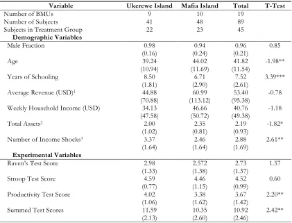
Descriptive statistics about experiment participants are presented in Table 1 and show some of the differences between the samples on each island. Both islands’ participants are predominately male. Ukerewe’s sample is both younger and more educated; however, they also have lower

(11)

ownership, and number of shocks experienced are significantly different between the two islands. Additionally, the residents of Ukerewe Island are predominately Christian while the residents of Mafia Island are predominately Muslim. This is important to note as experiments were run during Ramadan.

Table 1: Descriptive Statistics

---Means with Standard Deviations in Parentheses---

Variable Ukerewe Island Mafia Island Total T-Test

Number of BMUs 9 10 19

Number of Subjects 41 48 89

Subjects in Treatment Group 22 23 45

Demographic Variables

Male Fraction 0.98 0.94 0.96 0.85

(0.16) (0.24) (0.21)

Age 39.24 44.02 41.82 -1.98**

(10.94) (11.69) (11.54)

Years of Schooling 8.50 6.71 7.52 3.39***

(1.81) (2.90) (2.61)

Average Revenue (USD)1 _44.88 _60.99 _53.40 _-0.78

(70.88) (113.12) (95.38)

Weekly Household Income (USD) 34.13 46.66 40.76 -1.18 (47.58) (50.72) (49.38)

Total Assets2 _2.00 _2.35 _2.19 _-1.82*

(1.02) (0.81) (0.93)

Number of Income Shocks3 _3.37 _2.46 _2.88 _2.61**

(1.64) (1.64) (1.69)

Experimental Variables

Raven’s Test Score 2.98 2.572 2.73 1.57

(1.33) (1.38) (1.37)

Stroop Test Score 4.59 4.46 4.52 0.60

(0.77) (1.15) (0.99)

Productivity Test Score 4.02 3.38 3.67 2.20**

(1.06) (1.62) (1.42)

Summed Test Scores 11.59 10.35 10.92 2.42**

(2.13) (2.60) (2.46) *Significant at the 10% level, **Significant at the 5% level, ***Significant at the 1% level

1_{Average revenue from fishing trips in last 30 day}

2 _{Assets: radio, mobile phone, bicycle, television, motor vehicle}

3 _{Income shocks in past 5 years: loss of employment, increase in food prices, decrease in fish prices,}

increase in fishing input prices, household illness, natural disaster, and bad harvest

3.3 Experimental Design

(12)

would handle the problem from a financial side or given options to choose from. For example, one of the questions asked:

“Imagine an unforeseen event requires of you an immediate TSH 130,000 expense. Are there ways in which you may be able to come up with that amount of money on a very short notice? How would you go about it? Would it cause you lasting financial hardship? Would it require you to make sacrifices that have long-term consequences? If so, what kind of sacrifices?”

The treatment group questions were designed to ‘tickle’ the brain so that finances and monetary concerns came to top of mind, simulating financial scarcity, before the rest of the experiment was completed. Participants assigned to the control group were also randomly given one of two questions; however, their questions asked a non-financial hypothetical problem.

Once the question portion of the experiment was complete, both treatment group and control group participants were informed they would be given three sets of tasks to complete. Participants were told they would be paid based on their performance on each task and would receive their payout at the end of the experiment. The first task the participants were asked to complete was the Raven’s Test. Each participant was presented with five trials of six to eight square Raven’s Standard Progressive Matrices. The order of the trials was randomized for each participant to account for any ordering bias that might exist, and participants could take as long as they needed to answer each question. The Raven’s Test is often used to measure IQ and specifically looks at an individual’s ability to think logically and problem solve. The Raven’s Test requires individuals to make meaning out of confusion and replicate information in a way that provides a direct measure of fluid intelligence, or cognitive ability. Most importantly, although the Raven’s Test is often

criticized, the test provides consistent measures of intelligence across different cultures and over time (Raven, 2000; Rushton, Skuy, & Fridjhon, 2003).

(13)

Finally, participants completed the Productivity Test. Adapted from Niederle and

Vesterlund (2005), the Productivity Test gave participants two minutes to solve as many summations of five single digit numbers as possible. Each participant was again given five different trials,

presented in random order. Each problem had to be solved before going on to the next and participants were allowed to use pen and paper to work out the problems. Following the experiment, participants were asked to complete a short survey, which asked them demographic questions, as well as questions about income shocks, physical household characteristics, and children’s health.2

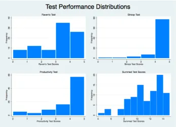
Each participant’s score was tallied upon completing the experiment. Participants received a ‘1’ for correct answers and a ‘0’ for incorrect or unanswered questions. The maximum score a participant could receive was 15. Mean test scores from the experiment are listed at the bottom of Table 1 and show that Ukerewe participants did slightly better than Mafia participants, with the scores for the Productivity Test and the Summed Test scores being significantly different. Figure 1 shows the distribution of scores for each of the three tests, as well as the summed score. Viewing the distributions shows that most scores for the Stroop Test and Productivity Test are on the higher end, while more variation exists for the Raven’s Test scores and the Summed Test scores.

Figure 1: Test Performance Distribution by Test and Frequency

(14)

3.4 Empirical Specification

This study uses OLS regression models to test hypotheses on the impact of the ‘scarcity trigger’ treatment, as well as other measures of scarcity, on cognitive function and productivity. Existing literature suggests that the two main types of scarcities faced by the poor are financial scarcity and mental scarcity; as such the models will test both types of scarcity as well as the interaction between an individual’s existing scarcities and treatment status.

3.4.1 ‘Scarcity Trigger’ Treatment Effect

To estimate the treatment effect of receiving the scarcity treatment on test scores I use the following model:

!"#$%! = !+!!!!!+!!!!+!+!! (1)

The dependent variable, Score, is the score of individual i, on each of the three different tests and the total of the three tests. Separate regressions are run for each test as well as the total. All regressions report individual test scores in standardized format while the total score of all tests for a participant is reported as a summary index (Anderson, 2008). T is the indicator variable for

treatment group assignment. !_!!_!_{represents control variables for each individual including: age,} gender, years of schooling, weekly household income in US Dollars, and question. The question variable controls for any impact the specific treatment or control question might have had on test performance. ! is a BMU level dummy variable that works similarly to a fixed effect and controls for unobservable characteristics between each BMU, as well as differences between Ukerewe Island and Mafia Island. Because standardized and indexed values are used, coefficients are interpreted as an increase or decrease in test score standard deviations. Based on existing literature I expect treatment group status to lower test scores so that the coefficient on T is negative.

3.4.2 The Effect of Existing Mental and Financial Scarcities

In addition to trying to find a casual effect between laboratory simulated scarcity and cognition, I am also interested in whether a correlation exists between the existing financial and mental scarcities in an individual’s life and cognition and productivity. The following OLS model estimates the impact of existing mental and financial scarcities on test performance:

!"#$%_! =!+!_!!"#$_!+!_!!"#$%&&_! +!_!!"#$ℎ!"#$_!+!_!!_!₊_!₊_!

(15)

The dependent variable in this model is exactly the same as in equation (1). Dist is an index of ‘anti-comfort goods’ that serves as a measure of an individual’s level of distraction. Revdiff is the difference in US Dollars between a fisherman’s average revenue from fishing in the last 30 days and the revenue he received on his most recent fishing trip. Numshocks is the total number of income shocks a fisher has experienced in the last five years. !!_!!_!_{and ! represent the same variables from} equation (1). Whether a participant was assigned to the treatment or control group, and any underlying affect treatment arm assignment has on test outcomes is treated as an unobservable characteristic in this model and is therefore assumed to be absorbed by the error term.

The distractions index variable (dist) is based on Banerjee and Mullainathan’s (2008) limited attention and productivity model, which concludes that owning ‘comfort goods’ makes workers less distracted by problems at home when working; therefore, they are more productive and earn higher incomes. Because most fishers in my sample live at subsistence levels, creating an index of comfort goods was not possible. Instead I identified key ‘anti-comfort’ goods and created an index of

‘distractions’ using Anderson’s summary index (2008). Banerjee and Mullainathan list running water, electricity, and a reliable baby sitter as examples of comfort goods. For the purposes of this study, measures of access to clean water sources, electricity, and healthy children are defined as comfort goods. None of the participants in the sample have electricity, therefore, the ‘anti-comfort’ goods used in the distractions index are getting water from an ‘unclean’ source, having a dirt floor, and having children with malaria3_{. Dirt floors act as an additional measure of children’s health per}

Cattaneo, Galiani, Gertler, Martinez, and Titiunik (2009), which finds a correlation between dirt

floors and parasitic infestations in young children. Drinking water from an unclean source is also likely to be correlated with children’s health. The malaria measures report how many children in a household have had malaria in the last year. Although majority of the fishers in my sample are men, and may be less aware of their children’s health issues than women, I believe the men were able to accurately report malaria measures as malaria is a serious illness in Tanzania and is likely to require financial costs. Data used to create the distractions index was taken from responses to the survey each participant took following the experiment.

The unclean water source and dirt floor variables used to create the distractions index are binary indicator variables, taking on a value of ‘1’ if a household gets its water primarily from an unclean source or has a dirt floor, and ‘0’ if otherwise. The malaria variable is a continuous variable

3_{Water from an unprotected well or a lake or river are considered unclean sources according to standards outlined by}

(16)

and responses to the malaria survey question range from zero to six children in a household with malaria. The distractions index variable mean is 0.019 and the standard deviation is 0.609. Because summary index techniques were used the distractions variable is simply the weighted average of unclean water, dirt floors, and malaria measures where weights are constructed from the inverse of the covariance matrix (Anderson, 2008).

The revenue difference variable (revdiff) measures the difference in average fishing revenue earned in the last 30 days compared with the participant’s most recent fishing trip, as is used as a proxy for the relative financial scarcity a fisher may be experiencing at the time the experiment was run. Because Mani, Mullainathan, Shafir, and Zhao’s (2013) run their scarcity experiment on Indian sugarcane farmers before and after harvest, revenue difference tries to replicate this experiment design by looking at whether a fisher’s most recent earnings, relative to his monthly average, impacts test performance. While the revenue difference variable looks at recent scarcities, the number of shocks variable (numshocks) looks at the impact that long run scarcities caused by income shocks in the past five years have on test performance. Fishers were given a total of seven income shocks they could have experienced. The number of shocks variable reports each fisher’s total shocks. Again, based on existing literature I expect the coefficients on all three of the variables in equation (2) to be negative, indicating that an increase in a fishers distractions, revenue difference, or number of shocks decreases his test scores.

3.4.3 ‘Scarcity Trigger’ and Existing Scarcities Interaction

The final model I test considers the impact of the interaction of treatment status and existing mental and financial scarcities:

!"#$%_! = !+!!_!!_!+!_!!"#$_! +!_!!"#$%&&_! +!_!!"#$ℎ!"#$_! +!_!!_!!"#$_! +!_!!_!!"#$%&&_! + !_!!_!!"#$ℎ!"#$_! +!_!!_!₊_!₊_!

! (3)

(17)

experiencing more shocks has an even larger impact on test performance. Again, I expect the coefficients on the interaction variables to be negative.

4. Results

4.1 Empirical Results

4.1.1 Treatment Effect

My first model looks only at treatment status to determine if the treatment group is

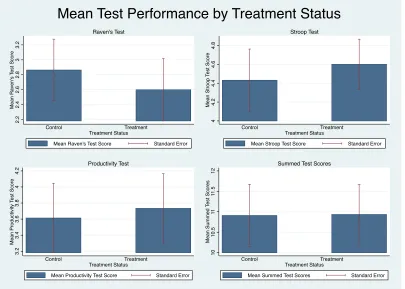
significantly different than the control group. Figure 2 shows the average score for each of the three tests by treatment status plus the average sum of all three tests by treatment. The image shows that the control group had a higher mean score on the Raven’s Test than the treatment group, while the treatment group had a higher mean score on the Stroop Test and Productivity Test. Graphically, the two experimental groups appear to perform about the same when all test score means are summed.

Figure 2: Mean Test Performance by Treatment Status

2.2 2.4 2.6 2.8 3 3.2 Me a n R a ve n 's T e st Sco re Control Treatment Treatment Status

Mean Raven's Test Score Standard Error Raven's Test 4 4.2 4.4 4.6 4.8 Me a n St ro o p T e st Sco re Control Treatment Treatment Status

Mean Stroop Test Score Standard Error Stroop Test 3.2 3.4 3.6 3.8 4 4.2 Me a n Pro d u ct ivi ty T e st Sco re Control Treatment Treatment Status

Mean Productivity Test Score Standard Error Productivity Test 10 10.5 11 11 .5 12 Me a n Su mme d T e st Sco re s Control Treatment Treatment Status

Mean Summed Test Scores Standard Error Summed Test Scores

(18)

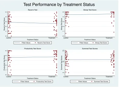
Figure 3 also looks at the test scores by treatment for individual participants and finds evidence that on the Raven’s Test the control group performed a little better. Individuals in the treatment group performed better on the Stroop Test. For the Productivity Test, as well as the summed test scores, participants in the treatment and control groups appear to have performed about the same.

Figure 3: Test Performance by Treatment Status

Running a two-sample t-test on each test score by treatment status finds that the difference in test performance between the two groups is not statistically significant. Table 2 summarizes the t-test results.

Table 2: Test Performance Differences: Treatment vs. Control Status ---Means with t-statistics in

parenthesis---Treatment Group Control Group Difference-in-Means

Raven’s Test 2.60 2.86 -0.264

(0.906)

Stroop Test 4.6 4.43 0.168

(-0.800)

Productivity Test 3.73 3.61 0.120

(-0.396)

Summed Test Score 10.93 10.91 0.024

(-0.046)

Observations 45 44

0 1 2 3 4 5 R a ve n 's T e st Sco re Control Treatment Treatment Status

Fitted Values Raven's Test Score

Raven's Test 0 1 2 3 4 5 St ro o p T e st Sco re Control Treatment Treatment Status

Fitted Values Stroop Test Score

Stroop Test Score

0 1 2 3 4 5 Pro d u ct ivi ty T e st Sco re Control Treatment Treatment Status

Fitted Values Productivity Test Score

Productivity Test Score

5 10 15 Su mme d T e st Sco re s Control Treatment Treatment Status

Fitted Values Summed Test Scores

Summed Test Scores

(19)

Running a regression using the model from equation (1) provides further confirmation: treatment status does not have a significant impact on performance. Regression results are summarized in Table 3. The coefficients on the Raven’s Test treatment variables are negative as predicted, but not significant. In column (1) of panel (A) treatment has a negative coefficient, which indicates that treatment status decreases performance on the Raven’s test by almost 0.20 standard deviations. Once education is controlled for this effect size decrease to just -0.03. Although not significant, the rest of the coefficients are positive, which is not what I expected given existing literature.

Table 3: Treatment Status and Test Scores Dependent Variable: Test Score

--Ordinary Least Squares Estimates, Standard Errors--

Tests & Variables (1) (2)

A. Raven’s Test

Treatment -0.193 -0.029

(0.214) (0.249)

Constant 0.074 -0.393

(0.152) (0.871)

Controls N Y1

Robust Standard Errors N N

R-Squared 0.009 0.074

B. Stroop Test

Treatment 0.162 0.157

(0.202) (0.239)

Constant -0.050 -0.390

(0.144) (0.835)

Controls N Y

R-Squared 0.007 0.026

C. Productivity Test

(0.209) (0.235)

Constant -0.014 -0.600

(0.148) (0.819)

Controls N Y2

R-Squared 0.002 0.117

D. Summary Index Score

(0.132) (0.150)

Constant -0.002 -0.463

(0.094) (0.523)

Controls N Y1

R-Squared 0.001 0.089

Observations 89 86

*** p<0.01, ** p<0.05, * p<0.1

(20)

4.1.2. Mental and Financial Scarcities

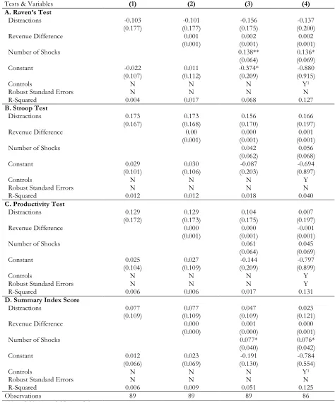
Table 4 shows the results of the OLS regressions that I ran using equation (2). The coefficient on the distractions index is negative for all four Raven’s Test regressions in panel (A), indicating that a one standard deviation increase in distraction levels causes a decrease in Raven’s Test performance. While not statistically significant, the decrease ranges from approximately 0.10 to 0.15 standard deviations. The number of shocks variable has a statistically significant impact on both the Raven’s Test scores and the Summary Index Score when control variables are both

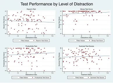
included and excluded, however the coefficients are positive. The revenue difference variable has an effect size of approximately zero, showing that a fisher’s relative wealth when he participated in the study has no effect on his test performance. Figure 4 gives a graphic depiction of the relationship between test performance and distraction levels. The visualization of the data is consistent with the regression results.

Figure 4: Test Performance by Level of Distraction

0 1 2 3 4 5 R a ve n 's T e st Sco re

-1 -.5 0 .5 1 1.5

Distractions Index

Fitted Values Raven's Test Score

Raven's Test 0 1 2 3 4 5 St ro o p T e st Sco re

-1 -.5 0 .5 1 1.5

Distractions Index

Fitted Values Stroop Test Score

Stroop Test Score

0 1 2 3 4 5 Pro d u ct ivi ty T e st Sco re

-1 -.5 0 .5 1 1.5

Distractions Index

Fitted Values Productivity Test Score

Productivity Test 5 10 15 Su mme d T e st Sco re s

-1 -.5 0 .5 1 1.5

Treatment Status

Fitted Values Summed Test Scores

Summed Test Scores

(21)

Table 4: Existing Scarcities and Test Scores Dependent Variable: Test Score

Tests & Variables (1) (2) (3) (4)

Distractions -0.103 -0.101 -0.156 -0.137

(0.177) (0.177) (0.175) (0.200)

Revenue Difference 0.001 0.002 0.002

(0.001) (0.001) (0.001)

Number of Shocks 0.138** 0.136*

(0.064) (0.069)

Constant -0.022 0.011 -0.374* -0.880

(0.107) (0.112) (0.209) (0.915)

Controls N N N Y1

Robust Standard Errors N N N N

R-Squared 0.004 0.017 0.068 0.127

B. Stroop Test

Distractions 0.173 0.173 0.156 0.166

(0.167) (0.168) (0.170) (0.197)

(0.001) (0.001) (0.001)

Number of Shocks 0.042 0.056

(0.062) (0.068)

Constant 0.029 0.030 -0.087 -0.694

(0.101) (0.106) (0.203) (0.897)

Controls N N N Y

R-Squared 0.012 0.012 0.018 0.040

Distractions 0.129 0.129 0.104 0.007

(0.172) (0.173) (0.175) (0.197)

Revenue Difference 0.000 0.000 -0.001

(0.001) (0.001) (0.001)

(0.064) (0.069)

Constant 0.025 0.027 -0.144 -0.797

(0.104) (0.109) (0.209) (0.899)

Controls N N N Y

Robust Standard Errors N N N Y

R-Squared 0.006 0.006 0.017 0.131

Distractions 0.077 0.077 0.047 0.023

(0.109) (0.109) (0.109) (0.121)

(0.000) (0.000) (0.001)

Number of Shocks 0.077* 0.076*

(0.040) (0.042)

Constant 0.012 0.023 -0.191 -0.784

(0.066) (0.069) (0.130) (0.554)

Controls N N N Y1

R-Squared 0.006 0.009 0.051 0.125

Observations 89 89 89 86

*** p<0.01, ** p<0.05, * p<0.1

(22)

4.1.3 The Interaction Effect

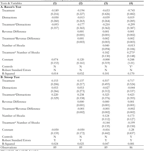
The results of the interaction model presented in equation (3) are summarized in Tables 5 and 6:

Table 5: Interaction of Treatment & Distractions Index and Test Scores: Dependent Variable: Test Score

Tests & Variables (1) (2) (3) (4)

Treatment -0.189 -0.194 -0.653 -0.745

(0.216) (0.227) (0.426) (0.482)

Distractions -0.050 -0.013 -0.039 0.019

(0.260) (0.263) (0.264) (0.285)

Treatment*Distractions -0.093 -0.177 -0.210 -0.299

(0.357) (0.365) (0.362) (0.387)

(0.001) (0.001) (0.002)

Treatment*Revenue Difference 0.001 0.002 0.002

(0.003) (0.003) (0.003)

Number of Shocks 0.040 -0.013

(0.094) (0.106)

Treatment* Number of Shocks 0.182 0.275*

(0.130) (0.148)

Constant 0.074 0.120 -0.000 0.248

(0.153) (0.161) (0.319) (1.01)

Controls N N N Y1

R-Squared 0.014 0.032 0.101 0.170

B. Stroop Test

Treatment 0.153 0.137 0.557 0.717

(0.206) (0.217) (0.493) (0.524)

Distractions 0.053 0.053 -0.027 -0.044

(0.266) (0.273) (0.312) (0.337)

Treatment*Distractions 0.220 0.238 0.323 0.423

(0.329) (0.338) (0.376) (0.393)

(0.001) (0.001) (0.001)

Treatment*Revenue Difference -0.001 -0.001 -0.002

(0.002) (0.002) (0.002)

(0.112) (0.127)

Treatment* Number of Shocks -0.144 -0.199

(0.135) (0.150)

Constant -0.050 -0.050 -0.416 -1.28

(0.159) (0.172) (0.442) (0.837)

Controls N N N Y

Robust Standard Errors Y Y Y Y

R-Squared 0.024 0.025 0.047 0.081

*** p<0.01, ** p<0.05, * p<0.1

(23)

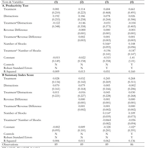
Table 6: Interaction of Treatment & Distractions Index and Test Scores Dependent Variable: Test Score

Tests & Variables (1) (2) (3) (4)

A. Productivity Test

Treatment 0.081 0.114 0.684 0.661

(0.210) (0.223) (0.468) (0.491)

Distractions 0.192 0.186 0.078 0.026

(0.253) (0.258) (0.244) (0.306)

Treatment*Distractions -0.122 -0.146 -0.031 -0.104

(0.348) (0.358) (0.373) (0.403)

Revenue Difference -0.000 0.000 -0.001

(0.001) (0.001) (0.001)

(0.003) (0.003) (0.003)

Number of Shocks 0.166* 0.148

(0.093) (0.096)

(0.141) (0.147)

Constant -0.015 -0.022 -0.515 -1.41

(0.149) (0.158) (0.358) (1.01)

Controls N N N Y

Robust Standard Errors N N Y Y

R-Squared 0.009 0.013 0.051 0.160

B Summary Index Score

Treatment 0.028 0.032 0.245 0.268

(0.134) (0.142) (0.269) (0.311)

Distractions 0.070 0.079 0.005 -0.002

(0.161) (0.164) (0.166) (0.206)

Treatment*Distractions 0.011 -0.016 0.045 0.030

(0.221) (0.227) (0.228) (0.268)

(0.001) (0.001) (0.001)

(0.002) (0.002) (0.002)

Number of Shocks 0.114* 0.109

(0.059) (0.075)

(0.082) (0.094)

Constant -0.002 0.009 -0.328 -1.02*

(0.095) (0.101) (0.201) (0.591)

Controls N N N Y

Robust Standard Errors N N N Y

R-Squared 0.006 0.011 0.062 0.136

*** p<0.01, ** p<0.05, * p<0.1

(24)

significant. Stroop Test regression results in panel (B) of Table 5 yield negative, but insignificant, coefficients on the treatment and distractions interaction variable as well as the treatment and number of shocks interaction variable. Table 6 reports the interaction model results for the

Productivity Test and the Summary Index Score and finds negative coefficients on the interaction of treatment and number of shocks for both, although neither is statistically significant. For all tests, the revenue difference variable and its interaction with treatment status again have approximately zero effect on test performance.

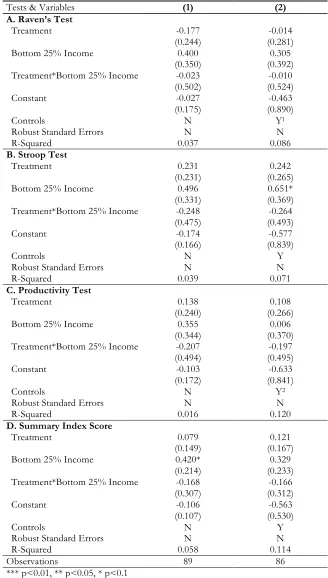
4.1.4 Further Results

Because the interaction of treatment and the existing scarcities in an individual’s life do not yield statistically significant results, I tested one more model as a variation of equation (3) to determine if where a participant’s weekly income falls in the sample’s income distribution impacts test performance. To do this I created indicator variables which would equal ‘1’ if the participant was within a given income quartile and ‘0’ if not. I did this for the measured weekly household incomes that fell in the bottom 25% and top 25% of my sample. I chose 25% because anything smaller did not provide enough variation. These measures allow me to look at whether a participant who is relatively poorer or relatively richer than the rest of the sample performs better or worse on the tests. The interaction with treatment status allows me to determine if the treatment effect was stronger for those who were poorer to begin with.

(25)

Table 7: Test Performance by Weekly Household Income, Bottom 25% Dependent Variable: Test Score

Treatment -0.177 -0.014

(0.244) (0.281)

Bottom 25% Income 0.400 0.305

(0.350) (0.392) Treatment*Bottom 25% Income -0.023 -0.010 (0.502) (0.524)

Constant -0.027 -0.463

(0.175) (0.890)

Controls N Y1

R-Squared 0.037 0.086

B. Stroop Test

(0.231) (0.265)

Bottom 25% Income 0.496 0.651*

Constant -0.174 -0.577

(0.166) (0.839)

Controls N Y

R-Squared 0.039 0.071

(0.240) (0.266)

Bottom 25% Income 0.355 0.006

Constant -0.103 -0.633

(0.172) (0.841)

Controls N Y2

R-Squared 0.016 0.120

(0.149) (0.167)

Bottom 25% Income 0.420* 0.329

Constant -0.106 -0.563

(0.107) (0.530)

Controls N Y

R-Squared 0.058 0.114

Observations 89 86

*** p<0.01, ** p<0.05, * p<0.1

(26)

Table 8: Test Performance by Weekly Household Income, Top 25% Dependent Variable: Test Score

Treatment -0.0954 0.0727

(0.249) (0.276)

Top 25% Income 0.433 1.121**

(0.378) (0.501) Treatment*Top 25% Income -0.464 -0.566 (0.499) (0.515)

Constant -0.015 -0.679

(0.171) (0.865)

Controls N Y1

R-Squared 0.025 0.132

B. Stroop Test

(0.235) (0.270)

Top 25% Income 0.553 0.656

Constant -0.163 -0.567

(0.161) (0.845)

Controls N Y

R-Squared 0.035 0.050

Treatment 0.0585 0.0466

(0.245) (0.214)

Top 25% Income -0.147 0.241

(0.372) (0.520) Treatment*Top 25% Income 0.128 0.0224 (0.491) (0.562)

Constant 0.016 -0.654

(0.168) (0.875)

Controls N Y

Robust Standard Errors N Y

R-Squared 0.004 0.122

(0.155) (0.166)

Top 25% Income 0.279 0.651**

Constant -0.059 -0.630

(0.106) (0.520)

Controls N Y2

R-Squared 0.017 0.141

Observations 89 86

*** p<0.01, ** p<0.05, * p<0.1

(27)

4.2 Empirical Conclusions

The empirical results fail to find that treatment, existing scarcities, or the interaction of the two have a significant impact on test performance. An individual’s relative degree of poverty or wealth compared to the rest of the sample also has no impact. However, the coefficient on the Raven’s Test score is consistently negative and sometimes large for treatment status, the distractions index, and the interaction of the two. This raises the question of whether scarcity does impact cognitive function via the Raven’s Test, but just failed to be found statistically significant in this study. Because the Raven’s test measures the ability to think logically and problem solve absent any prior knowledge, results suggest that scarcity does hinder abstract problem solving, just not

significantly.

5. Discussion

5.1 Experiment Statistical Power

This experiment sought to determine if financial and mental scarcities hinder cognitive function and productivity. Given the study has a sample size of only 89, lack of statistical power may be what is driving the results to be statistically insignificant. Running a power calculation shows that my study has statistical power of 5.1%. This indicates that the study is highly underpowered and rejecting a false null hypothesis is improbable.

(28)

Table 9: Summary of Observed and Estimated Effect Sizes1

Measure Raven’s Test Stroop Test Productivity Test Summed Test Scores

Observed Effect Sizes -0.264 0.168 0.120 0.024

Estimated Minimum Effect Sizes2

-0.826 0.599 0.859 1.484

1 _{Effect sizes calculated as difference-in-means between treatment group and control group} 2 _{Estimated assuming 80% statistical power}

5.2 An Analysis of Three Similar Studies

In order to compare my results to the existing literature that looks at the impact of scarcity on cognitive function and productivity, I calculated the difference-in-means between treatment and control outcomes observed in three similar studies. The first experiment is Mani, Mullainathan, Shafir, and Zhao’s (2013) field study, which surveys Indian sugar cane farmers pre-harvest and post-harvest to measure the impact of scarcity on Raven’s Test accuracy and Stroop Test errors. The difference-in-means observed for the Raven’s Test accuracy and Stroop Test errors are -1.1 and 0.77.

The second study is Shah, Mullainathan, and Shafir (2012), which again looks at the impact of scarcity on cognition, but this time in a laboratory setting. Participants in experiment 1 of this study played games of Wheel of Fortune where participants assigned to the ‘rich’ group received more guesses than participants assigned to the ‘poor’ group. Participants were then asked to complete cognitive control and attention tests. The difference-in-means between ‘poor’ and ‘rich’ participants is -7.81.

The final study I looked at uses happiness levels as a measure of distraction and tests the relationship between happiness and productivity. While the treatment variable differs from my research, the way treatment was administered and overall experiment design used by Oswald, Proto,

and Sgroi (2009) is close to my experiment design. Their model is also based on Banerjee and

Mullainathan (2008), and they use the same productivity test from Niederle and Vesterlund (2005) as

I do. Oswald et al. find a difference-in-means between treatment and control outcomes of 1.71.

Table 10reports the observed difference-in-means for each of these studies.

(29)

Mani, Mullainathan, Shafir, and Zhao (2013) study. Therefore, if my study had more statistical power, I may have been able to find effect sizes consistent with those in existing literature.

Table 10: Summary of Statistical Results of Three Similar Studies

Measure Mani et al. (2013) Raven’s Test

Accuracy

Mani et al. (2013)

Stroop Test Errors Shah et al. (2012) Experiment 1 Oswald et al. (2009) Experiment 1

Difference-in-Means1

-1.1 0.77 -7.81 1.71

T-Statistics2 _-- _-- _-2.03 _1.75

1_{Calculated treatment and control group difference-in-means.}

2_{Test statistics for two means t-tests. Mani et al. excluded from calculations due to unavailability of full information}

needed to complete calculation.

Given the effect sizes observed in existing literature, I tested for the sample size I would need to get similar difference-in-means values. For the Mani, Mullainathan, Shafir, and Zhao (2013) study, I only looked at the Raven’s Test Accuracy in India, as I measured Stroop Test accuracy as opposed to errors in my replication of the experiment. In order to get a comparable effect size my sample size would need to be approximately 30.4_{Currently with 89 participants, my sample is larger}

than what is calculated here. However as previously mentioned, keeping the sample size at 89 but with 80% statistical power, I should be able to find effect sizes similar to those found by Mani et al.

For a similar effect size found by Oswald, Proto, and Sgroi (2009), I would need a sample size of about 470. For the effect size found in Shah, Mullainathan, and Shafir (2012), my sample size would need to be 110. This information about my optimal sample size is inconclusive, as my existing sample size is larger than the lowest of these calculations, while to equal the highest my sample size would need to increase by roughly four.

Although the studies I analyzed find significance in the impact of treatment on cognition and productivity when running OLS regressions, I used immediate form t-tests to determine whether or not the outcome means for treatment versus controls groups are statistically different from one another. A summary of the t-test results is also included in Table 10. Because Mani, Mullainathan, Shafir, and Zhao’s (2013) study did not report the full information needed to run these calculations, I only looked at the experiments conducted by Shah, Mullainathan, and Shafir (2012) and Oswald, Proto, and Sgroi (2009). For Shah et al’s study the null hypothesis can be rejected at the 5% level, indicating task performance outcomes are significantly different between

(30)

the ‘rich’ and ‘poor’ treatment groups. Coming to conclusions about the Oswald et al. t-tests is more difficult. Whether or not a statistically significant difference exists between the treatment and control group in this study depends on whether a one-tailed or a two-tailed hypothesis is being tested. Using a two tailed test fails to reject the null hypothesis. However using a one tailed test, the null is rejected at the 5% level.

5.3 Randomization Inference

This section has gone into detail about the observed statistical power and effect sizes of my experiment and what my effect sizes would be with 80% power. As a further check, I calculate exact p-values based on randomization inference. Randomization inference is a statistical technique where treatment status is repeatedly resampled within a fixed population allowing inferences about causal effects to be made. In practice, a test statistic is first defined and then calculated under all possible permutations of treatment and control assignment. The results produce an exact p-value that represents where the observed test statistic falls in the distribution of all possible test statistics (Friedman, 2012). The p-value is interpreted as the probability of finding an estimated test statistic greater than or equal to the observed test statistic under a sharp null hypothesis of zero causal effect, and is significant when p<0.05. Randomization inference is useful because the method gives the exact sampling distribution for all possible random assignments under the null hypothesis (Gerber & Green, 2012).

Using randomization inference as a thought experiment for how my results might differ with a larger sample size, I resampled my treatment and control groups over 100,000 permutations using difference-in-means as the test statistic. I tested a sharp null hypothesis of zero treatment effect:

!_!:!!_! ! =!!_! !

This indicates that the potential outcome of participants in the treatment group is exactly equal to the potential outcome for participants in the control group. Table 11 reports the result of my

(31)

Table 11: Randomization Inference Results

-- Standard Errors in Parenthesis--

Observed Difference-in

Means Inference P-Value Randomization HHypothesis: 0: Yi(T)=Yi(C)

Raven’s Test -0.264 0.399 Fail to Reject H0

(0.002)

Stroop Test 0.168 0.461 Fail to Reject H0

(0.002)

Productivity Test 0.120 0.712 Fail to Reject H0

(0.001)

Summed Test Score 0.024 0.965 Fail to Reject H0

(0.001)

Observations 89 100,000

*** p<0.01, ** p<0.05, * p<0.1

The randomization inference results support my empirical findings and earlier inference. The treatment effect of my experiment is not statistically significant. This suggests something other than sample size, perhaps experiment design or treatment strength, may be driving my results. However, because the randomization inference results match my experimental results, I have more confidence in my data and empirical findings.

5.4 Experiment Limitations

Knowing that a larger sample size would not change my observed results, the possible limitations of my experiment must be addressed. To start, the treatment I impose on my

participants may be too light. The scarcity trigger treatment is immediate, short lasting, and rests on the following assumptions: the fishers understand the hypothetical scenario of the question and the question causes some psychological or physiological response in the fishers that will impact

subsequent thinking and action. Whether or not the participants understand the question can be determined through their answers, but determining if the treatment did indeed cause a psychological or physiological reaction is difficult.

The short lasting nature of the scarcity treatment is also of concern when considering why negative coefficients were only found for the Raven’s Test. The Raven’s Test was always the first test given following the hypothetical question both fishers in the control and treatment group were asked. For those that were in the treatment group, the effect of the scarcity trigger may have worn off by the time the Stroop and Productivity Tests were given.

(32)

mathematics under a time constraint. Because the individuals in my sample are fishers, one could plausibly assume that they are comfortable working with numbers and doing basic arithmetic, therefore these tests may have been too easy for them compared to the Raven’s Test, which is more abstract and requires a different approach to solving the problems. The distributions of test scores presented in Figure 1 gives strong evidence that this is the case.

Finally, the scarcity treatment may not be affecting test scores because the concept of scarcity is already imbedded in the participants. As fishers living at subsistence levels, the

participants in this study are exposed to uncertainties and scarcities on a daily basis. As such, the scarcity treatment may have no affect on them. Perhaps if my sample had participants from varying wealth levels and several different occupations, my results would have been different. In addition to using a sample with more variation, if I were to re-conduct my experiment, I would need to design a stronger treatment effect, either by making the effect more lasting or finding an effect where the reaction of the participants would be easier to determine. Measuring cortisol levels between fishers in the treatment and control groups could also determine if the treatment questions did indeed induce a physiological response in the participants.

6. Summary and Conclusion

The motivation for this study was to provide a better understanding of the lives of the poor from a behavioral side by determining the impact that the feeling of scarcity has on cognitive function and productivity. Empirical results showed that being exposed to the scarcity treatment does not significantly impact test performance, nor do the existing sources of scarcity and limited attention in the participant’s lives. The results did find that being in the treatment group and having higher distraction levels yield consistently negative coefficients for the Raven’s Test, indicating scarcity may hinder one’s ability to do abstract problem solving, just not significantly. An analysis of the experiment I ran determines that the experiment was underpowered; however, using

randomization inference allows me to have confidence in my empirical findings.

(33)

difficult. Reviewing a wide array of literature in behavioral economics shows that studies that look at the general psychological impacts of poverty are conflicting, inconclusive, and with the exception of a few studies, do not find causal relationships. My study contributes to this literature by adding a new experiment that contradicts existing findings.

Although the experiment was unable to provide solid evidence that scarcities negatively impact cognitive function and productivity, the underlying motivation for researching and

(34)

References

Anderson, M. L. (2008). Multiple inference and gender differences in the effects of early intervention: A reevaluation of the Abecedarian, Perry Preschool, and Early Training Projects. Journal of the American statistical Association, 103(484).

Banerjee, A. V., & Mullainathan, S. (2008). Limited attention and income distribution. American Economic Review, 98(2), 489-493.

doi:http://0dx.doi.org.ignacio.usfca.edu/10.1257/aer.98.2.489

Bertrand, M., Mullainathan, S., & Shafir, E. (2004). A behavioral-economics view of poverty. American Economic Review, 94(2), 419-423.

Butterworth, P., Cherbuin, N., Sachdev, P., & Anstey, K. J. (2012). The association between

financial hardship and amygdala and hippocampal volumes: Results from the PATH through life project. Social Cognitive and Affective Neuroscience, 7(5), 548-556.

Cattaneo, M. D., Galiani, S., Gertler, P. J., Martinez, S., & Titiunik, R. (2009). Housing, health, and

happiness. American Economic Journal: Economic Policy, 75-105.

Chemin, M., De Laat, J., & Haushofer, J. (2013). Negative rainfall shocks increase levels of the stress hormone cortisol among poor farmers in Kenya. (SSRN Scholarly Paper 2294171). Rochester, NY: Social Science Research Network. Retrieved December 18, 2014, from

http://ssrn.com/abstract=2294171.

Duflo, E. (2006). Poor but Rational?. In A. Banerjee, R. Benabou, & D. Mookherjee (Eds.), Understanding Poverty (pp. 367–78). Oxford, England: Oxford University Press.

Evans, G. W., & Schamberg, M. A. (2009). Childhood poverty, chronic stress, and adult working memory. Proceedings of the National Academy of Sciences, 106(16), 6545-6549.

Friedman, Jed. (2012, January 25). Tools of the Trade: estimating correct standard errors in small sample cluster studies, another take.

Retrieved from http://blogs.worldbank.org//impactevaluations/tools-of-the-trade-estimating-correct-standard-errors-in-small-sample-cluster-studies-another-take

Gerber, A. S., & Green, D. P. (2012). Field experiments: Design, analysis, and interpretation. New York,

NY: WW Norton.

Haushofer, J. (2011). Neurobiological poverty traps.

Haushofer, J. (2013). The psychology of poverty: Evidence from 43 countries.

Haushofer, J., & Shapiro, J. (2013). Household response to income changes: Evidence from an unconditional cash transfer program in Kenya.

(35)

Kahneman, D., & Tversky, A. (1979). Prospect theory: An analysis of decision under risk.

Econometrica, 47(2), 263-291.

Lupien, S. J., King, S., Meaney, M. J., & McEwen, B. S. (2001). Can poverty get under your skin? Basal cortisol levels and cognitive function in children from low and high socioeconomic status. Development and Psychopathology, 13(03), 653-676.

Mani, A., Mullainathan, S., Shafir, E., & Zhao, J. (2013). Poverty impedes cognitive function. Science,

341(6149), 976-980.

Mullainathan, S., & Shafir, E. (2013). Scarcity: Why having too little means so much. New York, NY: Times

Books

Mullainathan, S., & Thaler, R. H. (2000). Behavioral economics (NBER Working Paper 7948).

Cambridge, MA: National Bureau of Economic Research. Retrieved April 16, 2014, from http://www.nber.org/papers/w7948.

Niederle, M., & Vesterlund L. (2005) Do women shy away from competition? Do men compete too much?.

(NBER Working Paper 11474). Cambridge, MA: National Bureau of Economic Research. Retrieved April 30, 2014, from http://www.nber.org/papers/w11474.

Oswald, A. J., Proto, E., & Sgroi, D. (2009). Happiness and productivity (IZA Discussion Paper 4645).

Bonn, Germany: IZA Discussion Papers. Retrieved November 6, 2014, from

http://www.iza.org/en/webcontent/publications/papers/viewAbstract?dp_id=4645.

Raven, J. (2000). The Raven's progressive matrices: change and stability over culture and time.

Cognitive psychology, 41(1), 1-48.

Rushton, J. P., Skuy, M., & Fridjhon, P. (2003). Performance on Raven's advanced progressive matrices by African, East Indian, and White engineering students in South Africa. Intelligence, 31(2), 123-137.

Shah, A. K., Mullainathan, S., & Shafir, E. (2012). Some consequences of having too little. Science,

338(6107), 682-685.

Tversky, A., & Kahneman, D. (1974). Judgment under uncertainty: Heuristics and biases. Science,

185(4157), 1124-1131.

World Health Organization. Health through safe drinking water and basic sanitation. Retrieved September

(36)

Appendix I – Experiment Script & Tests

5

Note: Only read italicized instructions aloud.

Materials: Answer Sheet, Task Questions (pre-randomized), timer for productivity test

Set Up: Record Participant number on their Answer Sheet, Get Paper and Pen ready. Enumerator should sit across from the participant, not next to them.

Hello my name is ___________ . Today I am interested in learning about your life and how you fish. In a little bit we are going to ask you to play a game that will help us learn about how your fish. However before playing the game, I am going to ask you a problem-solving question and ask you to complete a series of tasks.

I am now going to ask you a problem-solving question. Please think about the question carefully before answering.

Treatment Question 1

Consider the following problem: Image an unexpected event costs you an immediate TSH 130,000 expense.

Now please answer the following: Are there ways in which you may be able to come up with that amount of money on a very short notice? How would you go about it? Would it cause you long-lasting financial hardship? Would it require you to make sacrifices that have long-term consequences? If so, what kind of sacrifices?

Consider the following problem:

Imagine the nets you use are damaged, but they still work. The cost to repair the nets is TSH 100,000 and you are responsible for paying for the repairs. You need to decide the following:

Read each option first and then ask the participant which one they would choose.

1) Pay the full amount in cash. Would this require you to dip into saving? How you would you go about getting the cash?

2) Take out a loan that would require weekly repayments of TSH 5,000 over 5 months (approx. 10% interest over 20 weeks).

3) Take a chance, don’t repair the nets and hope it lasts a while longer. Of course, this leaves open the possibility of further damage or even greater expenses in the long run.

Which of these options do you choose? Why? Would it require you to make sacrifices that have long-term consequences? If so, what kind of sacrifices?

Consider the following problem:

Suppose there is a bad storm and you must make repairs to your house. To pay for the supplies needed you have two options:

Read each option first and then ask the participant which one they would choose.