#∃∀ % ∀∀ &∀ ∀ !∋ ∀ ()∗+
∋, !∀∀−.. ∀ /.(0.
Keywords: Concurrent Branch Patterns, Concurrent Sequential Patterns (Consp) Mining, Consp-Graph, Graph-Based Modelling, Sequential Patterns Post-Processing, Structural Relation Patterns
1. INTRODUCTION
The goal in patterns mining is to find useful patterns from very large databases. Frequent patterns mining is one of the most important knowledge discovery techniques, which in-cludes frequent itemset mining (Agrawal et al., 1993), sequential patterns mining (Agrawal & Srikant, 1995; Pei et al., 2001; Zaki, 2001), graph mining (Cook & Holder, 2000; Huan et al., 2004) and tree mining (Asai et al., 2002; Zaki, 2005).
While frequent itemset mining aims to find frequent itemsets in a transaction
data-base, sequential patterns mining aims to find
sub-sequences that appear frequently (i.e. more than a given support threshold) in a sequence database. The problem of discovering sequential patterns was first introduced by Agrawal and Srikant (1995) and their approach introduced some of the most important and basic defini-tions in sequential patterns mining. Since then, it has been studied extensively in the literature, resulting in algorithms such as GSP (G eneral-ized Sequential Pattern; Srikant & Agrawal, 1996), FreeSpan (Frequent pattern-projected
Sequential patterns mining; Han et al., 2000), PrefixSpan (Prefix-projected Sequential pa t-terns mining; Pei et al., 2001) and SPADE (S
e-Graph-Based Modelling of
Concurrent Sequential Patterns
Jing Lu, Southampton Solent University, UK
Weiru Chen, Shenyang Institute of Chemical Technology, China
Malcolm Keech, University of Bedfordshire, UK
ABSTRACT
Structural relation patterns have been introduced recently to extend the search for complex patterns often hidden behind large sequences of data. This has motivated a novel approach to sequential patterns post-processing and a corresponding data mining method was proposed for Concurrent Sequential Patterns (ConSP). This article reines the approach in the context of ConSP modelling, where a companion graph-based model is devised as an extension of previous work. Two new modelling methods are presented here together with a construction algorithm, to complete the transformation of concurrent sequential patterns to a ConSP-Graph representation. Customer orders data is used to demonstrate the effectiveness of ConSP mining while synthetic sample data highlights the strength of the modelling technique, illuminating the theories developed.
quential PAttern Discovery using Equivalence classes; Zaki, 2001).
In traditional sequential patterns mining, as the support threshold decreases the number of sequential patterns can increase rapidly, and it is difficult to explore so many patterns or get an overall view of them. As a result, there are some trends to mine a more condensed or constrained set of sequential patterns such as
closed sequential patterns (Yan et al., 2003),
compressed sequential patterns (Chang et al., 2006) and contiguous sequential patterns (Chen & Cook, 2007).
With the successful implementation of efficient and scalable algorithms for mining sequential patterns and their variations, it is natural to extend the scope of previous study to structured data mining – the process of finding and extracting useful information from semi-structured databases – such as graph mining and tree mining.
Graph mining here means either graph-transaction mining or single-graph mining (Ivancsy & Vajk, 2005). In graph-transaction mining the database to be mined is a set of graphs and the purpose of this mining task is to search for sub-graphs which occur at least in a given number of graphs (Inokuchi et al., 2003; Huan et al., 2004). On the other hand, in the single-graph format, the input data of the mining process is a single large graph and reoc-curring sub-graphs are searched in the single graph (Cook & Holder, 2000; Kuramochi & Karypis, 2004).
Tree mining, being another instance of frequent patterns mining, extracts frequent sub-trees from a database of labelled sub-trees (Zaki, 2005). Mining frequent trees is useful in applica-tions like bioinformatics, computer vision, text retrieval, web analysis and so on. For example, Asai et al. (2002) modelled semi-structured data by labelled ordered trees and studied the problem of discovering all frequent tree-like patterns in a given collection of datasets.
In the context of frequent patterns mining, the term pattern refers to itemset, sequence, graph and tree patterns. There are some ques-tions in this area, for example: is it possible to
summarise and represent these patterns? Can any other patterns be discovered beyond these to extend the scope of frequent patterns mining?
For the first question, Zaki et al. (2005) introduced the Data Mining Template Library and provided a description of the graphical representation of these frequent patterns. In particular, with respect to sequential patterns summary and analysis, Lu, Wang et al. (2004) proposed a Sequential Patterns Graph (SPG) as the minimal representation of a collection of sequential patterns. These research areas are discussed further in the Related Work sec-tion below.
For the second question, there is some research on mining more general structured patterns such as partial orders, by summarising sequential data (Garriga, 2005), and structural relation patterns from Post Sequential Patterns Mining (Lu & Adjei et al., 2004).
Garriga (2005) addressed the task of sum-marising sequences by means of local order-ing relationships on items. Their work goes beyond the idea of closed sequential patterns in that they generalised sequential patterns into closed partial orders and modelled the patterns using the concept of a lattice. They showed that post-processing of the closed sequences leads to the generalisation of closed partial orders from sequential patterns.
Post Sequential Patterns Mining (PSPM) is a novel data mining approach that underpins the post-processing of sequential patterns (Lu et al., 2008). The aim of PSPM is to mine structural relation patterns – which include concurrent patterns, exclusive patterns and iterative patterns – motivated by the SPG model of representing the relations among sequential patterns. PSPM can be applied to all of the domains that involve sequential patterns mining and can discover other structured patterns beyond traditional sequences.
PSPM does not mine structures directly from the data, as it takes advantage of PrefixSpan
above: SPG is used to give a summary of all the sequential patterns and the method can be extended to the representation of structural rela-tion patterns, as presented in this article.
Related work is introduced next to provide relevant background on patterns modelling and graphical representation. Following the defini-tion and properties of concurrency in patterns mining, including concurrent sequential and branch patterns, the Concurrent Sequential Pat-terns Graph (ConSP-Graph) model is proposed to represent concurrent sequential patterns graphically. The focus is on the outcome of ConSP mining and two associated modelling methods are presented in the following sec-tion, with worked examples to illustrate the approaches. The penultimate section gives an experimental evaluation using a real and a synthetic dataset, showing the results of ConSP mining and modelling. The article draws to a close by making brief conclusions and indicating a potential application in workflow.
2. RELATED WORK
The aim of this research is the graphical repre-sentation of one of the new structural relation
patterns, namely concurrent sequential pat-terns, to inform the analysis of mining results. This section will first describe two types of related work on patterns modelling to provide further motivation, where the latter is from the authors’ previous research on sequential patterns modelling.
2.1 Graphical Representation of Frequent Patterns
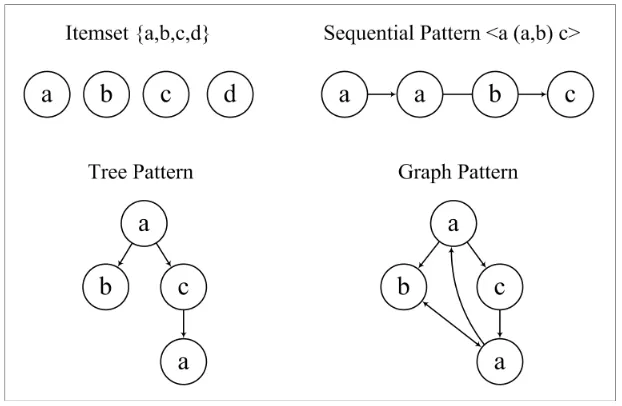
The specific tasks encompassed by frequent pat-terns mining include the mining of increasingly informative patterns in complex structured and unstructured relational data, such as: itemset (transactional, unordered), sequential pattern (temporal or positional), tree pattern (semi-structured, e.g. XML) and graph pattern (com-plex relational). The various frequent patterns mining tasks have different input datasets and generate different forms of results. However, there are inherent relationships among these results such that every pattern can be modelled as a graph, as shown in Figure 1 (Zaki et al., 2005).
Each node is represented by a circle in the figure and node labels are shown inside the circle, with connecting lines (edges) as
appropriate. An itemset is a simple basket of items where no two nodes have the same label. A sequential pattern is modelled as an ordered list of itemsets and thus the different nodes in a sequence can have the same label. Consider the graphical representation of the sequential pattern <a (a,b) c> in the figure; two nodes are labelled as a but they are different because they correspond to two different items a in the sequential pattern <a (a,b) c>. The directed edges indicate the order in a sequence while the undirected edge is used to connect unordered items within the same itemset, e.g. (a,b).
Rooted, ordered and labelled trees are considered more typically in tree mining. A
tree pattern must satisfy all tree properties, namely i) the root has no parent, ii) edges are directed, iii) a node has only one parent, iv) the tree is connected, and v) the tree has no cycles. Finally, it is possible to model any graph pat-tern more generally as shown in the figure; for example connected graphs, induced sub-graphs or directed acyclic graphs.
2.2 Sequential Patterns Graph
In the field of data mining, using graphs is an expressive and versatile modelling technique that provides ways to reason about information implicit in the data. The previous sub-section shows that, as a general data structure, a graph can be used to model complex relations among data and this can be applied specifically to sequential patterns modelling.
In sequential patterns mining, given a customer sequence database and user-specified
minimum support (minsup), a set of sequential patterns (i.e. frequently occurring sub-sequenc-es within the database) can be discovered. All sequential patterns under the specified minimum support can be generated from the Maximal Sequence Set (MSS). Thus, a directed acyclic graph called Sequential Patterns Graph (SPG) was defined to represent the maximal sequence set (Lu, Wang et al., 2004). Nodes (i.e. items or itemsets) of SPG corresponded to elements in a sequential pattern and directed edges were used to denote the sequence relation between two elements. Figure 2 shows two equivalent SPGs that model the same set of maximal sequences,
MSS={xab, xad, yad}.
SPG can be viewed as the visual embodi-ment of the relationship among sequential patterns. Two special types of nodes called a start node (represented by double circles) and a final node (represented by a bold circle) were defined to indicate the beginning and end of maximal sequences. Any path from a start node to a final node corresponds to one maximal sequence. SPG is also the minimal representa-tion of a collecrepresenta-tion of discrete sequential pat-terns; for example Figure 2 represents all the sequential patterns xa, xb, xd, ab, ad, ya, yd,
xab, xad, yad.
SPG is used to give a summary of all the sequential patterns as well as describing the inherent relationship among sequences – the method can be extended for the representation of structural relation patterns (e.g. concurrent se-quential patterns) as presented in this article.
3. COnCURREnCY AnD
PATTERNS REPRESENTATION
Structural relation patterns have been defined in Lu et al. (2008), where a corresponding data mining method and algorithms have been presented. It was also indicated in the previous work that concurrent patterns could be refined further to provide more meaningful information. This section will focus on concurrent sequential patterns and their graphical representation.
3.1 Concurrent Patterns
The fundamental concepts related to sequential patterns are covered extensively in the literature (Agrawal & Srikant, 1995; Pei et al., 2001; Zaki, 2001). For the following definitions, it is assumed that {sp1,sp2,…,spm}is the set of
m sequential patterns mined under minimum support minsup and they are not contained in each other.
Deinition 1. The concurrence of sequential patterns sp1,sp2,…,spk (1≤k≤m) is deined
as the fraction of data sequences that con-tains all of the sequential patterns. This is denoted by
concurrence(sp1,sp2,…,spk)=|{C:∀i (i=1,2,… ,k) spi∠C, C∈SDB}|/|SDB|
where SDB is a sequence database, spi∠C
represents sequential pattern spi contained in data sequence C and the symbol |…| denotes the number of data sequences.
Deinition 2. Let mincon be the user-speciied
minimum concurrence. If
concurrence(sp1,sp2,…,spk)≥mincon
is satisfied, then sp1,sp2,…,spk are called Con-current Sequential Patterns. This is represented by ConSPk=[sp1+sp2+…+spk], where k is the number of sequential patterns which occur
together and the notation ‘+’ represents the concurrent relationship.
Example 1. Consider a sequence database SDB={<a (a,b,c) (a,c) d (c,f)>, <(a,d) c (b,c) (a,c)>, <(e,f) (a,b) (d,f) c b>, <e g (a,f) c b c>} and assume a mincon of 50%. Since both data sequences <(e,f) (a,b) (d,f) c b> and <e g (a,f) c b c> support sequential patterns ebc, eacb, efcb
and fbc under a minsup of 50%, then:
concurrence(ebc, eacb, efcb, fbc)=2/4=50%.
Therefore, they constitute a con-current sequential pattern given by
ConSP4=[ebc+eacb+efcb+fbc].
Using the above definitions, the problem of concurrent sequential patterns mining can be stated as follows: given a sequence database
SDB and sequential patterns mining results (i.e. sequential patterns which satisfy a minimum support threshold), concurrent sequential patterns mining aims to discover the set of all concurrent sequential patterns within a given user-specified minimum concurrence.
Given sequential patterns x, y and z, two features of concurrent sequential patterns and the ‘+’ operator are stated in the following rules:
• Commutative rule: [x+y]=[y+x]
• Associative rule:
[x+y+z]=[[x+y]+z]=[x+[y+z]].
Taking a further look at the concurrent sequential pattern ConSP4 from Example 1, it is clear that some sequential patterns have a
common prefix and/or common postfix, e.g.
eacb and efcb share e and cb. Factoring out
the common prefix and/or postfix can lead to
another type of pattern called a Concurrent Branch Pattern or CBP. The theorem below builds on concurrent sequential patterns and introduces CBP more formally.
ConSPn=[x 1y+x 2y+…+x ny]
where (x iy∈SP, 1≤i≤n; i∈SP; x,y∈SP or
x,y=∅), then the following new pattern can
be deduced:
x[ 1+ 2+…+ n]y.
The above pattern is called a Concur-rent Branch Pattern (CBP) and the notation [ 1+ 2+…+ n] represents n branches of a CBP.
Proof: For simplicity, let us first con-sider n=2. i.e. ConSP2=[x y+x y] (where
x,y, , ∈SP). Sequential patterns x y and x y make up one concurrent sequential pattern that satisfies the concurrence condition (i.e.
concurrence(x y,x y)≥mincon). Therefore, for any data sequence C which supports patterns
x y and x y, there is at least one and one occurring in C. There is at least one x before and one y after ; one x before and one y
after . Thus it can be concluded that there is at least one x before and and at least one y
after and . Hence, the sequence C supports
x[ + ]y and the theorem is proven for n=2. That is, any sequence which supports the concurrent sequential pattern [x y+x y] must support the concurrent branch pattern x[ + ]y.
Secondly, let us consider the case when
n=3, i.e. ConSP3=[x y+x y+x y] (where
x,y, , , ∈SP). Sequential patterns x y, x y and x y make up one concurrent sequential pattern that satisfies the concurrence condi-tion (i.e. concurrence(x y,x y,x y)≥mincon). According to the associative law of concurrent sequential patterns when n=2, x[ + ]y and x y are concurrent. Therefore, from the above case for n=2, x[ + + ]y is also a concurrent branch pattern.
The rest may be deduced by analogy and induction. Hence, the theorem is proven.
As a corollary to the above, we state an-other rule:
Distributive rule: [x +x ]=x[ + ]; [ y+ y]=[ + ]y; [x y+x y]=x[ + ]y.
E x a m p l e 2. F o r C o n S P4 = [ebc+eacb+efcb+fbc] in Example 1, one can take out the common prefix e and postfix cb
from sequential patterns eacb and efcb to yield a concurrent branch pattern e[a+f]cb; similarly, [e+f]bc can be generated by taking out the com-mon postfix bc from ebc and fbc.
Note that in a CBP such as e[a+f]cb, the order of branches a and f is indefinite. Therefore
e[a+f]cb can appear in a sequence database in the form of eafcb or efacb for example. Also, note that neither eafcb or efacb can be discovered from traditional sequential patterns mining with a minsup of 50%.
3.2 ConSP-Graph
The use of graphical models in data mining has led to the development of a sequential patterns model that explores the inherent relationship among sequential patterns. The idea is adapted here for modelling concurrent sequential pat-terns. The definition of SPG (Lu & Wang et al., 2004) is extended to define Concurrent Sequential Patterns Graph and followed by an example for illustration.
Deinition 3.Concurrent Sequential Patterns Graph (ConSP-Graph) is a graphical representation of concurrent sequential patterns denoted by a 7-tuple expressed as: ConSP-Graph=(V, E, S, F, S’, F’, ), where
1. V is a nonempty set of nodes. Each item
(or itemset) in ConSP corresponds to one node in ConSP-Graph and each node in ConSP-Graph at least cor-responds to one item in ConSP. 2. E is a set of directed edges. The
3. S is a set of start nodes, S⊆V, and S≠∅.
There are no start nodes that have the same value in ConSP-Graph.
4. Fis a set of final nodes, F⊆V, and F≠∅.
There are no final nodes that have the same value in ConSP-Graph.
5. S’ is a set of synchronizer nodes, S’⊆V,
with two or more incoming sequential relations applied to concurrent paths to allow no more than one outgoing sequential relation.
6. F’ is a set of fork nodes, F’⊆V,
allowing independent execution between concurrent paths, modelled by connecting two or more outgoing sequential relations.
7. is a function from a set of directed edges to a set of pairs of nodes. can also be defined as a map function of
V V, which indicates the relations between any two nodes.
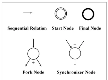
For any node in ConSP-Graph, the subse-quent paths of it cannot be the same, and the ancestor paths of it cannot be the same either. For each pair of different nodes in ConSP-Graph, if they have the same value, there must be different ancestor paths and subsequent paths for them. Graphical elements used in relation to ConSP-Graph are shown in Figure 3, where ‘+’ represents the concurrent relationship across connected paths.
Example 3. The concurrent sequential pattern ConSP4=[ebc+eacb+efcb+fbc] from Example 1 can be cast into its equivalent graphi-cal representation in Figure 4.
Nodes e and f inside the double circles are the start nodes, while nodes b and c inside bold
Figure 3. ConSP-Graph elements
circles are the final nodes. Node e is also a fork node connecting three outgoing sequential rela-tions acb, fcb and bc. Node c is a synchronizer node with two incoming sequential relations
ea and ef; similarly for node b. The refine-ment of concurrent sequential patterns and construction of ConSP-Graph are discussed in the next section.
4. CONCURRENT SEQUENTIAL
PATTERnS MODELLinG
The natural way to approach transforming concurrent sequential patterns to a graphical representation, ConSP-Graph, is by identifying the inherent relationships through common
pre-fix/postfix recognition. This section discusses
two methods to model concurrent sequential patterns: one is refining and combining graphs successively, while the other is based on con-structing graphs step-by-step.
4.1 From Concurrent Sequential Patterns to ConSP-Graph
Given a concurrent sequential pattern
ConSPn={ i| i∈SP, 1≤i≤n, n is the number of sequential patterns in ConSPn}, it tells you that all these sequential patterns will occur together within a concurrence threshold. However, this is not the minimal representation of these sequential patterns because any further relation-ships among them have not been explored. For example, some of them may share the same
prefix and/or postfix and, in that case, we would
want to use a model to predict what will happen concurrently after the prefix item(s) or what will cause the possibility of a postfix item(s).
There are five steps in the following method of modelling a concurrent sequential pattern ConSPn.
1. Initialisation: Represent each sequential pattern in ConSPn by a directed graph G( i) and specify the initial overall model as the union of these graphs – i.e. G=G( 1) ∪ G( 2)
∪ …∪G( n) – initialise a transitional graph model G’=∅.
2. Refinement: For all pairs of G( i) and G( j) in G, where i≠j, refine the overall model by finding each occurrence of a common
prefix and/or postfix – if a pair of graphs share a common prefix/postfix, then go to
Step 3 – otherwise continue through each remaining pair of graphs in G until this cycle is complete, then go to Step 4. 3. Combination: Combine two graphs G( i)
and G( j) which share a common prefix and/ or postfix and generate a new graph – ac-cumulate this new graph in the transitional model G’ – go back to Step 2.
4. Deletion: Delete all graphs from G which have been used successfully for combining as new graphs and include all the combined graphs from G’ to form a new overall model G.
5. Iteration: Repeat Steps 2 to 4 until there are no further successful combinations of pairs of graphs – the final result G is the Concurrent Sequential Patterns Graph,
ConSP-Graph.
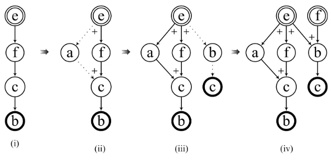
Example 4. For the concurrent sequential pattern ConSP4=[ebc+eacb+efcb+fbc] from Example 1, Figure 5 is a graphical illustra-tion of the procedure of modelling ConSP and highlights the above method.
Further explanation of steps (i) to (v) in Figure 5 is covered below:
1. Initialisation: Represent each sequential pattern in ConSP4 by directed graphs G(1), G(2), G(3) and G(4), the overall initial model G being the union of these graphs, i.e. as shown in Figure 5(i).
2. Refinement: For all pairs of directed graphs in G, refine the overall model by finding each occurrence of a common prefix
and/or postfix, e.g. G(1) and G(2) share a
3. Combination: Combine G(1) and G(2) which share prefix e into G(12), and simi-larly generate new graphs G(13), G(14) and G(23), as shown in Figure 5(ii) – accumu-late these new graphs in the transitional model G’.
4. Deletion: Delete all the graphs from G in Figure 5(i), as they have been used already in Step 3, and include all the combined graphs from G’ to form the new overall model G in Figure 5(ii).
5. Iteration: Repeat Steps 2 to 4. G(12) and G(13) share a common prefix e, so that G(123) can be generated, and G(12) and G(13) can be deleted – see Figure 5(iii). Subsequently, G(23) can be deleted because it is contained by G(123), which leads to Figure 5(iv).
The final combination is then processed for this example and the result is shown in Figure 5(v) – it represents a graphical form of the concurrent sequential pattern
ConSP4=[ebc+eacb+efcb+fbc].
4.2 An Alternative Approach Using SPG
The definition of ConSP-Graph is an exten-sion of that for Sequential Patterns Graph and therefore the method to construct SPG could also be used for ConSP modelling, as described below.
1. Initialisation: Determine the longest length m of sequential patterns in ConSPn
– represent one of the longest sequential patterns by a directed graph G – sort the remaining patterns in order of length.
2. Construction: For the next available sequential pattern sp in ConSPn, find any
common prefix and/or postfix with G – if they share a common prefix/postfix, then
use the Algorithm below to construct the next transitional graph model G – otherwise represent sp by a separate graph G’ and set G=G∪G’.
3. Iteration: For the remaining sequential patterns in ConSPn, which have the same or shorter length – i.e. m, m-1, m-2, etc. – repeat Step 2 incrementally until there are no sequential patterns left in ConSPn. The final result G is the ConSP-Graph.
The algorithm below shows the pseudo-code for the ConSP-Graph construction phase above by adapting the approach for SPG model-ling (Lu, 2006).
ConSP-Graph Construction Algorithm
Input: A sequential pattern sp from concurrent sequential pattern ConSPn
and a transitional graph model G Output: New directed graph G after in-cremental construction
Procedure:
preS=common prefix of sp and G
postS=common postfix of sp and G
elemS=sp-preS-postS
Represent elemS by the directed graph G’IfpreS is not empty
{The last node of preS in G is a fork node;
Add a directed edge from it to the first node of G’;
Mark the connected paths with a ‘+’} IfpostS is not empty
{The first node of postS in G is a synchronizer node;
Add a directed edge to it from the last node of G’;
Mark the connected paths with a ‘+’}
This new directed graph includes a new pattern
sp and is called G.
Example 5. Using the extension of the SPG method to model the concurrent sequential pat-tern ConSP4=[ebc+eacb+efcb+fbc].
1. Initialisation: Determine the longest se-quential patterns in ConSP4, i.e. efcb and
eacb. Represent one of them by a directed graph G – e.g. efcb – see Figure 6(i). 2. Construction: For the next available
se-quential pattern, eacb in ConSP4, find any common prefix preS with G – this is e; and find any common postfix postS – this is cb. Taking out preS and postS from eacb, the remaining part elemS=a can be represented by a directed graph G’. Add a directed edge from the last node of preS in G (i.e.
e) to the first node of G’ (i.e. a) – e is a fork node – mark the connected paths with ‘+’. Also add a directed edge from the last node of G’ (i.e. a) to the first node of postS
(i.e. c) – c is a synchronizer node – mark the connected paths with ‘+’. The result of this step is the graph shown in Figure 6(ii), where the dotted line represents the new edges in the transitional model. 3. Iteration: For the remaining sequential
patterns in turn, i.e. ebc and fbc, construct new graphs in a similar manner. Figure 6(iii) shows the graph after adding sequential pattern ebc and Figure 6(iv) is the final result of this method, which is the same as the graph Figure 5(v).
The above example shows that extending the method of SPG modelling to ConSP-Graph construction is more straightforward in prin-ciple. It corresponds to incremental progression of the transitional graph model as opposed to the pairwise refinement and combination of directed graphs in the method of the previous sub-section.
5. EXPERiMEnTAL
EVALUATION
a synthetic sample. The method and algorithms are implemented using Microsoft Visual C++ where, to mine the sequential patterns, we use the PrefixSpan algorithm. It is available from the IlliMine system package, a partially
open-source data mining package: http://illimine. cs.uiuc.edu/, last accessed 12 May 2009.
5.1 Customers Orders Dataset
A real dataset pertaining to customer purchase data is obtainable from Blue Martini’s Customer
Interaction System in the public domain, http://
cobweb.ecn.purdue.edu/KDDCUP/, last ac
-cessed: 12 May 2009. Three categories of data, i.e. Customer information, Orders information and Click-stream information are collected by the Blue Martini application server and further details about the data are provided in Kohavi et al. (2000).
The Orders dataset corresponds to cus-tomer purchase data made up of customer IDs,
order IDs and product IDs. It contains data collected from 1,821 customers’ behaviour between 28 January 2000 and 31 March 2000, and it includes 3,420 records (i.e. 3,420 pur-chases), 1,917 orders and 999 different kinds of product. Table 1 illustrates the format and contents of the Orders data.
Sequential Patterns Mining
Table 2 illustrates the relationship between
minsup and the number of sequential patterns found in the Orders dataset, where sequential patterns mining has been performed using PrefixSpan (Pei et al., 2001).
The table shows that, when minsup=0.2%, there are 201 sequential patterns with a unique item and there are 17 sequential patterns with two items. Note that a sequence of length k is known as a k-sequence; some of the 2-sequences among the 17 in Table 2 are (41929 41941), (38517 38533), (38537 38533) and (40141 40145). For example, (38517 38533) shows that 0.2% of customers who purchased product 38517 also bought product 38533.
Concurrent Sequential Patterns Mining
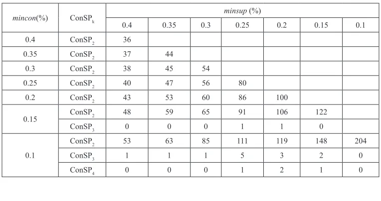
Using the method and algorithms described in Lu et al. (2008), Table 3 shows the extent of the concurrent sequential patterns mining results under various minsup and mincon.
It is shown from Table 3 that, for example when minsup=0.2% and mincon=0.1%, one hundred and nineteen ConSP2, three ConSP3 and two ConSP4 are mined. The specific results for ConSP3 and ConSP4 here are:
Table 1. Format/content of the orders dataset
Customer ID Order ID Product ID … … … 62 3550 19155
62 30018 40393
96 100 13147
132 136 13147
168 832 14135
184 4124 40353
184 4124 44477
184 4124 45371
184 23126 35289
224 228 13143
224 228 14087
236 3412 44449
236 30078 37901
… … … 236 30078 51231
236 30090 39913
236 30090 39917
236 30090 37985
236 30090 38309
236 30090 39727
36 30090 40313
236 30090 40353
… … …
Table 2. minsup and k-sequences on the orders dataset
minsup (%) Number of k-sequences
1-sequence 2-sequence 3-sequence 0.4 74 1
-0.35 90 4
-0.3 112 11
-0.25 163 11
-0.2 201 17
-0.15 261 39 1
[48005+39961+39969] [38545+35273+45363] [40013+39945+39953] [40013+39945+40005+39941]
[45375+(35277,35265)+(35277,35273)+(352 65,35273)]
For instance consider the first ConSP3, [48005+39961+39969]; it shows that at least 0.2% of customers purchased products 48005, 39961 and 39969 concurrently (within a 0.1% concurrence degree). Comparing this ConSP3 with the sequential patterns mining result in Table 2, for example when minsup=0.2%, there are no sequential patterns with length more than 2, i.e. no 3-sequence or 4-sequence either. Therefore, the concurrent sequential patterns ConSP3 and ConSP4 are new structured pat-terns which cannot be discovered by traditional sequential patterns mining.
The equivalent ConSP-Graphs for this real dataset show no connectivity or structure how-ever, so we next use a more illustrative example to take the mining of concurrent sequential patterns to the modelling stage.
5.2 Synthetic Sample
This sub-section presents a complete synthetic example to highlight the concurrent sequential patterns mining and modelling method overall. The sequence database from Example 1 has been chosen as the sample dataset: SDB={<a (a,b,c) (a,c) d (c,f)>, <(a,d) c (b,c) (a,c)>, <(e,f) (a,b) (d,f) c b>, <e g (a,f) c b c>}.
Sequential Patterns Mining
The SDB here has also been used as an example to explain sequential patterns mining when using the Prefixspan algorithm (Pei et al., 2001). The output from this algorithm is listed in Table 4 when the user-specified minimum support (minsup) is set to 50%, where line number identifiers are shown for each of the 67 sequential patterns mined.
Concurrent Sequential Patterns Mining
Concurrent sequential patterns can be mined using the method in Lu et al. (2008) and, when mincon is set to 50%, the results com-prise: [6+41+44], [11+36+62], [16+43+49], [23+63+65] and [52+56+66+67].
Table 3. Concurrent sequential patterns mining on the orders dataset
mincon(%) ConSPk minsup (%)
0.4 0.35 0.3 0.25 0.2 0.15 0.1
0.4 ConSP2 36
0.35 ConSP2 37 44
0.3 ConSP2 38 45 54
0.25 ConSP2 40 47 56 80
0.2 ConSP2 43 53 60 86 100
0.15 ConSP2 48 59 65 91 106 122 ConSP3 0 0 0 1 1 0
0.1
ConSP2 53 63 85 111 119 148 204
ConSP3 1 1 1 5 3 2 0
It can be seen that there are five concurrent sequential patterns and, by replacing the identi-fiers within the patterns by the corresponding sequential patterns in Table 4, the ConSP results at this stage are:
[f+abc+acc] [ab+(a,b)f+(a,b)dc] [bc+acb+dcb] [dc+a(b,c)(a,c)+accc] [ebc+fbc+eacb+efcb]
ConSP Modelling
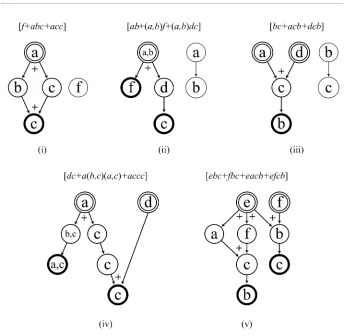
ConSP-Graphs can be generated from these concurrent sequential patterns by using either of the modelling methods in this article. Figure 7 gives the final ConSP modelling results.
ConSP modelling presents a useful vi-sualisation here from which (e.g.) several concurrent branch patterns can be deduced. In Figure 7(i), associated with nodes b and c, the
fork node a and synchronizer node c make up a cycle graph – a graph that consists of a single cycle – therefore a single concurrent branch pattern a[b+c]c can be identified alongside the freestanding node f .
The fork node (a,b) in Figure 7(ii) deter-mines a new concurrent branch pattern (a,b) [f+dc]; similarly, [a+d]cb is another CBP linked through the synchronizer node c in Figure 7(iii). There is also one fork node a and one synchro-nizer node c in Figure 7(iv) and, as they are not part of a cycle graph, two CBPs pertain in this case, i.e. a[(b,c)(a,c)+ccc] and [acc+d]c.
Finally, consider the ConSP-Graph in Figure 7(v), which represents greater complex-ity than the other four. The concurrent branch pattern e[a+f]cb can be generated as an exten-sion of a cycle graph, which contains the fork node e and synchronizer node c; the pattern [e+f]bc is due to the synchronizer node b; and fork node e contributes to another two CBPs, namely e[acb+bc] and e[fcb+bc].
Table 4. Sequential patterns mining results (minsup=50%)
1 (a) 18 (b) (f) 35 (a b) (d) 52 (e) (b) (c)
2 (b) 19 (c) (a) 36 (a b) (f) 53 (e) (c) (b)
3 (c) 20 (c) (b) 37 (b c) (a) 54 (e) (f) (b)
4 (d) 21 (c) (c) 38 (b c) (c) 55 (e) (f) (c)
5 (e) 22 (d) (b) 39 (b c) (a c) 56 (f) (b) (c)
6 (f) 23 (d) (c) 40 (a) (b) (a) 57 (f) (c) (b)
7 (a b) 24 (e) (a) 41 (a) (b) (c) 58 (a) (b) (a c)
8 (a c) 25 (e) (b) 42 (a) (c) (a) 59 (a) (c) (a c)
9 (b c) 26 (e) (c) 43 (a) (c) (b) 60 (a) (b c) (a)
10 (a) (a) 27 (e) (f) 44 (a) (c) (c) 61 (a) (b c) (c)
11 (a) (b) 28 (f) (b) 45 (a) (d) (c) 62 (a b) (d) (c)
12 (a) (c) 29 (f) (c) 46 (b) (d) (c) 63 (a) (b c) (a c)
13 (a) (d) 30 (a) (a c) 47 (c) (b) (c) 64 (a) (c) (b) (c)
14 (a) (f) 31 (a) (b c) 48 (c) (c) (c) 65 (a) (c) (c) (c)
15 (b) (a) 32 (b) (a c) 49 (d) (c) (b) 66 (e) (a) (c) (b)
16 (b) (c) 33 (c) (a c) 50 (e) (a) (b) 67 (e) (f) (c) (b)
It can be seen that the models in Figure 7 bring together connectivity and structure, which opens up further pattern discovery through concurrent branch patterns. More generally, ConSP modelling can add value to the results of concurrent sequential patterns mining by providing a visualisation of otherwise intangible (algebraic) patterns.
In summary, the real dataset used in the previous sub-section aims to show the experi-mental results of mining from the application perspective, while the synthetic example here serves to demonstrate the strength of the graph-based modelling developed in the article. The ConSP mining approach can indeed mine new patterns effectively, beyond sequential orders,
and this new knowledge can be modelled in a meaningful way to represent the inherent structural relationships.
6. CONCLUSION
The refinement of concurrent sequential pat-terns and generation of graph-based models are the main challenges pursued in this article. It is shown that the expression and construction method of sequential patterns graph can be ex-tended to concurrent sequential patterns model-ling, where the features of ConSP-Graph make it straightforward to model the common prefix or postfix elements of concurrent sequential
patterns. A construction algorithm is proposed which is based on SPG and instrumental in the transformation of concurrent sequential patterns to a ConSP-Graph representation.
A real dataset Orders from Blue Martini’s website and synthetic sample data have been used in the experiments to present the results from ConSP mining and modelling, while con-trasting with sequential patterns mining. This has shown that patterns otherwise hidden behind the data can be discovered through concurrent sequential patterns mining and represented by a graphical model. The synthetic sample in particular shows that new concurrent branch patterns can be deduced from graph-based modelling, adding value to the mining results and pointing a further way forward.
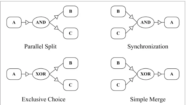
There are potentially related applications for ConSP mining and modelling, for example in the area of workflow induction, a tech-nique to solve a problem in workflow model design (Herbst, 2000). Basic control patterns of workflow can be defined (van der Aalst et al., 2003) which, besides sequence, comprise
parallel split, synchronization, exclusive choice
and simple merge. Figure 8 shows these four constructs graphically.
The parallel split pattern allows a single thread of execution to be split into two (or more) branches which can execute tasks con-currently – it is equivalent to the fork node in ConSP-Graph. Synchronization comes into play once the control node receives input on one of its incoming branches, at a point in the workflow process where multiple parallel activities converge into one single thread of execution – it is equivalent to the synchronizer node in ConSP-Graph.
Taking workflow logs as source data, and following sequential patterns mining, one can apply ConSP mining and modelling to represent fundamental activities and events in order to provide a practical workflow scheme. And, with reference to structural relation patterns more generally (Lu et al., 2008), the concept of exclusive patterns would naturally extend to the
exclusive choice and simple merge constructs in Figure 8 – the subject of future work.
REFERENCES
Aalst, W. M. P., van der Hofstede, A. H. M., ter Kiepuszewski, B., & Barros, A. P. (2003). Workflow patterns. Distributed and Parallel Databases, 14(3), 5–51. doi:10.1023/A:1022883727209
Agrawal, R., Imielinski, T., & Swami, A. (1993). Mining association rules between sets of items in large databases. Proceedings of the 1993 ACM (SIGMOD) (pp.207-216).
Agrawal, R., & Srikant, R. (1995). Mining sequen-tial patterns. In Proceedings of 11th International Conference on Data Engineering (pp. 3-14). Taipei, Taiwan: IEEE Computer Society Press.
Asai, T., Abe, K., Kawasoe, S., Arimura, H., Sata-moto, H., & Arikawa, S. (2002). Efficient substructure discovery from large semi-structured data. In Pro-ceedings of the 2nd SIAM International Conference on Data Mining (Vol. [). Arlington, VA, USA.]. E (Norwalk, Conn.), 87-D(12), 2754–2763.
Chang, L., Yang, D. Q., Tang, S. W., & Wang, T. (2006). Mining compressed sequential patterns. In
Proceedings of the 2nd International Conference on Advanced Data Mining and Applications (Vol.4093, pp.761-768). Xian, China.
Chen, J., & Cook, T. (2007). Mining contiguous sequential patterns from web logs. In Proceedings of the 16th international conference on World Wide Web (pp.1177-1178). Banff, Alberta, Canada. Cook, D. J., & Holder, L. B. (2000). Graph-based data mining. IEEE Intelligent Systems, 15(2), 32–41. doi:10.1109/5254.850825
Garriga, G. C. (2005). Summarizing sequential data with closed partial orders. In Proceedings of the SIAM International Conference on Data Mining
(pp.380–391). California, USA.
Han, J. W., Pei, J., Mortazavi-Asl, B., Chen, Q., Dayal, U., & Hsu, M. C. (2000). Freespan: frequent pattern-projected sequential patterns mining. In Proceedings of the 6th ACM SIGKDD International Conference on Knowledge Discovery and Data Mining (pp.355-359). New York: ACM Press.
Herbst, J. (2000). Dealing with concurrency in work-flow induction. In Proceedings of the 7th European Concurrent Engineering Conference, Society for Computer Simulation (pp.169-174).
Huan, J., Wang, W., Prins, J., & Yang, J. (2004). SPIN: Mining maximal frequent subgraphs from graph databases. Proceedings of the 10th ACM (SIGKDD) (pp. 581-586). Seattle, USA.
Inokuchi, A., Washio, T., & Motoda, H. (2003). Complete mining of frequent patterns from graphs: mining graph data. Machine Learning, 50(3), 321–354. doi:10.1023/A:1021726221443
Ivancsy, R., & Vajk, I. (2005). A survey of discov-ering frequent patterns in graph. In Proceedings of Databases and Applications (pp. 60-72). Calgary, Canada: ACTA Press.
Kohavi, R., Brodley, C., Frasca, B., Mason, L., & Zheng, Z. J. (2000). KDD-Cup 2000 Organizers’ Report: Peeling the onion. SIGKDD Explorations,
2(2), 86–98. doi:10.1145/380995.381033
Kuramochi, M., & Karypis, G. (2004). GREW-A scalable frequent subgraph discovery algorithm. In
Proceedings of the 2004 IEEE International Confer-ence on Mining (pp. 439-442). Brighton, UK. Lu, J. (2006). From Sequential Patterns to Concur-rent Branch Patterns: A new post sequential patterns mining approach. Unpublished doctoral dissertation, University of Bedfordshire, UK.
Lu, J., Adjei, O., Chen, W. R., & Liu, J. (2004). Post Sequential Patterns Mining: A new method for discovering structural patterns. In Proceedings of the Second International Conference on Intelligent Information Processing (pp.239-250). Beijing, China: Springer-Verlag.
Lu, J., Chen, W. R., Adjei, O., & Keech, M. (2008). Sequential patterns post-processing for structural relation patterns mining. International Journal of Data Warehousing and Mining, 4(3), 71–89. Lu, J., Wang, X. F., Adjei, O., & Hussain, F. (2004). Sequential patterns graph and its construction algorithm. Chinese Journal of Computers, 27(6), 782–788.
Pei, J., Han, J. W., Mortazavi-Asl, B., & Pinto, H. (2001). PrefixSpan: Mining sequential patterns efficiently by prefix-projected pattern growth. In
Proceedings of the Seventh International Conference on Data Engineering (pp. 215-224). Heidelberg, Germany.
Srikant, R., & Agrawal, R. (1996). Mining Sequential Patterns: Generalizations and performance improve-ments. In Proceedings of the Fifth International Conference on Extending Database Technology
(EDBT) (Vol.1057, pp. 3-17). Avignon, France.
Yan, X. F., Han, J. W., & Afshar, R. (2003). CloSpan: Mining closed sequential patterns in large datasets. In Proceedings of SDM’03 (pp. 166-177). San Francisco, CA.
Zaki, M. J. (2001). SPADE: An efficient algorithm for mining frequent sequences. Machine Learning,
Zaki, M. J. (2005). Efficiently Mining Frequent Trees in a Forest: Algorithms and applications. IEEE Transactions on Knowledge and Data Engineering,
17(8), 1021–1035. doi:10.1109/TKDE.2005.125
Zaki, M. J., Parimi, N., De, N., Gao, F., Phoophakdee, B., Urban, J., et al. (2005). Towards generic pattern mining. In Proceedings of the ICFCA 2004 (LNCS 3403) (pp. 1-20). Berlin: Springer-Verlag.
Dr Jing Lu is a Research Fellow in Computer Science at Southampton Solent University, UK. Her research focus lies in data mining and sequential patterns post-processing, with particular application to web access patterns mining and modelling. Jing Lu has been engaged in curricu-lum design, research and consultancy in knowledge management and intelligent systems at the University since the start of 2007. Jing was awarded her PhD in late 2006 from the University of Bedfordshire in the area of knowledge discovery and data mining. Prior to 2005, she had been working in China as an Associate Professor in the Faculty of Computer Science and Technol-ogy, Shenyang Institute of Chemical Technology. Jing was the academic leader for teaching and research in computer applications with a primary focus on the fields of artificial intelligence, data mining, database management and web-based systems.
Professor Weiru Chen is the Dean of the Faculty of Computer Science and Technology at the Shenyang Institute of Chemical Technology (SYICT), China. He received his BSc in Computer Application (1985) from Dalian University of Technology, China, and MSc in Computer Science and Application (1988) from Northeastern University, China. He then joined SYICT as a Lecturer and has remained there ever since, becoming Dean of Faculty in 2004. His research interests include software architecture, software reliability engineering, biological information analysis, data mining and grid computing, and he is also a Director of the Liaoning Computer Federation in China. Professor Chen worked as an external supervisor for Jing Lu’s PhD research from 2004 to 2006 and was invited to the University of Bedfordshire, UK in the summer of 2006.
![Figure 5. Modelling concurrent sequential pattern [ebc+eacb+ efcb+fbc]](https://thumb-us.123doks.com/thumbv2/123dok_us/9695869.1952708/10.504.97.403.89.385/figure-modelling-concurrent-sequential-pattern-ebc-eacb-efcb.webp)