Dynamical formation control of wheeled mobile robots based on fuzzy logic

79

email address: [email protected]

Dynamical formation control of wheeled mobile robots based on fuzzy

logic

K. Alipoura*_{, M. Ghiasvand}b _{and B. Tarvirdizadeh}a

a*_{Department of Mechatronics Engineering, Faculty of New Sciences and Technologies, University of Tehran,} Tehran, Iran

b _{Department of Electrical, Biomedical and Mechatronics Engineering, Islamic Azad University, Qazvin Branch,} Qazvin, Iran

Article info: Abstract

In this paper, the important formation control problem of nonholonomic wheeled mobile robots is investigated via a leader-follower strategy. To this end, the dynamics model of the considered wheeled mobile robot is derived using Lagrange equations of motion. Then, using ADAMS multi-body simulation software, the obtained dynamics of the wheeled system in MATLAB software is verified. After that, in order to generate and keep the desired formation, a Fuzzy Logic Controller is designed. In this regard, the leader mobile robot is controlled to follow a reference path and the follower robots use the Fuzzy Logic Controller to keep constant relative distance and constant angle with respect to the leader. The efficiency of the suggested dynamics-based formation controller has been proved using several computer simulations under different situations and desired trajectories. Also, the performance of the follower robot in path tracking is checked in the presence of receiving noisy data from the leader robot.

Received: 16/11/2015 Accepted: 28/09/2016

Online: 03/03/2017

Keywords:

Formation Control, Wheeled mobile robots, Nonholonomic constraints, Fuzzy logic controller Formation Control.

1. Introduction

Formation control denotes control and coordination of multiple mobile robots to move as a group with user-defined relative positions. To address the control issues of mobile robots moving in formation, several approaches exist. Virtual structure (VS), Behavior-Based (BB) and Leader-Follower (LF) approaches are the three main schemes to cope the problem of formation control where each one contains some advantages and drawbacks.

80

simplicity in finding the desired position of each member of the group. The main disadvantage of the VS approach is the limitation of its application. Note that the requirement of acting the formation as a rigid object is not applicable in all situations, e.g., passing through a narrow corridor.

The main idea in BB approach is to define some primary behaviors, e.g., obstacle avoidance, goal approaching, formation holding, and collision avoidance. The behavior of each robot in an arbitrary instant is derived based on a weighted combination of the aforementioned basic behaviors denoting the relative importance of each behavior. In BB approach, each robot may apply a different rule as required by its local state [8-11]. The main disadvantage of the BB approach is that its performance and efficiency of formation control cannot easily be determined using mathematical analyses.

The most common approach is the LF method, in which one of the robot members of the group is considered as the leader and the other members are expected to follow it [12-16]. Therefore, the formation control problem converts into two simple problems, including trajectory tracking by the robot leader and controlling the rest of the components to keep the desired formation.

Although the problem of formation control of

wheeled robots subjected

to nonholonomic constraints has been previously investigated, in most cases, the designed controller is model-based [12, 14, 17, 18]. However, during the last two decades, the information-based control theories, as well as methodologies have emerged and attracted more and more attention in controlling the community and have acted as alternatives to model-based methods [19]. One of the information based control methods is Fuzzy Logic Control (FLC). It can be designed straightforwardly, and at the same time free of model. These advantages offer the FLC as a proper controller which has good robustness properties against uncertainties and external disturbances. An FLC method was suggested to formation control of a group of nonholonomic wheeled robots [12]. However, in the suggested so-called kinematic controller, the control inputs were

wheels angular velocities. it is generally desirable to control the torque generated by the motor (rather than the velocity) with electronic motor driver circuitry [20]. These drive circuits sense the current through the armature and continuously adjust the voltage source so that the desired current flows through the armature. As a result, in several researches, the dynamic controller are being designed in which the control inputs are considered as forces/torques rather than velocity.

The contributions introduced throughout this study can be described as follows:

 It specially improves the kinematic controller proposed by Amoozgar et al. [12]. The current work is a dynamic controller based on fuzzy logic and LF scheme. Therefore, it can be considered as an important next step. Also, the response of controlled system based on suggested controller is compared with that exploiting a previously suggested kinematic controller [12].

 The obtained dynamics of the system has been verified using MSC.ADMAS software. It should be noted such kind of validation has rarely been addressed in the context of wheeled mobile robots.

In the next section, dynamic equations of motion of the differential-drive wheeled robot will be derived. In section III, using ADAMS multi- body simulation software, the obtained dynamics of the wheeled system is verified. In section IV, the suggested fuzzy logic controllers are then illustrated. The simulation results obtained are presented in section V, and finally, section VI concludes the paper.

2. Dynamics equations of the differential-drive wheeled robot

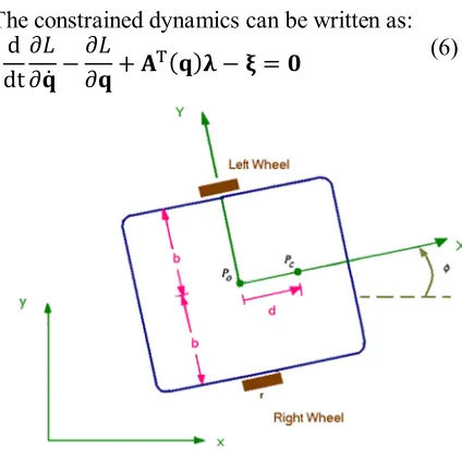
The governing equations of the system motion, mobile robot, will be derived in this section. The schematic of the system is shown in Fig. 1. As shown in Fig. 1, this mobile robot has two driving wheels, on an axis passing through the vehicle geometrical center. The shown robot wheels are powered by two D.C. motors and are not allowed to slip sideways. It is worth mentioning that point p0 is the geometric center

81

symmetry axis and the driving wheels axis. Additionally, p is the center of mass of the platform, having coordinates( , ); and b denotes the distance between each driving wheel and the longitudinal axis of symmetry. Besides, r is the radius of driving wheels.

To describe the system configuration, the position of a representative point on the platform, e.g.,( , ), the platform heading angle, i.e. , and angular displacement of right and left wheels, i.e. , should be specified. As a result, the vector of generalized coordinates of the system can be considered as = [ ] .It is assumed that the wheels of the robot are subjected to pure rolling condition. Consequently, the velocity of the point p which must be in the direction of the longitudinal axis of the mobile platform [21-22], that is

- ̇ sin + ̇ cos - ̇d=0 (1)

where d is the distance between p to p along with the positive x-axis. As the robot wheels do not slip along the longitudinal axis of the platform, the following constraints will be imposed on the robot kinematics [21-22]:

̇ cos + ̇ sin +b ̇=r ̇ (2)

̇ cos + ̇ sin −b ̇=r ̇ (3)

and ̇ and ̇ are the angular velocities of the left and right wheels, respectively.

Since Eqs. (1-3) cannot be analytically integrated and transformed into algebraic constraints, theses equations are nonholonomic which can be written in compact form using matrix/vector notation as:

A ( ) ̇ =0 (4)

To derive the equations of motion for the wheeled mobile robot, the Lagrange technique will be employed. To this end, the Lagrangian of the system should first be derived which can be obtained as:

L= m ̇ + ̇ + 2 m ( ̇ +

d ̇ sin ) + 2 m ( ̇ −

d ̇ cos ) + I ̇ + I ̇ +

[2m (d + b )] ̇ +

I ̇ + I ̇

(5)

where m , I are the mass and the mass moment of inertia of the platform, respectively. Also, m and I are the mass and mass moment of inertia of the wheels, respectively.

The constrained dynamics can be written as: d

dt ∂ ∂ ̇ −

∂

∂ + ( ) − =

(6)

Fig. 1. The schematic view of the robot, containing some of the key geometrical parameters.

where is the Lagrange multiplier vector which corresponds to the constraint forces, and represents the generalized forces. Expressing Eq. (5) in terms of the generalized coordinates and substituting the result into Eq. (6), the system equations of motion are obtained in the following form:

M( ) ̈ +V(q, ̇)= E(q) - ( ) (7)

82

v(t) = [ ̇ ̇ ] (8)

̇ = ( ). (t) (9)

where matrix S(q) contains the base vector of the null space of A. For the system at hand S(q) was chosen as

S( ) =

⎣ ⎢ ⎢ ⎢

⎡ c ∗ (b ∗ Cos − d ∗ Sin ) c ∗ (b ∗ Cos + d ∗ Sin ) c ∗ (b ∗ Sin + d ∗ Cos ) c ∗ (b ∗ Sin − d ∗ Cos )

−

1 0

0 1 ⎦

⎥ ⎥ ⎥ ⎤

where = . The governing equations of the system motion in the state space form can be written as [21, 22]:

̇= . + _{( . . ) .} (10)

where = [ ̇ ̇ ] ,

=( ) (− ̇ − ).

3. Validation of the derived system kinematics/dynamics

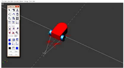
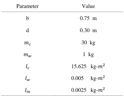
After dynamical modeling of the system in MATLAB software, in order to verify the developed dynamics equations of the wheeled mobile robot, the ADAMS multi-body simulation software is used, see Fig. 2. Toward this goal, the same actuating wheel torques are applied to both MATLAB and ADAMS models and the obtained results of these models are compared. Figure 3 shows one of these verification results which demonstrates close agreement as well as the soundness of the both models. It is worth mentioning that these results can be produced considering the values for geometrical/dynamical parameters of the mobile robot mentioned in Table 1.

It is pointed out that the obtained dynamics can be verified using ADAMS software in two ways. In the first approach (direct verification), the nonholonomic constraints, i.e. Eqs. (1-3), are imposed to the model directly. Indeed, the model in ADAMS is actuated using wheels torques while its motion is subject to various kinematic constraints.

Fig. 2. The model of the robot in ADAMS multi-body simulation software.

Fig. 3. Comparison of the response of the developed dynamics equations in MATLAB software and the model of the robot in ADAMS multi-body simulation software.

In the second approach (indirect method), no constraint is directly imposed on the robot motion. But instead, the contact model is considered and the friction between the wheel and the ground is increased such that the wheel skidding and slipping can be avoided. In this study, both approaches are adopted. The results shown in Fig. 3 are obtained based on the indirect technique and arbitrary actuating wheel torques. Notice that for this case, three kinematic constraints are considered. These constraints denote the nonholonomic Eqs. (1-3).

In Figs. 4 and 5, the results of indirect verification, at the kinematics level, are depicted. In fact, in this case, the wheels angular velocities are considered as inputs of the system. The results of ADAMS and those of the derived equations of motion are shown in Figs. 4 and 5

for = = 5 ⁄ and =

2 ⁄ , = 5 ⁄ , respectively. As seen, the obtained results are sufficiently close. In Fig. 6 the results of indirect verification, at the level

-10 -5 0 5 10

-10 -5 0 5 10

x (m)

y

(

m

)

Path generated in Adams

83

of dynamics, are demonstrated. For this case,𝜏𝑙 = 𝜏𝑟 = 0.5 𝑁. 𝑚. Again, the obtained

results reveal the soundness of the obtained motion equations. For indirect verification, where the friction is modeled, the following specifications are considered in ADAMS. The sample time is 0.001 sec. The type of friction model is Columb, whose static and dynamic coefficients are set as 0.9 and 0.8, respectively based on the recommendations given by J. Giesbers [23]. Also, the option for Normal Force in ADAMS is considered as Impact. Besides, Stiffness, Force Exponent, Damping, and Penetration Depth are considered as 1𝑒8, 2.2, 1𝑒4, and 1𝑒 − 4, respectively.

4. Formation control via leader-follower approach

In order to formation control of a group of wheeled robot, a real robot and a virtual follower robot are considered which indicate the real and desired positions of the follower, respectively.

Fig. 4. Verification at the level of kinematics

considering contact model for 𝜔𝑙= 𝜔𝑟= 5 𝑟𝑎𝑑 𝑠⁄ .

Fig. 5. Verification at the level of kinematics

considering contact model for 𝜔𝑙= 2 𝑟𝑎𝑑 𝑠⁄ , 𝜔𝑟=

5 𝑟𝑎𝑑 𝑠⁄

Fig. 6. Verification at the level of dynamics

considering contact model for 𝜏𝑙= 𝜏𝑟= 0.5 𝑁. 𝑚.

Table 1. The physical parameters of the considered wheeled platform.

Parameter Value

b 0.75 m

d 0.30 m

𝑚𝑐 30 kg

𝑚𝑤 1 kg

𝐼𝑐 15.625 kg-𝑚2

𝐼𝑤 0.005 kg-𝑚2

𝐼𝑚 0.0025 kg-𝑚2

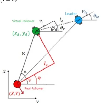
In Fig. 7, 𝑣𝑙𝑒 and 𝜃𝑙𝑒 represent the linear velocity

of the leader and the angle between 𝑣𝑙𝑒 and

horizontal direction, respectively. Besides, 𝑙e is

the distance of the real follower from the virtual one along the longitudinal axis of the real follower robot. In this study, in order to describe the position of each follower relative to the leader, the distance-angle method is adopted. When the leader and follower robots have an arbitrary arrangement relative to each other, the follower can measure its distance 𝐾 from the virtual follower and also the angle α. These variables can be derived as below:

𝐾 = √(𝑥𝑑− 𝑥)2+ (𝑦𝑑− 𝑦)2 (11)

𝛼 =atan2((𝑥d− 𝑥), (𝑦d− 𝑦)) (12)

𝑙e=(𝑥d-x)cosφ +(𝑦d-y)sinφ (13)

1 2 3 4 5

-2 -1.5 -1 -0.5 0 0.5 1 1.5 2

x(m)

y(

m

)

Path generated in Adams

Path generated by equations of motion

-2 -1 0 1

0 0.5 1 1.5 2 2.5 3 3.5

x(m)

y(

m

)

Path generated in Adams

Path generated by equations of motion

0 5 10 15

-6 -4 -2 0 2 4 6

x(m)

y(

m

)

Path generated in Adams

84

where atan2(y, x) denotes the two-argument arc tangent function. In order to control the robots formation, the above three variables (Eqs. (11- 13)) are required, as will be described in the next section. It can easily be observed that the desired robots configuration is formed when the following conditions are satisfied.

= 0 =

Fig. 7. Geometry of the relative configuration of the leader-follower robots.

4. 1. Formation control via fuzzy logic

For the problem at hand, the main question is how to compute the appropriate heading angle of the real follower robot. Should this angle be equal to α, θr, or something between α and θr? The answer is that the proper heading angle is different in various situations and it depends on the system overall configuration [12]. In this section, a proper heading angle of motion for the real follower, which is named , is determined. This angle is found via a two-stage of a fuzzy logic planner [12]. Two different cases can be considered in the first stage.

1. The real follower is far from the virtual follower. In this case, the Eq. (14) is used to calculate the proper heading angle of motion.

= . + (1 − ). (14)

where is a varying coefficient between zero and one which is obtained using the fuzzy

logic rules under linguistic variables of Table 2, and also using the fuzzy sets as shown in Figs. 8 and 9.

2. The real follower is close to the virtual follower. In order to obtain the proper heading angle of the motion, the Eq. (15) is used.

= (15)

In the second stage, the proper angle of motion for the real follower is developed as:

= (1 − ). + . (16)

where is a varying coefficient between zero and one and obtained by the logical fuzzy rules under linguistic variables of Table 3 and using the associated fuzzy sets for these rules, as shown in Fig. 10 and Fig. 11. It is noteworthy that all fuzzy planners are Sugeno type inference system.

Table 2. The rules set for generating .

Zero Small Large

Small Medium Large

Table 3. The rules set for generating .

K ZE PS PM PL PVL

Co one one PM PS PVS

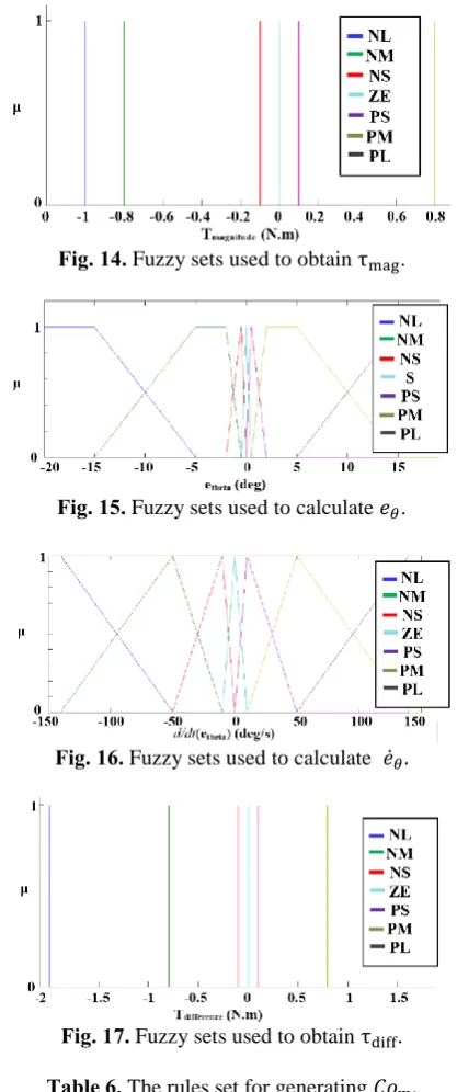
Fig. 8. Fuzzy sets used to calculate .

85

In order to control the real follower, the actuating torques applied to the right and left wheels, i.e. τl and τr, should be determined. To this end, the

torque magnitude, τmagnitude, and the torque

difference, τdifference , should be obtained.

Hence, firstly τmagnitude should be calculated

based on the distance between the real follower and the virtual one along the longitudinal axis of the real follower robot and its time derivative, i.e. 𝑙𝑒 and 𝑙̇𝑒, respectively. The considered fuzzy

logic rules under linguistic variables of Table 4, and associated fuzzy sets of these rules are shown in Figs. 12-14. After that, τdifference is

computed using eθ which can be calculated from

Eq. (17).

𝑒𝜃 = 𝜑𝑚𝑑− 𝜑 (17)

Fig. 10. Fuzzy sets used to calculate 𝐾.

Fig. 11. Fuzzy sets used to calculate 𝐶𝑜𝑘.

Fig. 12. Fuzzy sets used to calculate 𝑙e.

Table 4. The rules set for generating torque magnitude.

𝑙𝑒̇

PL P M PS ZE NS N M NL 𝑙𝑒 PL PL P M P M P M P M PS NL PL PL PL PL PL P M PS N M PL P M P M PS ZE NS N M NS N M NS ZE ZE ZE PS P M ZE NL N M N M NS ZE PS P M PS NL NL NL NL NL NL NS P M NL NL N M N M N M N M NS PL

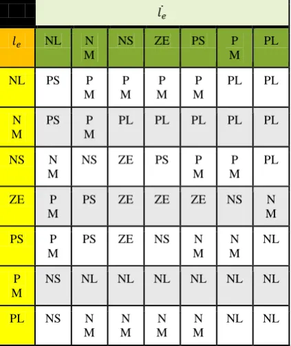
Table 5. The rules set for generating torque difference.

𝑒̇𝜃 PL PM PS ZE NS NM NL 𝑒𝜃 ZE NS NM NM NL NL NL NL PS ZE NS NM NL NL NL NM PM PS ZE NS NM NL NL NS PL PM PS ZE NS NM NL ZE PL PL PM PS ZE NS NM PS PL PL PL PM PS ZE NS PM PL PL PL PL PM PS ZE PL

86

Fuzzy rules with linguistic variables of Table 5 are used to derive τdifference. The associated

fuzzy sets, are shown in Figs. 15-17. After obtaining the torque magnitude and the torque difference, τl and τr can be found based on the

following equations:

τl+ τr= τmagnitude (18)

τl− τr= τdifference (19)

It should be noted that in Tables 3, 4, 5 and 6, ZE, V, P, N, S, M, and L stand for Zero, Very, Positive, Negative, Small, Medium, and Large quantities, respectively.

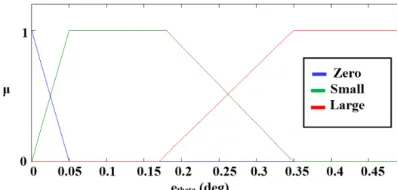
5. Modifier segment

Since τmagis generated based on the real

distance of the robot from the virtual follower; therefore, it is required to modify this command to achieve better performance of the controller. Consider the case in which the robot and the virtual follower distance is significant and at the same time, the difference between the actual heading angle and, the desired one is considerable as well. In such a case, increasing the τmagcauses increasing the robot distance

from the virtual follower. Therefore, initially when the robot starts its motion, it is more suitable that the controller provides the appropriate heading angle for the robot. Toward this aim, some sort of modifier is required to adjust the output of the τmagusing an appropriate

coefficient, i.e. 𝐶𝑜𝑚 . This coefficient lies between zero and one and is multiplied by the output of the τmag. The inputs of the modifier

include the distance 𝐾 of the robot from the virtual follower and the absolute value of the difference of the robot actual heading angle and the appropriate one, i.e. |eθ|. The considered

rules for the modifier segment are as given in Table 6 and the associated fuzzy sets shown in Figs. 18-20.

Fig. 14. Fuzzy sets used to obtain τmag.

Fig. 15. Fuzzy sets used to calculate 𝑒𝜃.

Fig. 16. Fuzzy sets used to calculate 𝑒̇𝜃.

Fig. 17. Fuzzy sets used to obtain τdiff.

Table 6. The rules set for generating 𝐶𝑜𝑚.

K

Large small

zero |𝑒Ө|

one one

one Zero

PL PM

PVS Small

PS PVS

87

segment.

Fig. 19. Fuzzy sets used to obtain of the modifier segment.

Fig. 20. Fuzzy sets used to obtain .

6. Simulation results

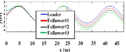
The effectiveness of the proposed methodology is examined for various scenarios. Some of the achieved results are reported and discussed here. For instance, the desired reference trajectory of the leader robot is considered as a circular path. In this case study, the groups are in column configuration as shown in Fig. 21. The responses of three follower robots in a column formation for a circular path are shown in Fig. 22. In addition, Fig. 23, demonstrates the distance of each robot from its desired position. As it can be observed, the error reduces and the robots are finally settled down to their desired positions. It is noteworthy that all robots are randomly positioned at the start time, and therefore at this moment the real distances of the robots from their desired positions are obviously significant.

In Figs. 24 and 25, the performance of the suggested methodology is examined for a more intricate motion. The response of the system against disturbance can be seen in Fig. 26. One of the important issues in the formation control is the formation switching which means changing the current formation to another one. Fig. 27 shows that the robots change their line formation to a column one after 20 seconds from the beginning of the maneuver.

Fig. 21. Desired column formation of the robot group.

88

Fig. 22. Circular path of the leader robot and the path negotiated by the followers.

Fig. 25. Path of the leader robot and path negotiated by the followers.

Fig. 23. Distance between the real position of each robot and its desired one

Fig. 26. Paths of the leader and followers while the system is subject to a disturbance.

Fig. 24. path of the leader robot and path negotiated by the followers.

Fig.27. A maneuver in which the line formation converts into a column one.

-10 0 10 20 30 40 50 60 70 80

-1 -0.5 0 0.5 1 1.5 2 2.5

89

with noisy data received from the leader robot .

Fig. 29. Ramp path negotiated by the follower robot with noisy data received from the leader robot.

Fig. 30. Comparing the response of the kinematical controller proposed by Amoozgar et al. [12] and the suggested controller of this study for a circular path.

Fig. 31. The control effort comparison for the kinematical controller proposed by Amoozgar et al.

[12] and the suggested controller of this study.

6. Conclusions

In this paper, a leader-follower based formation control of nonholonomic wheeled mobile robots has been studied via fuzzy logic and system dynamics. To this end, the dynamics of the system obtained and simulated in MATLAB software and then verified via ADAMS multi-body simulation software. Some fuzzy logic based controllers were then developed to adjust the wheels actuating torques. It was shown that the suggested dynamical controller is able to generate and keep the desired formation. Additionally, it was proved that it can handle formation change and also copes with the noisy data received from the leader robot. Finally, the performance of the suggested dynamical controller of this paper was compared against that of the kinematical controller previously presented by Amoozgar et al. [12]. The obtained computer simulations revealed the success of the suggested controller in terms of tracking and controlling effort as compared with those proposed by Amoozgar et al. [12].

References

[1] D. B. Nguyen and K. D. Do, “Formation control of mobile robots,” International Journal of Computers, Communications &Control, Vol. I, No. 3, pp. 41-59, (2006).

[2] N. H. Li and H. H. Liu, “Formation UAV flight control using virtual structure and motion synchronization,” In Proceedings of the American Control Conference, pp. 1782-1787, June 2008.

[3] G. H. Elkaim and R. J. Kelbley, “A lightweight formation control methodology,” Proceedings of the IEEE Aerospace Conference, California, No. 1096, (2006).

90

[5] J. Shao, L. Wang and G. Xie, “Flexible formation control for obstacle avoidance based on numerical flow field,” Proceedings of IEEE Int. Conf. on Decision and Control, San Diego, pp. 5986- 5991, (2006).

[6] A. Abbaspour, S. A. A. Moosavian and K. Alipour, “Formation control and obstacle avoidance of cooperative wheeled mobile robots,” International Journal of Robotics and Automation, Vol. 30, No. 5, pp. 418-428, (2015).

[7] A. Abbaspour, K. Alipour, H. Z. Jafar and S. A. A. Moosavian, “Optimal formation and control of cooperative wheeled mobile robots,” Comptes Rendus Mecanique, Vol. 343, No. 5, pp. 307-321, (2015).

[8] T. Balch , “Social potentials for scalable multi-robot formations,” In proceedings of IEEE International Conference on Robotics and Automation, San Fransisco, CA, p.p. 73-80, (2000).

[9] H. Hashimoto, “Cooperative movement of human and swarm robot maintaining stability of swarm,” Proceedings of the 17th IEEE International Symposium on Robot and Human Interactive Communication, Munich, pp. 1582-1587, August (2008).

[10] T. Balch and R. C. Arkins, “Motor schema based formation control for multi agent robot team,” In Proceedings of the International Conference of Multi-Agent Systems, San Francisco, CA, pp. 10-16, (1995).

[11] F. E. Scheider and D. Wildermuth, “A potential field based approach to multi robots formation navigation,” In Proceedings of the IEEE International Conference on Robotics Intelligent System and Signal Processing, china, pp. 608-685,October (2003).

[12] M. H. Amoozgar, K. Alipour and S. H. Sadati, “Position control of multiple wheeled mobile robots using fuzzy logic,” Journal of Industrial Robot, Vol. 38, No. 3, pp. 269-281, (2011).

[13] P. Song, “A coordination framework for weakly centralized mobile robot teams,”

IEEE International Conference of Information and Automation (ICIA), Harbin, pp.77-83, June (2010).

[14] M. Asgari, M. Jahed motlagh and K. Alipour, “Leader-follower flexible formation control of wheeled mobile robots based on an integrated bio-inspired neurodynamics approach and backstepping scheme,” Modares Mechanical Engineering, Vol. 16, No. 4, pp. 88-98, (2016).

[15] H. Mehrjerdi, “Hierarchical fuzzy cooperative control and path following for a team of mobile robots,” Mechatronics, Vol. 16, No. 5, pp. 907-917, (2011). [16] X. Li, “Robot formation control in

leader-follower motion using direct Lyapunov method,” International Journal of Intelligent Control and System, Vol. 10, No. 3, September (2005).

[17] A. S. Brandao and R. Carellit, “Decentralized control of leader-follower formations of mobile robots with obstacle avoidance,” In Proceedings of the IEEE International Conference on Mechatronics,

Spain, pp. 1-6, April (2009).

[18] M. Ghiasvand and K. Alipour, “Formation control of wheeled mobile robots based on fuzzy logic and system dynamics,” Proceedings of 13th Iranian Conference on In Fuzzy Systems (IFSC), pp. 1-6, (2013).

[19] Y. Yang, and Y. Yan, “Attitude regulation for unmanned quadrotors using adaptive fuzzy gain-scheduling sliding mode control,” Aerospace Science and Technology, Vol. 54, pp. 208-217, (2016). [20] J. J. Craig, “Introduction to robotics: mechanics and control,”3rd _{ed., Upper} Saddle River: Pearson Prentice Hall, (2005).

[21] N. Sarkar, X. Yun and V. Kumar “Control of mechanical systems with rolling constraints application to dynamic control of mobile robots,” The International Journal of Robotics Research, Vol. 13, No.1, pp. 55-69, (1994).

91

IEEE Int. Conf. on Intelligent Robots and Systems, Japan, (2000).

[23] J. Giesbers, “Contact mechanics in

ADAMS: A technical evaluation of the contact models in multibody dynamics software MSC Adams,” Bachelor Thesis, University of Twente, Netherlands, (2012).

How to cite this paper:

K. Alipour, M. Ghiasvandand B. Tarvirdizadeh, “Dynamical formation control of wheeled mobile robots based on fuzzy logic”, Journal of Computational and Applied Research in Mechanical Engineering, Vol. 6. No. 2, pp. 79-91

DOI: 10.22061/jcarme.2017.600