SOLVING A NONLINEAR INVERSE PROBLEM OF IDENTIFYING AN UNKNOWN SOURCE TERM IN A REACTION-DIFFUSION
EQUATION BY ADOMIAN DECOMPOSITION METHOD
REZA POURGHOLI1, AKRAM SAEEDI2,§
Abstract. We consider the inverse problem of finding the nonlinear source for nonlin-ear Reaction-Diffusion equation whenever the initial and boundary condition are given. We investigate the numerical solution of this problem by using Adomian Decomposition Method (ADM). The approach of the proposed method is to approximate unknown co-efficients by a nonlinear function whose coco-efficients are determined from the solution of minimization problem based on the overspecified data. Further, the Tikhonov regular-ization method is applied to deal with noisy input data and obtain a stable approximate solution. This method is tested for two examples. The results obtained show that the method is efficient and accurate. This study showed also, the speed of the convergent of ADM.
Keywords: Inverse problem; Adomian Decomposition Method (ADM); Convergence; Overspecified data; Least Square; Tikhonov Regularization Method.
AMS Subject Classification: 65M32, 35K05.
1. Introduction
The Adomian Decomposition method was called after its creator: Gorge Adomian [1], [2], [3], [13]. The method is useful for solving a variety of problems. A review of the application of the Adomian decomposition method for solving differential and integral equations was discussed in [2, 3]. It was also used for solving the linear and nonlinear heat transfer equation in [25], whereas its use for solving the wave equation was tested in [14]. In [15] the ADM was utilized for solving the inverse problems of differential equations. The method may also be employed in mathematical models describing different technical problems as discussed in [8]. The proof of the convergence for the ADM was discussed by charrault [9].
Recovery of missing parameters in partial differential equations from overspecified data plays an important role in inverse problems arising in engineering and physics. These problems are widely encountered in the modelling of interesting phenomena, e.g. heat conduction and hydrology. Another challenge of mathematical modelling is to determine
1 School of Mathematics and Computer Sciences, Damghan University, P.O.Box 36715-364, Damghan,
Iran.
e-mail: [email protected];
2
School of Mathematics and Computer Sciences, Damghan University, P.O.Box 36715-364, Damghan, Iran.
e-mail: [email protected];
§ Manuscript received: November 04, 2015; Accepted: April 05, 2016.
TWMS Journal of Applied and Engineering Mathematics, Vol.6, No.1; c⃝I¸sık University, Department of Mathematics, 2016; all rights reserved.
what additional information is necessary and/or sufficient to ensure the (unique) solvability of an unknown physical parameter of a given process. a variety of techniques for solving inverse problems have been proposed [22]- [24] Inverse source problem arises from many physical and engineering problems. Inverse source problem is known to be ill-posed in the sense that a small change in the given data may result in a dramatic change in the solution. For inverse source identification problem, there have been a lot of research results, e.g. the existence and uniqueness of the solution, [7] the conditional stability and data compatibility of the solution, [18] numerical algorithms for the identification problem. [11] Due to the ill-posedness of the problem, numerical computation is difficult. In order to obtain a stable numerical solution for this kind of ill-posed problem, some special methods are required such as Tikhonov regularization [26], iterative regularization [4], mollification [17], BFM (Base Function Method) [23], SFDM (Semi Finite Difference Method) [16] and the FSM (Function Specification Method) [5].
In this present paper we solve the problem of structural identification of an unknown source term in a class of Reaction-Diffusion equation. This equation is used to model a wide range of phenomena in physics, engineering, chemistry and biology [19]. This problem is described by the following inverse problem: Find u = u(x, t) and F = F(u) which satisfy
ut(x, t) = (A(u)ux)x+F(u), (x, t)∈QT = (0,1)×(0, T), (1.1)
u(x,0) =f(x), x∈(0,1), (1.2)
u(0, t) =p(t), t∈(0, T), (1.3)
u(1, t) =q(t), t∈(0, T). (1.4)
Subject to the overspecification
u(α, β) =k, α∈(0,1), β∈(0, T), (1.5)
Where f(x), p(t), q(t) and k are known function and A(u), is arbitrary smooth func-tion. In this context of heat conduction and diffusion when u represent temperature and concentration, the unknown function F(u) is interpreted as a heat and material source, respectively, while in a chemical or biochemical applicationF may be interpreted as a re-action term. Although the results in this paper apply to each of these interpretations, the unknown functionF(u) will be referred to here as a source term. The approach to solve this problem referred to in the literature as a method of output least squares in to assume that the unknown function is a specific functional form depending on some parameters and then seek to determine optimal parameter values so as to minimize an error functional based on the overspecified data.
The organization of this paper is as the following: we give a brief analysis of the method in section 2. Moreover, we compare the numerical results with the exact solutions and those were obtained by the ADM in section 3 and section 4 consists of a brief conclusions.
2. Analysis of the method
In the section we are considering the following inverse parabolic problems
ut= (A(u)ux)x+F(u), (x, t)∈QT = (0,1)×(0, T), (2.1a)
u(x,0) =f(x), x∈(0,1), (2.1b)
u(0, t) =p(t), t∈(0, T), (2.1c)
Wheref(x),p(t),q(t) are given functions, the indicestandxdenote differentiating with respect to these variables. A(u) is the arbitrary function, it is concentration dependent conductivity. Such problem arise in plasma and solid state physics and polymer sciences. Let us consider the linear and nonlinear operatorsL, N respectively, defined by
L(u) = ∂u ∂t,
N(u) = ∂
∂x(A(u)ux) +F(u) =
∂((A(u))
∂x ux+A(u) ∂2u
∂x2 +F(u), Then the equation (2.1a) can be written
L(u) =N(u),
The operatorL is invertible and
L−1(.) =
∫ t
0 . dt,
if we operate L−1 in the right hand side of (2.1a) and use the initial condition u(x,0) = f(x), we have
u(x, t) =f(x) +L−1(N(u(x, t)), Application to (2.1a) gives
u(x, t) =f(x) +
∫ t
0
((A(u)ux)x+F(u))dt, (2.2)
Remark 2.1. In this work the polynomial form proposed for the unknown F(u) before performing the calculation, thereforeF(u) is approximated as
F(u) =a0+a1u+a2u2+...+amum,
where{a0, a1, ..., am}are constants which remain to be determined by least squares method.
Adomians method consists in calculating the solution u of (2.2) in a series form
u=
∞ ∑
n=0
un, (2.3)
And the nonlinear term becomes
N(u) =
∞ ∑
n=0
An, (2.4)
WhereAn called Adomian polynomials [9], has been introduced by the adomian himself by the formula
An(u0, u1, ..., un) = 1 n!
dn dλn[N(
n
∑
i=0
λiui)]λ=0, n= 0,1,2, ...,
Putting equation (2.3) and (2.4) into (2.2) gives
∞ ∑
n=0
un=f(x) +
∫ t
0
(A(u)ux)x+F(u)dt,
Each term of series∑∞n=0 can be identified by the formula
{
u0(x, t) =f(x),
And theAn are determined by using the relationship
A0=a0+a1u0+a2u20+...+amum0 +A′(u0)2(u0x)2+A(u0)u0xx,
A1= 2A′(u0)u0xu1x+u1(a1+2a2u0+...+mamum0−1+A′′(u0)(u0x)2+A′(u0)u0xx)+A(u0)u1xx, A2=
1
2(2u2(a1+ 2a2u0+...+mamu m−1
0 +A′′(u0)(u0x)2+A′(u0)u0xx) +u12(2a2+...+m(m−1)amu0m−2+A(3)(u0)(u0x)2+A′′(u0)u0xx) +2u1(2A′′(u0)u0xu1x+A′(u0)u1xx) + 2(A′(u0)((u1x)2+ 2u0xu2x) +A(u0)u2xx))
.. .
In practice, all the terms of the series ∑∞n=0un cannot be determined, and we use an approximation of the solutionu from the new series
ϕn= n−1
∑
i=0
ui, with lim
n→∞ϕn=u.
2.1. least-squares minimization technique. The estimated confiscations aΥ, Υ = 0,1, ..., mcan be determined by using least squares method when the sum of the squares of the deviation between the calculatedu(α, β), u(0, β), u(1, β) by ADM and the measured k, p(β), q(β) of (1.5) and (1.3) and (1.4) at α ∈ (0,1), β ∈ (0, T) is less than a small number. The error in the estimatesE(a0, ..., am) can be expressed as
E(a0, ..., am) = (u(α, β)−k)2+ (u(0, β)−p(β))2+ (u(1, β)−q(β))2,
which is to be minimized. To obtain the minimum value of E(a0, ..., am) with respect toa0, ..., am, differentiation ofE(a0, ..., am), with respect to a0, ..., am, will be performed. Thus the system corresponding to the value ofa0, ..., am can be solved, but whenu(α, β) affected by measurement errors, the estimate ofa0, ..., am will be unstable so that we used the Tikhonov regularization method for controlling this measurement errors ( [10], [12] ).
3. Applications and Results
In this section, we are going to study numerically the inverse problems (1.1)-(1.4) with the unknown source. The main aim here is to show the applicability of the present method, described in Section 2, for solving the inverse problems (1.1)-(1.4). The inverse problems are ill-posed and therefore it is necessary to investigate the stability of the present method by giving a test problem.
Remark 3.1. In an inverse problem there are two sources of error in the estimation. The first source is the unavoidable bias deviation (or deterministic error). The second source of error is the variance due to the amplification of measurement errors (stochastic error). The global effect of deterministic and stochastic errors is considered in the mean squared error or total error, [6].
Therefore, we compute total error S by using following formulae
S =
[ 1
N −1 N
∑
i=1
(uExact(xj, ti)−uADM(xj, ti))2
]1 2
, ∀j∈ {1,2, ...,}, (3.1)
Example 1. In this example we determine u=u(x, t) andF(u) satisfying
ut= (au exp(au)ux)x+F(u), 0≤x≤1, 0≤t≤T. (3.2)
with given data
u(x,0) = 1
δlog(C1x+C2), 0≤x≤1, C1, C2 ∈R,
u(0, t) = 1 δlog((
aC12
δ +bδ)t+C2), 0≤t≤T,
u(1, t) = 1
δlog(C1+ ( aC12
δ +bδ)t+C2), 0≤t≤T.
The exact solution of this problem is
u(x, t) = 1
δlog(C1x+ ( aC12
δ +bδ)t+C2),0≤x≤1, 0≤t≤T, C1, C2 ∈R,
F(u(x, t)) =b exp(−δ u).
By using ADM and Least square we estimate a0, a1, a2 for F(u) =a0+a1u+a2u2, we have
a0 = 3.6008997282536794343512732204667,
a1= 0.020729696230948750214061070156708,
a2 = 0.000032732678806070674669042788405756,
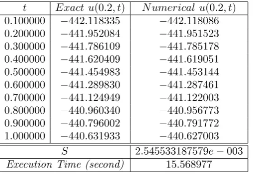
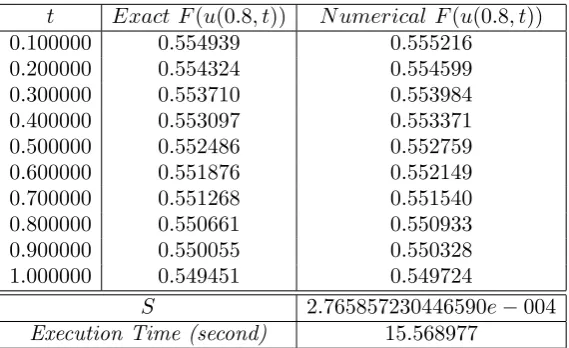
The results obtained foru(0.2, t)andF(u(0.8, t))withT = 1with noisy data are presented in Table 1, 2 and Figure 1, 2.
t Exact u(0.2, t) N umerical u(0.2, t) 0.100000 −442.118335 −442.118086 0.200000 −441.952084 −441.951523 0.300000 −441.786109 −441.785178 0.400000 −441.620409 −441.619051 0.500000 −441.454983 −441.453144 0.600000 −441.289830 −441.287461 0.700000 −441.124949 −441.122003 0.800000 −440.960340 −440.956773 0.900000 −440.796002 −440.791772 1.000000 −440.631933 −440.627003
S 2.545533187579e−003 Execution Time (second) 15.568977
t Exact F(u(0.8, t)) N umerical F(u(0.8, t)) 0.100000 0.554939 0.555216
0.200000 0.554324 0.554599 0.300000 0.553710 0.553984 0.400000 0.553097 0.553371 0.500000 0.552486 0.552759 0.600000 0.551876 0.552149 0.700000 0.551268 0.551540 0.800000 0.550661 0.550933 0.900000 0.550055 0.550328 1.000000 0.549451 0.549724
S 2.765857230446590e−004 Execution Time (second) 15.568977
0 0.1 0.2 0.3 0.4 0.5 0.6 0.7 0.8 0.9 1 −442.4
−442.2 −442 −441.8 −441.6 −441.4 −441.2 −441 −440.8 −440.6 −440.4
t
u(0.2,t)
Plot of variation u(0.2,t)
u(0.2,t) ADM u(0.2,t) Exact
0 0.2
0.4 0.6
0.8 1
0 0.2 0.4 0.6 0.8 1 −480 −460 −440 −420 −400 −380
x Plot of variation u(x,t)
t
u(x,t)
u(x,t) Surface u(x,t) ADM
Figure 1. The comparison between the exact and numerical results foru(x, t) of the problem (3.3) with the noisy data by using ADM method when
0 0.1 0.2 0.3 0.4 0.5 0.6 0.7 0.8 0.9 1 0.549
0.55 0.551 0.552 0.553 0.554 0.555 0.556 0.557
t
F(u(0.8,t))
Plot of variation F(u(0.8,t))
F(u(0.8,t)) ADM F(u(0.8,t)) Exact
0 0.2
0.4 0.6
0.8 1
0 0.5 1 0.4 0.5 0.6 0.7 0.8 0.9 1
x Plot of variation F(u(x,t))
t
F(u(x,t))
F(u(x,t)) Surface F(u(x,t)) ADM
Figure 2. The comparison between the exact and numerical results forF(u(x, t)) of the problem (3.3) with the noisy data by using ADM method when
C1=C2 =δ=a=b= 0.01 andα = 0.5, β= 0.5.
Example 2. In this example we determine u=u(x, t) andF(u) satisfying
ut= ((1−u)ux)x+F(u), 0≤x≤1, 0≤t≤T. (3.3)
with given data
u(x,0) = 1
3(2 +sinx), 0≤x≤1,
u(0, t) =1 3[
exp(−t)[3exp(2t) + 1]
exp(t) +exp(−t) ], 0≤t≤T,
u(1, t) = 1 3[
exp(−t)[3exp(2t) + 1 + 2sin1]
The exact solution of this problem is
u(x, t) = 1 3[
exp(−t)[3exp(2t) + 1 + 2sinx]
exp(t) +exp(−t) ], 0≤x≤1, 0≤t≤T,
F(u(x, t)) = 2u−2u2.
By using ADM and Least square we estimate a0, a1, a2 for F(u) =a0+a1u+a2u2, we have
a0 =−0.029470070044676017321555201200246,
a1 = 2.0756770803450796603765945006097,
a2=−2.0470530306521417537840365521654,
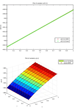
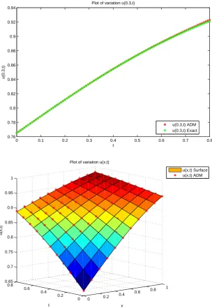
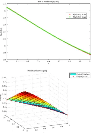
The results obtained for u(0.3, t) and F(u(0.7, t)) with T = 0.8 with noisy data are pre-sented in Table 3, 4 and Figure 3, 4.
t Exact u(0.3, t) N umerical u(0.3, t) 0.080000 0.783920 0.783981 0.160000 0.802428 0.802536 0.240000 0.820474 0.820617 0.320000 0.837854 0.838024 0.400000 0.854396 0.854596 0.480000 0.869963 0.870212 0.560000 0.884460 0.884812 0.640000 0.897827 0.898406 0.720000 0.910040 0.911081 0.800000 0.921107 0.923023
S 5.834632700437494e−004 Execution Time (second) 18.366680
Table 3. approximate solution and exact solution whenα= 0.5, β = 0.1.
t Exact F(u(0.7, t)) N umerical F(u(0.7, t)) 0.080000 0.194436 0.194963
0.160000 0.179647 0.180028 0.240000 0.164891 0.165134 0.320000 0.150365 0.150480 0.400000 0.136254 0.136244 0.480000 0.122719 0.122575 0.560000 0.109892 0.109575 0.640000 0.097876 0.097285 0.720000 0.086736 0.085674 0.800000 0.076512 0.074628
S 6.321097687149357e−004 Execution Time (second) 18.366680
0 0.1 0.2 0.3 0.4 0.5 0.6 0.7 0.8 0.76
0.78 0.8 0.82 0.84 0.86 0.88 0.9 0.92 0.94
t
u(0.3,t)
Plot of variation u(0.3,t)
u(0.3,t) ADM u(0.3,t) Exact
0 0.2
0.4 0.6
0.8 1
0 0.2 0.4 0.6 0.8 0.65 0.7 0.75 0.8 0.85 0.9 0.95 1
x Plot of variation u(x,t)
t
u(x,t)
u(x,t) Surface u(x,t) ADM
0 0.1 0.2 0.3 0.4 0.5 0.6 0.7 0.8 0.06
0.08 0.1 0.12 0.14 0.16 0.18 0.2 0.22
t
F(u(0.7,t))
Plot of variation F(u(0.7,t))
F(u(0.7,t)) ADM F(u(0.7,t)) Exact
0 0.2
0.4 0.6
0.8 1
0 0.2 0.4 0.6 0.8
0 0.05 0.1 0.15 0.2 0.25 0.3 0.35 0.4 0.45
x Plot of variation F(u(x,t))
t
F(u(x,t))
F(u(x,t)) Surface F(u(x,t)) ADM
Figure 4. The comparison between the exact and numerical results forF(u(x, t)) of the problem (2) with the noisy data by using ADM method whenα= 0.5, β = 0.1.
4. Conclusion
References
[1] Adomian,G., (1983), Stochastic Systems, Academic Press, New York.
[2] Adomian,G., (1988), A review of the decomposition method in applied mathematics, Journal of Math-ematical Analysis and Applications, 135, pp. 501-544.
[3] Adomian,g., (1994), Solving Frontier Problems of Physics: the Decomposition Method, Kluwer, Dor-drecht.
[4] Alifanov,O.M., (1994), Inverse Heat Transfer Problems. Springer, NewYork.
[5] Beck,J.V., Blackwell,B. and C. R. St. Clair, (1985), Inverse Heat Conduction: IllPosed Problems. Wiley-Interscience, NewYork.
[6] Cabeza,J.M.G., Garcia,J.A.M. and Rodriguez,A.C., (2005), A Sequential Algorithm of Inverse Heat Conduction Problems Using Singular Value Decomposition. International Journal of Thermal Sciences, 44, pp. 235-244.
[7] Cannon,J., (1984), One dimensional heat equation. California: Addison-Wesley Publishing Company. [8] Chang,M.H., (2005), A decomposition solution for fins with temperature dependent surface heat flux,
International Journal Heat and Mass Transfer, 48, pp. 1819-1824.
[9] Cherruault,Y., (1989), Convergence of Adomian method, Kybernetes, 18, pp. 31-38.
[10] Elden,L., (1984), A Note on the Computation of the Generalized Cross-validation Function for Ill-conditioned Least Squares Problems. BIT, 24, pp. 467-472.
[11] Farcas,A. and Lesnic,D., (2006), The boundary-element method for the determination of a heat source dependent on one variable. J. Eng. Math, 54, pp. 375-388.
[12] Golub,G.H., Heath,M. and Wahba,G., (1979), Generalized Cross-validation as a Method for Choosing a Good Ridge Parameter. Technometrics, 21, pp. 215-223.
[13] Grzymkowski,R., Hetmaniok,E. and Sota,D., (2002), Wybrane metody obliczeniowe w rachunku wari-acyjnym oraz w rwnaniach rniczkowych i cakowych, WPKJS, Gliwice.
[14] Lesnic,D., (2002), The Cauchy problem for the wave equation using the decomposition method, Ap-plied Mathematics Letters, 15, pp. 697-701.
[15] Lesnic,D. and Elliott,L., (1999), The decomposition approach to inverse heat conduction, Journal of Mathematical Analysis and Applications, 232, pp. 82-98.
[16] Molhem,H and Pourgholi,R., (2008), A numerical algorithm for solving a one-dimensional inverse heat conduction problem, Journal of Mathematics and Statistics, 4, pp. 60-63.
[17] Murio,D.A., (1993), The Mollification Method and the Numerical Solution of Ill-Posed Problems. Wiley-Interscience, NewYork.
[18] Yi,Z. and Murio,D.A., (2004), Source term identification in 1-D IHCP. Comput. Math. Appl, 47, pp. 1921-1933.
[19] Murray,J.D., (1989), Mathematical Biology. Springer, Berlin.
[20] Pourgholi,R. and Esfahani,A., (2013), An efficient numerical method for solving an inverse wave problem. IJCM. 10.
[21] Pourgholi,R., Esfahani,A., Rahimi,H and Tabasi,S.H., (2013), Solving an inverse initial-boundary-value problem by using basis function method. Computational and Applied Mathematics, 1, pp. 27-32.
[22] Pourgholi,R, Dana,H. and Tabasi,S.H., (2014), Solving an inverse heat conduction problem using ge-netic algorithm: Sequential and multi-core parallelization approach. Applied Mathematical Modelling, 38, pp. 1948-1958.
[23] Pourgholi,R. and Rostamian,M., (2010), A numerical technique for solving IHCPs using Tikhonov regularization method. Applied Mathematical Modelling, 34, pp. 2102-2110.
[24] Pourgholi,R., Rostamian,M. and Emamjome,M., (2010), A numerical method for solving a nonlinear inverse parabolic problem. Inverse Problems in Science and Engineering, 8, pp. 1151-1164.
[25] Soufyane,A. and Boulmalf,M., (2005), Solution of linear and nonlinear parabolic equations by the decomposition method, Applied Mathematics and Computation, 162, pp. 687-693.
Reza Pourgholi, for a photograph and biography, see TWMS Journal of Applied and Engineering Mathematics, Volume 2, No.2, 2012.