VULNERABILITY IN NETWORKS

(1)

V.AYTAC¸1, §

Abstract. Recently defined exponential domination number is reported as a new mea-sure to graph vulnerability. It is a methodology, emerged in graph theory, for vulner-ability analysis of networks. Also, it gives more sensitive results than other available measures. Exponential domination number has great significance both theoretically and practically for designing and optimizing networks. In this paper, it is studied how some of the graph types perform when they suffer a vertex failure. When its vertices are corrupted, the vulnerability of a graph can be calculated by the exponential domination number which gives more information about the characterization of the network. Keywords: Graph vulnerability, network design and communication, domination, expo-nential domination number, robustness, thorn graphs.

AMS Subject Classification: 05C40, 05C69, 68M10, 68R10

1. Introduction

Networks surround us. In the real world, networks with non-trivial topology have a broad variety of utilizations. These real-world utilizations can be exemplified as: The In-ternet, world trade Web, metabolic networks, electricity networks, supply chain networks, road networks, etc. With the introduction of small-world networks and complex networks’ scale-free properties in the literature, trying to understand the principles of organization of complex networks has attracted considerable interest within half a decade. Complex networks have a multidisciplinary research and application domain. Within this domain, there are also branches of different sciences such as social sciences and information as well as basic sciences. The staple topic that is used to get the measure of stability and robustness of complex networks is that of vulnerability. The total resistance of a network’s underlying graph can be defined as the vulnerability of that network. While obtaining an underlying graph of a network, main components are the nodes and the links. The links connect two nodes that mutually send information. Both the node and link vulnerability of complex networks can be examined; that is, it is possible to discuss how the network is affected by removing any combination of nodes and links from the network.

Various methods have been introduced to characterize vulnerability of networks. Assume thatG= (V(G), E(G)) is a graph which has these characteristics : non-directional, simple and connected. Generally, a network is modeled as a non-directional and simple graph.

1 _{Department of Computer Engineering, Faculty of Engineering, Ege University 35100, Izmir, Turkey.} e-mail: [email protected]; ORCID: https://orcid.org/0000-0002-0038-6180.

§ Manuscript received: May 17, 2017; accepted: October 20, 2017.

(2)

In this model, while processors are taken as vertices, connections between the processors are taken as edges. As the most powerful mathematical tool, graph theory plays an im-portant role to analyze and understand the architecture of a network. When the network requirements are stated within theoretical graph parameters, the analyzing and designing problem of networks turns into obtaining a graph G that meets some particularized re-quirements.

In the literature, several metrics have been given to determine the robustness value of nets. Moreover, to calculate the reliability of nets some parameters which belong to graph theory have been used. For instance, connectivity, toughness, integrity, domination, scat-tering [3, 13, 16]

In this study, the non-directional, finite and simple graph is within our care. Also, it does not have loops and multiple edges. Let’s take a graph G = (V(G), E(G)) by assuming V is a set of vertices and E is a set of edges. Wherein V(G) 6= ∅ and E(G) is a subset of V(G)×V(G). Let’s remember some common definitions that we will encounter and use in this study. The complement G of a graph G hasV(G) as its vertex sets, but two vertex are adjacent in G if only if they are not adjacent in G. That is, to generate the complement of a graph, one fills in all the missing edges required to form a complete graph, and removes all the edges that were previously there. The open neighborhood set of any vertex v in V(G) is formed by the vertices u ∈V(G) which are neighbors of the vertexvand this set is represented asNG(v). Besides, the closed neighborhood set of any vertex v ∈ V(G) can be obtained from by adding v to its open neighborhood set. The closed neighborhood set represented by NG[v]. The cardinality of an open neighborhood set of a vertex v gives us the degree of v and it is represented by deg(v). Consider the path with the minimum length connecting any twou1 andu2 vertices of G, the length of this path is denoted by d(u1, u2). This is indicated by d(u1, u2) =∞ if there is no path connecting u1 and u2 vertices. It is also indicated by d(u1, u2) = 0 if u1 and u2 are the same. The maximum value of the minimum paths between each pair of (u1, u2) vertices inG, is defined as diameter. It is denoted bydiam(G)[8-9].

Let S is a subset of the vertices set of G. If the elements of S are subtracted from the vertex setV(G), we get difference set. If all vertices of the set we have is connected to at least one vertex in the setS, the set we have obtained by subtracting is a dominating set. Within G’s all dominating sets, the size of the dominating set which has the minimum cardinality is named as the domination number of graphGand it is indicated byγ(G). The definition given immediately above is a rapidly growing and significant research topic that has attracted interest in the graph theory in recent years. This rapid growth can be explained by the variety of its applicability to real-world problems as well as to theory. For instance, facility location problems are modeled naturally as dominating sets in graph theory. The number of domination is foremost significant vulnerability parameters for nets. There are several domination parameters in the literature [2, 4-5, 12].

(3)

calculating the smallest quantity of origins required so that each person gets fully reliable information.

This study deals with the exponential domination number of graphs which is a new char-acteristic for graph vulnerability introduced by Dankelmann [6]. This new parameter is closely in relation with a distance of each pair of vertices. LetGas a graph andS ⊆V(G). When Gis induced by the S vertices subset, we get a subgraph of the original graph G. This subgraph is indicated byhSi. ∀u1 ∈S and∀u2 ∈V(G)−S, if there is a path between u1 and u2 vertices, d(u1, u2) = d(u2, u1) defined as the shortest path length in hV(G)−

(S− {u1})i, otherwise d(u1, u2) =∞. Letv∈V(G). The definition is

ws(v) =

_P

u∈S1/2d(u,v)−1, ifv6∈S

2, otherwise

We refer to ws(v) as the weight of S at v. If ws(v) ≥ 1, ∀v ∈ V(G) then S can be an exponential dominating set. Within all exponential dominating set of G, the size of the exponential dominating set with the smallest cardinality is named as the exponential domination number of graphGand it is indicated by γe(G). Also, minimum exponential dominating set ofG denoted byγe –set. Letu1 ∈S and u2 ∈V(G)−S,u1 exponentially dominatesu2, if 1

2d(u10u2)−1 >0[1, 6-7, 11].

The study continues as follow. Section 2 gives the theoretical background and an overview of results on the exponential domination number. Main results for the exponential domi-nation number of particular types of graphs and regular caterpillars are provided in Section 3 while giving an insight of how to evaluate the parameter and derive formula on path type networks.

2. Basic results

In this part of the study, some known basic results related to exponential domination number in the literature are given.

Theorem 2.1. [6] The exponential domination number of

(a) the path graphPn of order n≥2 is γe(Pn) =d n+ 1

4 e.

(b) the cycle graphCn of order n≥4 is γe(Cn) =

2, if n= 4

dn₄e, if n6= 4

Theorem 2.2. [6] For every graph G, γe(G) ≤γ(G), and also γe(G) = 1 if and only if γ(G) = 1.

Theorem 2.3. [1] If Gis connected graph, |V(G)|=n and there is a vertex of Gwith a degree of n−1. Then, γe(G) = 1.

Theorem 2.4. [1] If G is a connected graph, |V(G)|= n, diam (G) = 2 and there isn’t any vertex such thatdeg(v) =n−1. Then, γe(G) = 2.

Theorem 2.5. [6] If Gis a connected graph of diameter d, then γe(G) =d d+ 2

4 e.

Theorem 2.6. [6] If Gis a connected graph and |V(G)|=n thenγe(G)≤ 2

5(n+ 2).

(4)

Theorem 2.8. If the diameter of G is at least 3, then γe(G) = 2.

Proof. Assume that u and v are two vertices such thatdG(u, v) = 3. Since dG(u, v) = 3, N(u)∩N(v) =∅. Assume that S is a minimum exponential dominating set inG. Firstly, we assume thatS consists of the vertex u, that isS ={u}. Forx∈V(G)−S, two cases arise.

Case 1. Letx6∈NG(u).

In this case, u is connected to x in G. Therefore, S in G is exponentially dominates the vertexx.

Case 2. Letx∈NG(u).

In this case,d_G(u, x) = 2. The vertex u contributes 1

2 to ws(x). Thus we must add new one vertex toS. When this new vertex is added to S, at least one vertex ofS should not be connected to the vertexx inG. This requires that v, because dG(u, v) = 3. Hence, we getS= {u, v} and|S|= 2.

By Case 1 and Case 2, the exponential domination number ofGis γe(G) = 2.

In graph theory, complement graphs discussed in the previous theorem have a great importance. Because, there are lots of theoretical graph concepts which contains com-plement graph concept. Therefore, the information we obtain about the comcom-plement of a graph will allow us to make comments for other related graph concepts as well. For example, a graph without edges is the complement of a complement graph. Also, regular graphs play an important role in determining isomorphic structures due to their specific properties.

Theorem 2.9. Let G be a r–regular graph with order n. Then, γe(G) =d

2(n+ 1) 3r+ 2 e.

Proof. If u and v are vertices in G then [u, v] will denote the G’s all vertices set that lie on at least one u−v geodesic. Let S be a minimum exponentially dominating set of G. It is obvious that each vertex of G−S is exponentially dominated by at most two vertices of S. Let u ∈ S and v ∈ S, on G such that [u, v]∩S = {u, v} and u = u0, u1, . . . , ur

2, u

r

2+1, ur, ur+1, . . . , u32r+1 =v theu−vpath inG. The vertexucontributes 1

2 tows(ur2+1), sovmust contribute at least 1

2 tows(ur2+1). This implies thatd(u, v)≤4. Since∀v ∈V(G),deg(v) =r, the number of the vertices in [u, v] is at most 3r+ 2

2 . This leads ton≤(3r+ 2

2 )γe(G)−1.

To see thatγe(G) =d

2(n+ 1)

3r+ 2 e, we note that easy to construct exponential dominating

set with|S|=d2(n+ 1)

3r+ 2 e

3. The exponential domination number of some thorn networks

In this section, we give a definition of thorn network. Then, we calculate the exponential domination number of some thorn networks.

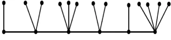
Definition 3.1. [10] Let pi be in the set Z∗={0} ∪Z+, V(G) be the vertices of graphG

(5)

with1≤i≤n and1≤j≤pi. The representation of the thorn graph of the graphG is in the formG∗ or G∗(p1, p2, . . . , pn).

P₆∗(1,2,3,2,1,4)

Figure 1. A thorn graph ofP6

Theorem 3.1. Let P_n∗ be thorn graph ofPn withpj ≥1, i∈ {1,2, . . . , n}. Thenγe(Pn∗) =

bn+ 2

2 c.

Proof. Label the vertices of Pn by u1, u2, . . . , un and let the new vertex attached to the vertex ui of the graph be uij, j ∈ {1,2, . . . , pi}. It is obvious that deg(uij) = 1 and

deg(ui) ≥ 2. Let S = {u2i+1|i ∈ {0,1, . . . ,b diam

2 c}}. Any vertex u in S dominates all adjacent vertices. Consider the verticesx ∈ (V(P_n∗)−X

u∈S

N[u]). The vertices x are the

thorns of vertices inV(Pn)−S.These vertices are at distance 2 to exactly two vertices in S. This implieswS(v) ≥1 for∀v ∈ V(Pn∗). So, the elements of S set dominate either all vertices ofV(P_n∗) or some vertices of V(P_n∗) remain undominated and then we have

γe(Pn∗)≥ |S|= 1 +b diam

2 c.

LetS∗ be a minimum exponential dominating set ofP_n∗ and S∗ contains all vertices ofS. Depending on the value ofn, two cases arise.

Case 1. Letn≡0 (mod 2).

In this case,S∗ ={u1, u2, . . . , un−1}. Then, the setS∗ contributes 1/2 to wS∗(u_nj). For

the vertexunj, ws∗(u_nj)≥1 does not satisfied. So, one vertex which is either any vertex

unj or the vertexun must be added toS∗. Then we have

γe(Pn∗)≥ |S∗|= 1 + 1 +

diam−1

2 =

diam+ 3 2 .

Case 2. Letsn≡1 (mod 2).

If S∗ contains all vertices of S and only them, all vertices of V(P_n∗) are exponentially dominated byS∗. Thus, |S∗|=|S|for this case. Hence, we get

γe(Pn∗)≥ |S

∗_|

=|S|= 1 +diam 2 =

diam+ 2 2

It is easy to say that from Case1, the set{u1, u2} is γe−set ofP2∗ and γe(P2∗) = 2. But, S={u1}forP2∗according to the definition ofS given above. S∗− {u1}isγe−setofPn∗−2. That is{u1, u2} − {u1}={u2} must be removed fromS∗. By an inductive argument, we obtain

(6)

We examine all cases usingdiam=n−1 and inductive argument. Thus, we obtain from Case1,

n−1 + 3

2 =

n+ 2

2 ≤γe(P

∗

n)≤2 +

(n−3) + 3 2 −1 =

n+ 2 2 .

Hence, we getγe(Pn∗) = n+ 2

2 . Similarly, we have from Case2,

n−1 + 2

2 =

n+ 1

2 ≤γe(P

∗

n)≤2 +

(n−3) + 2 2 −1 =

n+ 1 2

Thus, we haveγe(Pn∗) = n+ 1

2 . It is obvious that n+ 1

2 =b n+ 2

2 c and n+ 2

2 =b n+ 2

2 c. As a result, γe(P

∗

n) =b n+ 2

2 c is obtained.

Theorem 3.2. Let C_n∗ be thorn graph ofCnwithpi ≥1, i∈ {1, 2, . . . , n}. Thenγe(Cn∗) =

bn+ 1

2 c.

Proof. The proof can be made like the proof of Theorem 3.1.

Theorem 3.3. LetK_m,n∗ be thorn graph ofKm,n withm≥nandpi ≥1, i∈ {1, 2, . . . , n}. Thenγe(Km,n∗ ) is 2.

Proof. Let (K_m,n∗ ) =V1∪V2∪V10∪V20 , where V1 ={u1, u2, . . . , um},

V2 ={u1, u2, . . . , um+n},

V₁0={uij|1≤i≤m and1≤j ≤pi}. Let uij be the thorn the vertices ofV1.

V₂0 ={urs|m+ 1 ≤r ≤m+n and1 ≤s≤pr}. Let urs be the thorn the vertices of V2. The distance between the vertices of these vertices sets is as follows:

Letuij anduxy be distinct vertices in V10. d(uij, uxy) =

2, ifi=x 4, ifi6=x

This value is also some for any two distinct vertices ofV₂0.

The distance between any two vertices, one inV₁0 and the otherV₂0, is 3.

The distance between any two vertices, one in V₁0 and the other V2 or one inV20 and the otherV1 or one in V1 and the otherV1 or one inV2 and the other V2, is 2.

Let S∗ be a minimum exponential domination set K_m,n∗ . According to the distance examined above,S∗ must contain exactly two vertices ofV1 orV2. Hence,|S∗|= 2 and all vertices ofK_m,n∗ are exponentially dominated. Consequently, the exponential domination

number ofK_m,n∗ is 2.

Theorem 3.4. Let K₁∗_,n₋₁ be thorn graph of K1,n−1 with pi ≥ 1, i ∈ {1,2, . . . , n} and n≥5. Then γe(K1∗,n−1) = 4.

Proof. LetS∗be a minimum exponential domination setK₁∗_,n−1. As might be seen thatS∗ must not contain the central vertexcinK1,n−1. IfS∗consists of all vertices in (V(K1,n−1)−

{c}), all vertices inK₁∗_,n₋₁are exponentially dominated. But, in this caseS∗ must not be minimum exponential domination set. Therefore, S∗ should be consist of some vertices in (V(K1,n−1)− {c}). The distance between the thorn vertex u and the vertex v ∈

(7)

d(u, v) =

1, ifv∈N(u) 3, otherwise.

We assume that S∗ contains only one vertex v ∈ (V(K1,n−1)− {c}). We must find minimum number of vertices ofS∗ that provides

wS∗(v) =

X

u∈S∗

(1 2)

d(u,v)−1_≥₁

wherev is thorn vertex ofK₁∗_,n₋₁. Sinced(u, v) = 3,

|S∗\{u}| = 2d(u,v)−1−1 = 22−1 = 3.

Hence, |S∗|= 4. Then, all vertices in K₁∗_,n₋₁ are exponentially dominated by S∗. Consequently, the exponential domination number ofK₁∗_,n−1withn≥5 is

γe(K1∗,n−1) = 4.

Theorem 3.5. Let W₁∗_,n−1 be thorn graph of W1,n−1 with pi ≥ 1, i ∈ {1, 2, . . . , n} and n≥5. Then γe(W1∗,n−1) = 4.

Proof. The proof can be made like the proof of Theorem 3.4.

The concept of thorn graphs proposed recently by Ivan Gutman to study of chemical graphs [10]. Danail Bonchev and Douglas J Klein extended this idea to a more general concept of thorny graph. Since it represents the structural formula of aliphatic hydro-carbons and aromatic hydrohydro-carbons, this graphs’ class has great significance in spectral theory.

Calculation of exponential domination number for some thorn graph types is impor-tant. Because when more complex networks are fragmented into smaller networks, for an optimization problem, the solutions on small networks can be unified as a solution on a large network, in some circumstances.

4. Conclusion

Exponential domination can be a model for the reliability of a spreading information or a hearsay. In this model, distance exponentially reduces the dominating strategy of any vertex of a graph G, by the factor 1/2. By using exponential domination number, the vertices within a network can be identified which are more important than others and responsible for the fast communication flow. The vertices that give the number of exponential dominating of a graph are fast in distributing information over the network.

References

[1] Aytac, A. and Atay, B., (2016), On Exponential Domination of Some Graphs, Nonlinear Dynamics and Systems Theory, 16(1), pp. 12-19.

[2] Aytac, A. and Turaci, T., (2015), Vulnerability Measures of Transformation GraphGxy+, International Journal of Foundations of Computer Science, Vol. 26, issue No 6, pp. 667- 675.

[3] Haynes, T. W., Hedeniemi, S. T., Slater, P. J., (1998), Domination in graphs, Advanced Topic, Marcel Dekker, Inc, New York.

(8)

[5] Slater P.J., (1976),R-Domination in graphs, J. Assoc. Comput. Mach., 23, 446-450.

[6] Dankelmann, P., Day, D., Erwin, D., Mukwembi, S., Swart, H., (2009), Domination with exponential decay, Discrete Mathematics, 309, 5877-5883.

[7] Anderson, M., Brigham, R. C., Carrington, J. R., Vitray, R. P., Yellen J., (2009), On Exponential Domination ofCmxCn, AKCE J. Graphs. Combin., 6, No. 3, pp. 341-351.

[8] West, D. B., (2001), Introduction to Graph Theory, Prentice-Hall, NJ.

[9] Chartrand G., Lesniak, L., (1986), Graphs and Digraphs, Second Edition, Wadsworth, Monterey. [10] Gutman, I., (1998), Distance of thorny graphs, Publ. Inst. Math., (Beograd), 63(31−36), 73-74. [11] Henning, Michael A., Jager, S., Rautenbach, D., (2017), Relating domination, exponential domination,

and porous exponential domination, Discrete optimization, 23, pp:81-92.

[12] Goddard, W., Henning, M., McPillan, C., (2014), The disjunctive domination number of a graph, Quaest. Math., 37, pp. 547-561.

[13] Chv`atal, V., (1973), Tough graphs and Hamiltonian circuits, Discrete Mathematics, 5, 215-228. [14] Barefoot, C. A., Entringer, R. and Swart, H., (1987), Vulnerability in graphs–a comparative survey,

J. Combin. Math. Combin. Comput., 1 13-22.

[15] Woodall, D. R., (1973), The binding number of a graph and its Anderson number, J. Combin. Theory Ser. B, 15, 225-255.

[16] Jung, H. A., (1978), On a class of posets and the corresponding comparability graphs, Journal of Combinatorial Theory, Series B24(2), 125-133.